Learning-Based Optimal Admission Control in a Single-Server Queuing System
Abstract
We consider a long-term average profit–maximizing admission control problem in an M/M/1 queuing system with unknown service and arrival rates. With a fixed reward collected upon service completion and a cost per unit of time enforced on customers waiting in the queue, a dispatcher decides upon arrivals whether to admit the arriving customer or not based on the full history of observations of the queue length of the system. Naor [Naor P (1969) The regulation of queue size by levying tolls. Econometrica 37(1):15–24] shows that, if all the parameters of the model are known, then it is optimal to use a static threshold policy: admit if the queue length is less than a predetermined threshold and otherwise not. We propose a learning-based dispatching algorithm and characterize its regret with respect to optimal dispatch policies for the full-information model of Naor [Naor P (1969) The regulation of queue size by levying tolls. Econometrica 37(1):15–24]. We show that the algorithm achieves an O(1) regret when all optimal thresholds with full information are nonzero and achieves an regret for any specified in the case that an optimal threshold with full information is 0 (i.e., an optimal policy is to reject all arrivals), where N is the number of arrivals.
Funding: A. Cohen is partially supported by the National Science Foundation [Grant DMS-2006305]. V. Subramanian is supported in part by the NSF [Grants CCF-2008130, ECCS-2038416, CNS-1955777, and CMMI-2240981].
1. Introduction
We consider admission control for a first-in, first-out (FIFO) single-class, single-server queuing model with Poisson arrivals and exponential service times. Specifically, there is a dispatcher that decides on admitting arrivals with the goal to maximize the long-term average profit; each admitted arrival yields a positive reward R (obtained after a customer finishes service), which is balanced by a holding cost for the (homogeneous) customers waiting in the queue. The buffer capacity of this queue is infinite, and the dispatcher may decide upon arrivals to reject any customers joining the queue with the profit objective in mind. When the service and arrival rates are known, this model is studied in Naor (1969). In our investigation, we consider the situation in which the dispatcher does not have knowledge of either the arrival rate or the service rate. One potential application is the job-dispatching problem for online computing demands, especially when the computing servers are provided by a third-party cloud-computing platform: the dispatcher may negotiate the reward and cost with the customers and, thus, have information (via market research) on the arrival rate of the jobs, but because the servers are provided by a third-party platform, the dispatcher may not know the service rate. Despite prior market research, it is, however, plausible that the dispatcher doesn’t know the arrival rate accurately.
Naor (1969) studies two problems: (1) the optimal policy for the self-optimization problem in which customers are maximizing their own net (expected) profit so that a selfish Wardrop equilibrium is of interest as well as (2) the optimal policy for the social welfare–maximization problem in which a dispatcher is aiming at maximizing the long-term average profit so that a social Wardrop equilibrium is of interest. In both problems, a threshold policy is shown to be optimal: (1) in the self-optimization problem, arrivals do not join the queue if the queue length upon arrival is high enough, and (2) in the social welfare–maximization problem, the dispatcher doesn’t admit arrivals whenever a threshold level is reached. Naor (1969) shows that the threshold for the social welfare–maximization problem is not greater than the threshold for the self-optimization problem. Our investigation and the accompanying algorithm are primarily designed for the social welfare–optimization problem in which the dispatcher is interested in learning how to perform at the same level of efficiency as if knowing the actual arrival and service rate. Any learning-based algorithm necessarily needs exploration that could violate incentive-compatibility constraints (even ex ante and not only ex post) of individual utility-maximizing agents. Hence, we do not consider the self-optimization version of the problem in this manuscript.
In our analysis, we couple two queuing systems: a learning system, whose dispatcher does not know the arrival and service rate a priori, and a genie-aided system, whose dispatcher has full information of the model parameters. We refer to the corresponding algorithm and dispatcher of the two systems as the learning algorithm, learning dispatcher and genie-aided algorithm, genie-aided dispatcher, respectively. Our figure of metric at a given time t is the difference between the net expected profits of a genie-aided algorithm and the learning algorithm, that is, the expected regret.
1.1. Contributions
We propose a learning-based dispatching algorithm that achieves an O(1) regret when (genie-aided) optimal algorithms use a nonzero threshold and achieves an regret for any specified when it is optimal to use threshold 0, where N denotes the number of arrivals;1 see Remark 4 for a refinement on the achievable regret. Our learning-based algorithm consists of batches with each batch being composed of an optional forced exploration phase (phase 1) and an exploitation phase (phase 2) whose length increases with batch index. The exploration phase is omitted if there are new samples collected from the exploitation phase that just ended. Our learning algorithm uses samples collected from all the exploitation phases as well as from any exploration phases; the former is important if the exploration phase is omitted.
For the system studied in Naor (1969), not all values of the unknown model parameters result in a unique optimal static threshold policy. For some specific choices of the model parameters, there exist two optimal static thresholds, and therefore, all the policies that stochastically alternate between the two static optimal thresholds also achieve the optimal long-term average profit. As mentioned earlier, we are interested in analyzing the regret, defined to be the difference between the expected profit of the learning and genie-aided systems. When the optimal policy is unique, there is no ambiguity in the definition of the regret as there is a fixed optimal policy against which to compare. However, when there are multiple policies that are optimal, we need to specify a particular optimal policy against which we are comparing. Among the multiple optimal policies, we compare against a policy with a specific way of randomizing between the two static optimal thresholds, and then, we prove that we can achieve similar regret as when there exists a unique optimal policy, which is of order O(1) when both thresholds are positive and of order for any specified when 0 is an optimal threshold and N is the number of customers that have arrived; Remark 4 applies with nonunique thresholds too.
In our setting, we do not exclude the case in which the genie-aided dispatcher uses a static threshold zero and, hence, rejects all customers. This leads to a balancing act for the dispatcher: quickly transitioning to reject all customers if the true threshold is zero versus admitting customers infinitely often otherwise (based on the optimal threshold) and all of this when not being aware of the true optimal admission policy. With this in mind, for learning to not stall, the existence of the exploration phase is crucial when the true threshold is positive. A naive learning scheme that only uses the empirical average service time as an estimate of the unknown parameter may perform poorly: a few extremely long service times at the beginning may mislead the learning dispatcher to think that the service rate is low and, hence, result in it not accepting customers into the queue even when the genie-aided dispatcher uses a nonzero threshold; see plots in Section 6.
1.2. Related Work
On the topic of finding optimal controls vis-à-vis individual and social welfare maximization, there are many models that study generalizations of the model introduced in Naor (1969). Knudsen (1972) generalizes the model in Naor (1969) to multiple servers with a nonlinear cost for customers waiting in the system. The reward for customers served is constant, and customers arrive according to a Poisson process. The service times of the customers are exponentially distributed and are independent of the identity of the currently active server. Lippman and Stidham (1977) study a single-queue model with Poisson arrivals and nondecreasing, concave service rate with respect to the number of customers in the system. The holding cost per unit of time for each customer is constant, and the rewards for the customers entering the system are independent and identically distributed (i.i.d.) random variables with finite mean. The authors first consider the discounted net profit in the finite-horizon case (in terms of the total number of admissions and service completions) and then extend the analysis to the nondiscounted and infinite-horizon case. Johansen and Stidham (1980) study the problem of finding the optimal admission policy of a system with general service and arrival processes. In the problem’s setting, the net profit is discounted, and the authors consider the finite-horizon (in terms of the number of arriving customers) case. The rewards of the customers are i.i.d. random variables with finite mean, and the nonnegative waiting cost is a function of the number of customers in the system as well as the total number of past arrivals. All the works—Knudsen (1972), Lippman and Stidham (1977), and Johansen and Stidham (1980)—compare the optimal policy for the individual- and social welfare–maximization problems and show that the optimal policies for both optimization problems are threshold policies that depend on the rewards of customers. Moreover, they also show that the optimal threshold for the social welfare–maximization problem is no greater than the individual-maximization problem. Assuming a random arrival rate, Chen and Hasenbein (2020) show that the optimal thresholds for the social welfare–maximization problem are no larger than the individual-maximization problem when the queue length is either observable or unobservable. They also show that the optimal threshold for the revenue-maximization problem may not coincide with the social welfare–maximization problem when the queue is unobservable.
Learning unknown parameters to operate optimally in queuing systems and analyzing queuing systems with model uncertainly are both studied under various settings; see the tutorial Walton and Xu (2021) for a recent overview. Our paper focuses on regret analysis in comparison with an optimal algorithm when the parameters are known. Under this framework, there is growing literature considering different models and various types of regret. Adler et al. (2022) consider an Erlang-B blocking system with unknown arrival and service rates in which a customer is either blocked or receives service immediately. The authors propose an algorithm that observes the system upon arrivals and converges to the optimal policy that either admits all customers when there is a free server or blocks all customers. In our setting, the queue has infinite capacity; customers may wait in the queue, and the dispatcher observes the whole history of the queue length when making a decision. The reward of admitting a customer in both our paper and Adler et al. (2022) is only realized in the future as it involves knowledge of service times and (in our case also) waiting times, and the expected net profit requires knowledge of the arrival and service rates; this precludes the direct use of reinforcement learning–based methods discussed in Sutton and Barto (2018) and Bertsekas (2019). Stability is always assured in Adler et al. (2022) because the maximum system occupancy is bounded (finite number of servers with no queuing). The queuing system is stable under any optimal policy for the problem we consider. However, under an arbitrary learning dispatcher, the supremum of the queue lengths may be unbounded when the service rate is unknown. We discuss the impact of this on our analysis in Section 2.3. Krishnasamy et al. (2018a) first consider a discrete-time, single-server queuing system with multiclass customers and unknown service rates and then modify and extend their algorithms to parallel, multiserver queuing systems, again with multiclass customers. In the model, customers of class i have (per unit time) waiting cost ci when waiting in the queue and Bernoulli services with the service success probability at server j being for class i (i.e., geometrically distributed service times). They propose a rule–based algorithm that achieves constant regret compared with using the rule with the true service rates. The rule prioritizes the service of customers of type i at server j when is higher. Optimality of the rule is proved in various settings, especially in the single-server case; see Smith (1956), Shwartz and Makowski (1986), Buyukkoc et al. (1985), and (Cox and Smith 1961, chapter 3). Zhong et al. (2022) consider the problem of learning the optimal static scheduling policy in a multiclass, many-server queuing system with time-varying Poisson arrivals. Customers of type i have exponentially distributed patience with rate θi and exponentially distributed service requirements with rate μi. Unlike in Krishnasamy et al. (2018a), in which stability is not guaranteed for arbitrary scheduling policies, the impatience of the customers helps to stabilize the queue without any extra requirements on the scheduling policy. The authors compare their learn-then-schedule learning algorithm with the rule and show that their learning algorithm achieves a regret, where T is the (finite) time horizon. For a discrete-time, multiclass, parallel-server system, when compared with the algorithm that matches a queue to a server for which the success service probability is the highest among all possible matches of this queue to any other server, Krishnasamy et al. (2021) use a multiarmed bandit viewpoint and propose Q-UCB and Q-Thompson sampling algorithms that achieve queue regret as the time horizon T goes to infinity. Stahlbuhk et al. (2021) focus on a single-server, discrete-time queue and show the existence of queue length–based policies that can achieve an O(1) regret. When each server has its own queue, Choudhury et al. (2021) study the discrete-time routing problem when service rate and queue length are not known. Taking a Markov decision process (MDP) viewpoint, Agrawal and Jia (2022) consider a discrete-time, inventory-control problem in which orders to be made arrive with delay and the decision maker observes solely the sales and not the demands. Thereafter, a holding cost is collected for each unit of the good that is in storage. At each time step, the decision maker needs to make new orders and aims to minimize the total expected holding cost. The authors study the problem of learning the proper units of orders to be made at each time step when the distribution of the demand is unknown. The algorithm they propose achieves an regret (for horizon T) when compared with the best base-stock policy.
With the goal of stabilizing the queues and also minimizing penalties enforced in a discrete-time system, Neely et al. (2012) propose an algorithm that learns a set of max-weight functionals that depend on the unknown underlying distribution and make two-stage decisions (which are shown to correspond to scheduling choices in illustrated examples). The proposed algorithm stabilizes the system considered and achieves at most linear regret in the accumulated penalties when compared with the optimal controller. Considering a scheduling problem with unknown arrival and channel statistics, Krishnasamy et al. (2018b) study a wireless scheduling problem with switching costs. Under their proposed explore–exploit policy with the exploration probability going to zero slowly, together with a max-weight scheduling policy using learned statistics, the network is shown to be stable, and the algorithm achieves at most linear regret in the accumulated switching and activating cost when compared with the optimal scheduler with the knowledge of the model statistics. The error bound on the long-term average in both works can be made arbitrarily small (when compared with the optimal cost) by changing algorithm parameters. Instead of having explicit exploration, Yang et al. (2023) study a discrete-time, multiserver queuing system and propose a max-weight with discounted upper confidence bound (UCB) scheduling algorithm. Their main result shows the stability of the queuing system under the proposed algorithm.
There is a growing literature that studies online dynamic pricing in service systems using queuing models. We discuss some relevant recent work next. The authors of Chen et al. (2023) consider optimal pricing with congestion in a queue in which the unit cost depends on the service rate, the arrival rate depends on the service fee, and customers experience congestion given by the average queue length of the system. As the cost as a function of the service rate and the dependence of the arrival rate in chosen price is unknown, the authors propose a gradient-based online learning algorithm that achieves a sublinear regret when compared with the accumulated profit obtained with the optimal service rate and fee (using steady-state quantities). Also, considering an online learning version of finding a proper price among a finite set of prices, Jia et al. (2022) consider a multiserver queuing model with Poisson arrivals and exponential services in which the dependence of arrival and service rate prices chosen is unknown (with the values unknown as well but such that the load for each choice is strictly less than one). Two online batch-processing algorithms based on UCB and Thompson sampling are proposed in Jia et al. (2022). Both algorithms achieve sublinear regret (optimal up to logarithmic factors) when compared with the accumulated profit achieved by the optimal price choice.
In our work, we consider a paradigm in which there’s uncertainty in the model parameters. A different type of uncertainty, often called Knightian uncertainty, is studied in Atar et al. (2022), Cohen (2019a, b), and Cohen and Saha (2021) for multiclass queuing systems in the heavy traffic regime. In these models, the decision maker is looking for robust control for a class of models. The uncertainty is modeled by including an adversarial player who chooses a worst case scenario. Hence, the robust control problem is formulated via a stochastic game between the decision maker and the adverse player. Optimality is then characterized by studying Stackelberg equilibria.
1.3. Outline of the Paper
In Section 2, we introduce the model, propose our learning algorithm, and state our main results. In Section 3, we state some preliminary results, including the properties of the coupling introduced in Section 2. Sections 4 and 5 are devoted to the analysis of our learning algorithm and include the proof of our main results. Section 6 provides the finite-time performance of our algorithm via simulations. In Section 7, we summarize our result.
2. The Learning Problem and the Main Results
In this section, we introduce the stochastic model and the learning algorithm. Specifically, in Section 2.1, we introduce the optimal admission control problem for the queuing system studied in Naor (1969). In this model, all the parameters are known. The same model but with unknown service and arrival rates is introduced in Section 2.2. We couple the models with known and unknown parameters so that we can characterize the regret of our learning dispatcher. Our learning algorithm is provided in Section 2.3. Finally, in Section 2.4, we state the main results.
2.1. The Stochastic Model with Known Parameters
Naor (1969) studies the self-optimization and social welfare–maximization problems for the following model. Homogeneous customers arrive at a singl-server queue according to a Poisson process with a rate . When a customer arrives, and only then, the dispatcher decides whether to admit this customer to the queue or not. A customer that is not admitted (i.e., rejected) leaves and does not return. An admitted customer remains in the queue until being served. Upon service completion, the dispatcher receives a reward R > 0. Once the service is completed, the customer leaves the queue. The dispatcher suffers from a waiting/holding cost at the rate of C > 0 per time unit for each customer in the queue until service completion. The service requirements for the customers are i.i.d. EXP(μ) (i.e., exponentially distributed random variables with the rate ). The dispatcher’s goal is to maximize the social welfare, that is, to maximize the long-term average profit accrued by serving customers: the ergodic reward–maximization problem. Let Q(t) denote the queue length of the system at time t and denote the number of customers that arrived at the system until and including time t, and then, for an admission policy ρ, the long-term average profit can be expressed as
The optimal admission policy of the dispatcher in Naor (1969) is a static threshold policy. That is, there is a threshold that depends on the parameters of the model such that the dispatcher admits an arriving customer if and only if the queue length upon arrival is strictly below this threshold. Naor (1969) studies optimal admission control for the ergodic cost–minimization problem by choosing the best threshold value among all possible thresholds. When the dispatcher uses a static threshold policy with a threshold K, the result is an queueing system. The queue-length process of such a system has a stationary distribution and is also ergodic. Note that the optimal threshold can then be determined by computing the expected reward using the stationary distribution of the queueing system for all possible values of K. Using this logic, Naor (1969) characterizes the optimal threshold via the function given by
The following proposition states a few properties of this function .
The following hold:
For all fixed K, the function is continuous in its domain.
For all fixed (y, z), is strictly increasing in K.
Note that, when K = 0, for all . Consider any point . In order to prove the continuity of V, it is easier to rely on an alternative formulation of V based on the stationary distribution that we now provide. Let denote the stationary probability of having the queue length equal to i and let EK denote the stationary expected queue length when using the threshold policy with a threshold K. One can show that
Clearly, when , EK, , and are all continuous in (y, z). Moreover, for all .
Now, let us consider the function for any fixed . To show the monotonic increasing property, we consider the function by extending the definition of to real-valued K. From (2), it follows that, when y = z, f(K) is strictly increasing. Now, we focus on the case . Computing the derivative of f(K), we get
Using the inequality for all , we get
Using these properties, Naor (1969) shows that, for every service rate μ and arrival rate λ, the following inequalities for integer x
Let and denote the average service time and average interarrival times, respectively. Consider a pair of the true service and arrival rates for which there exists a unique optimal threshold and the corresponding satisfying (3) with strict inequalities. Proposition 1 implies that there exist and , both depending on μ and λ, such that, for all pairs of points , where
That is, if one can estimate the average service time and the average interarrival time accurately so Inequality (4) is satisfied, one can obtain the corresponding by solving (3) using and instead of μ and λ.
When equality holds in (3), for pairs of the true service and arrival rates and the corresponding that satisfies , there exist and , both depending on μ and λ, such that, for all pairs of points , where
That is, as long as the estimated average service time and average interarrival time are accurate enough to satisfy Inequality (6), the integer solved from Inequality (3) using and in place of μ and λ is in the set of optimal thresholds, that is, .
2.2. The Learning System and the Genie-Aided System
We assume that the reward R and the cost per time unit C are known to the learning dispatcher but neither the service rate μ nor the arrival rate λ. Consider again the potential application of job dispatch for online computing demands. When the computation clusters are provided by a third-party cloud-computing platform, the dispatcher of the online computing jobs may not have knowledge about the configuration of the servers and their service rate. The dispatcher may also be unfamiliar with the customer type that demands services and, therefore, may only possess limited knowledge of the arrival rate. In our model, the dispatcher continuously observes the queue length and past admission control decisions. Hence, we restrict the dispatcher to admission controls that, at the time of a new arrival, admit or reject based on the entire history of the queue length until the arrival time and also the past admission control decisions. We call such controls admissible. Note that, based on the FIFO serving discipline that’s used, we can infer the time to enter service for all customers entering service by time t and also the departure epochs for all the customers departing (after completing service) by t. Therefore, when a new customer arrives, the dispatcher can estimate the mean service time (also the service rate) using the service times of the customers that have departed before the new arrival and use it for admission control. Further, knowledge of all past admission control decisions enables the dispatcher to obtain information on all past interarrival times, which are then used to compute the statistics for the arrival process, that is, the arrival rate.
We measure the performance of a policy chosen by the learning dispatcher by the regret it incurs in comparison with an optimal policy. Specifically, we use the difference between the expected net profit under the given learning-based control/policy and the best expected net profit the dispatcher could have obtained had it known the parameters μ and λ. To rigorously define the regret, we introduce some relevant processes for both the genie-aided and learning systems.
We use the marker to denote processes associated with the genie-aided system (dispatcher knows μ and λ). The processes without a marker are associated with the learning system (dispatcher does not know μ and λ). We let
and Q(t) denote the queue length at time t.
and Qi denote the queue length right before the arrival of the ith customer.
and denote the number of customers that have arrived at the system until and including time t.
and denote the number of customers that have joined the queue until and including time t.
and denote the arrival time of the ith customer to the system (i.e., and , respectively).
and Ki denote the threshold policy used by the respective dispatchers at the arrival of the ith customer.
2.2.1. A Coupling Between the Two Systems.
Consider a probability space rich enough to support two independent Poisson processes and with rates μ and λ, respectively. Set so the arrival processes to both systems are the same. Let denote the ith jump time of P. The service requirements of the customers that are being served at time t by all systems to be analyzed are determined as follows: the head of the line customer of each system (assuming not empty) completes service at the time of the next jump of P(t). Note that it may be the case that the services of the currently in-service customers are initiated at different times for the learning and genie-aided systems. Nevertheless, because the exponential distribution is memoryless, this does not change the distribution of the random process corresponding to the two systems and, in particular, the distribution of the customer’s service times. In other words, the time between the beginning of a service of a customer and the next jump of P is EXP(μ) distributed. Hence, we refer to P(t) as the potential departure process and to as the potential departure times; that is, when there is a jump in P and the queue length is larger than zero, there is a departure of a customer, but when the queue length is zero, that is, no customer is being served, this potential departure is wasted. Therefore, is the number of potential services between two consecutive arrivals for both systems.
Now, we use the underlying processes and P to couple the queue-length processes of both systems, assuming that a threshold policy is used in each system. Consider a sequence of random variables taking vales in such that each Ki is measurable with respect to the filtration generated by the queue length until time : because is a stopping time for the filtration being used, we can define the σ-algebra (for short) using the original filtration in the usual way (see Durrett 2016). We use as a sequence of thresholds. Similarly, we use to denote the sequence of thresholds used by the genie-aided dispatcher. We refer to any such as a threshold policy. For the coupled genie-aided and learning systems, we have the following: for any ,
2.2.2. The Regret.
Let be expectation associated with . Then, the regret is given by
This definition of the regret compares the net reward processes of the learning and genie-aided systems: if the learning-based admission control algorithm achieves the same long-term average profit, then this allows us to estimate the sublinear offset. The genie-aided dispatcher uses a static threshold policy that maximizes the long-term average profit described in (1). Note that, when equality does not hold in (3), the genie-aided policy is unique, so there is no ambiguity in the definition of the regret. In this case, , where uniquely satisfies Inequality (3). However, when equality holds in (3), the genie-aided policy is not unique. We compare our learning algorithm with a particular optimal genie-aided system that is specified in Section 5.
Consider a threshold policy for the learning system, , and a threshold policy for the genie-aided system, ; the regret can be estimated as
From (8) and (9), we note that
This expression helps us to get an upper bound for the integral in (10) as follows:
Substituting this bound in (10), we get
Note that the (future) interarrival time is independent of the queue length of the learning and genie-aided systems Qi and , respectively, as well as the threshold used at the arrival of the ith customer Ki and . In particular, is independent of and . Then, as the increments of the Poisson process are independent, we have
Following this bound, from now on, we analyze the systems at the arrival epochs .
With the shift to analyzing the systems at arrival epochs, we characterize the regret in terms of the total number of arrivals N. We use to denote the total regret accumulated up to the arrival of the Nth customer. Recall that denote the average service time and denote the interarrival time. We assume that and : we allow for the average service time to be large, and it is possible to have , where the optimal policy for the genie-aided system is to reject any arriving customer. Note that, when , equality in (3) is not possible for ; therefore, the optimal policy is unique, and for all . If the genie-aided dispatcher always admits customers when the queue is empty and the learning dispatcher knows this, then the algorithm design would be simpler: there is no need to balance exploration and exploitation explicitly. With this knowledge, a learning dispatcher can achieve constant regret using a policy that always accepts customers when the queue is empty and uses a threshold computed by solving Inequalities (3) using the empirical service rate otherwise. The conflicting requirements for a learning algorithm in the two different regimes— (stop admitting customers soon) versus (admit customers infinitely often but at the correct rate via the right choice of the threshold)—are critical to the difficulty of our problem and its analysis.
(
i = 0; j = 0; αj grows at polynomial rate in j; s = 0;
while do
;
% If the phase 1 of the jth batch happens, it sees l1 customers.
if then
for the next l1 customers do
;
% we update the belief of the average arrival time when there is a new arrival.
;
Exploration phase: customers always join the queue, .
end
if there are new services completed during this phase 1 then
for to do
;
;
end
end
end
Compute integer K, which satisfies ;
Set ;
count = 0;
% The phase 2 of the jth batch sees at least customers. The queue length is zero when phase 2 ends.
while do
count = count +1;
;
;
Customers join the queue if and only if the queue length is smaller than K(j), and so .
end
if there are new services completed during this phase 2 then
for to do
;
;
end
end
end.
2.3. The Learning Algorithm
We propose (and study) Algorithm 1 for learning-based, social welfare–maximizing dispatch that consists of a sequence of batches, where each batch has two phases: phase 1 for exploration and phase 2 for exploitation. For customer i who arrives during phase 1 (assuming that a phase 1 is used), we can assume that as this customer is admitted in the queue no matter the queue length at this arrival. However, in our algorithm, we fix any exploration phase (if used) for all batches to last for exactly l1 arrivals, and so the threshold Ki is effectively for all arrivals in any phase 1. At the beginning of phase 2 of the jth batch, K(j) is computed by finding the minimum between and the integer that solves inequalities . The computed K(j) is used for the entire exploitation phase of batch j. That is, for customers i1 and i2 who arrive during phase 2 of the jth batch, , and these customers are admitted to the queue when the queue length seen at their arrival is strictly less than K(j). For technical reasons, we insist that, at the termination of phase 2, the queue is empty. As the batch number increases, our algorithm extends the length of the exploitation phase and reduces the occurrences of the exploration phases.
Here is some notation that we use in the algorithm:
l1: A positive integer representing the length of phase 1, .
l2: A positive integer representing the initial minimum length of phase 2, .
i: A positive integer that is the index of the arriving customer from the very beginning. It is used to update the belief of the average arrival rate.
j: A positive integer that indices the batch number.
: Growth factor for the length of phase 2 in the batch that ensures that the phase 2 duration lasts for at least arrivals.
Bj: A Bernoulli random variable that is independent of everything else, where for j = 1, and for j > 1 and fixed . If the threshold used in the previous batch (the batch) is zero, the random variable Bj is used to determine if phase 1 will happen.
K(j): The threshold used by the learning dispatcher during phase 2 of the jth batch.
: The upper bound of the threshold used by the learning algorithm. This parameter slowly increases to infinity and is chosen to be larger than the initial queue length, Q0, and the length of phase 1, that is, l1.
Scnt: A counter that counts for the number of completed services in each phase. This counter is used to update the belief of the average service rate after each phase.
Note that Algorithm 1 enforces an exploration phase only for the first batch and then utilizes one in a probabilistic manner when the learned threshold in the previous batch is zero. When the genie-aided system uses a nonzero threshold, as the number of services experienced by the customers admitted by the dispatcher increases, the threshold learned by the algorithm quickly becomes nonzero for phase 2. In this scenario, the exploration phase can potentially be eschewed and, in fact, should be used more and more infrequently as time progresses so that the regret is not large. In fact, in our algorithm, we completely eliminate a phase 1 for a batch if, in the previous batch, the threshold of its phase 2 is positive: some customers are admitted in a phase 2 with a positive threshold, so new service time estimates obtain, and on the contrary, a phase 2 with a zero threshold will not admit any customers. However, allowing for an exploration phase is necessary. When the genie-aided system uses a nonzero threshold, it is possible that the learning system sees the first few service times being long enough so that the learned threshold is zero. Then, without the exploration phase, the learning system stops admitting any customers to the queue and, therefore, will not get any more samples to update its false belief. Although this is a low-probability event, the probability of this happening is nonnegligible for any fixed length l1 of the exploration.
The frequency of the exploration phase in our algorithm is controlled by the distribution of Bj. Our theoretical regret analysis uses . When the genie-aided system uses the threshold zero, the exploration phase should not happen too often. This is because, every time the learning system admits a customer into the queue, the regret increases. Hence, this regime demands that phase 1 be eschewed as quickly as possible. However, as the algorithm is unaware of the parameter regime (even whether the optimal threshold is zero or nonzero), we necessarily need enough phase 1 s when the threshold from the previous batch is zero. Hence, to combat the regret accumulation from phase 1 s when the optimal policy is not to admit any arrivals, we increase the length of phase 2 (the exploitation phase) as the batch count increases. The control of the length of phase 2 of the batch is achieved using parameter αj: phase 2 of the batch lasts for at least arrivals. Whereas we do require that αj grows to infinity, we do not want it to grow too fast as this could lead to poor performance: when the thresholds used by the learning and genie-aided systems do not match in a batch, there may be too much regret accumulated during that batch if there is a large value of αj for small j (when the probability of an error is higher).
Note that is a deterministic function with no smaller than l1 and the initial queue length of the learning system Q0 (when Q0 is chosen in a deterministic manner). We also note that . This ensures that, as the number of batches increases, eventually, the (true) optimal thresholds are smaller than this upper bound. Note that, for all batches, . Therefore, if the estimations on the service and arrival rates are accurate during batch j for , then the learning dispatcher is using during phase 2. Although can be a large number, it is a fixed constant (fixing μ and λ), and the total expected regret accumulated during the first batches will also be a constant (see Remark 2). Therefore, in our analysis, we focus on the regret accumulated when .
2.4. Main Results: Regret Bounds for Algorithm 1
Assume that the initial queue length for the learning and genie-aided systems are the same and zero is not in the set of optimal thresholds used by the genie-aided system. Then, Algorithm 1 achieves O(1) regret as , where N is the total number of arrivals.
Assume that the initial queue length for the learning and genie-aided systems are the same and zero is in the set of optimal thresholds used by the genie-aided system. Then, Algorithm 1 achieves regret for any specified as , where N is the total number of arriving customers.
When the learning and genie-aided systems have different initial queue lengths as stated in Remark 1, the regret characterization still holds. This is done by introducing another genie-aided system that has the same initial queue length as the learning system. Thereafter, we use Proposition 2 (discussed in the following section), which shows that, if two coupled systems use the same threshold policy, then the ordering of their queue lengths is preserved. We end this section by pointing out that the regret characterization in Theorem 2 can be changed to for all as ; see the discussion in Remark 4.
3. Preliminary Results
We use a few coupled systems to prove the main results. Besides the coupling between the learning and genie-aided systems mentioned before, we also compare the queue-length process of the learning system with systems using the same threshold policy but with different initial queue lengths. The following results are proved for systems coupled by having the same arrival process and with the service time of the customers in the queue of both systems begin determined by the same Poisson process from t = 0.
The next proposition states that the order of the queue lengths of two coupled systems is preserved over time if their threshold policies satisfy certain conditions. This is a core preliminary result that is used in different ways and helps us establish our main results in considerable generality. Consider two systems G and L coupled through process and as described in Section 2.2.1 but with possibly different initial queue lengths and (threshold) admission policies. Let and denote the queue length at time t of the two systems, respectively. Let and denote the threshold policies of the two systems, respectively.
If the dispatchers for the two coupled systems G and L use the same threshold admission policy for all arrivals, that is, for all i, then with probability one, the order of their queue lengths is preserved for all time, that is,
(13)Assume that both systems have the same initial queue length . Let and denote the number of departures up to time t for the systems G and L, respectively. If for all i, then with probability one,
(14)
Moreover, every customer that joins the queue in the system L necessarily joins the queue in the system G when static thresholds are used in the two systems, respectively, and .
Before proving the proposition, we state a useful corollary.
Assume that phase 1 of the jth batch did not happen and the queue-length processes of the learning and genie-aided systems are coupled. If the two systems use the same threshold during the phase 2 of the jth batch and if the queue length of the genie-aided system hits zero during this phase 2, then the queue lengths of both systems are zero at the end of this phase 2.
Recall that, under the proposed algorithm, the queue length of the learning system is zero at the end of each phase 2. Hence, the result follows immediately by Proposition 2. □
Let us start by proving the first part of Proposition 2. Because the queue-length process is a jump process, it is sufficient to show that, after each jump, the queue lengths of the two systems satisfy (13). Note that the set of potential jump times is the union of the arrival times (jump times in the arrival process) and the jump times in the Poisson process that determines the service process. Let denote the ordered countable set of potential jump times of the queue-length process, where . By the superposition property of independent Poisson processes, with probability one, so that, at any time instant tl, either there is an arrival or there is a potential departure. Let and denote the queue lengths immediately before the lth potential jump of the system G and L, respectively. Also, let and , respectively, denote the initial queue length of the two systems.
The proof follows by induction. Fix and assume holds for all . Immediately after time tn, one of the following can happen:
If : In case the jump at time tn is due to a service completion or a service wasted, . If the jump is due to a new arriving customer, the dispatcher makes the same choice in both systems, and holds.
If : In case the jump at time tn is due to a service completion or a service wasted, . Otherwise, the jump is due to an arriving customer. We have .
Now, let us consider the second part of Proposition 2. First, we show that holds for all t. Again, it is sufficient to show for every l > 0, the proof of which follows by induction. Fix n > 0 and assume that for all . Immediately after tn, one of the following can happen:
If : In case the jump at time tn is due to a service completion or a service wasted, then . Otherwise, the jump is due to an arriving customer. Because for all i, this customer is admitted in system L only if also admitted in system G, and we have .
If : As before, either both processes jump in the same direction at time tn or only one of them jumps (which would be the L system). In either case, .
Because holds for all t, it follows that, whenever there is a service completion in system L then there is one also in G. Therefore, .
Now, assume that the static thresholds KG and KL are used in the systems G and L, respectively. To show that every customer who joins the queue in system L also joins the queue in system G, we show first that . Fix n > 0 and assume that holds for all . One of the following can happen immediately after time tn:
If : Under this case, either we have {} or {}. Then, only when and the jump is due to a service completion or service being wasted, the queue-length processes of the two systems evolve differently: system G has a service completion but not L. However, still holds.
If : Either we have {} or {}. When {}, if the jump is due to an arriving customer, the dispatcher in the system G assigns this customer to the queue but not the dispatcher in the system L. Otherwise, both systems have a service completion. Then, holds in either case. When {}, if the jump is due to a new arriving customer, the dispatchers in both systems admit the customers to the queue. Otherwise, the jump is due to a service completion or service being wasted, and it is possible that only in system G there is a service completion. Again, holds in either case.
At the time , which corresponds to the arrival of the lth customer, assume that this customer is admitted to the queue in the system L but not in G. We must have and , that is, . This is a contradiction. Therefore, for any arriving customer, either the dispatchers in both systems G and L make the same admission decision or only the dispatcher in the system G admits this customer. As a result, any customer who joins the queue in the system L necessarily joins the queue in the system G. □
In case the genie-aided and learning systems have different initial queue lengths, we can introduce a second genie-aided system that has the same initial queue length as the learning system and is also coupled with the two systems using the procedure from Section 2.2.1. Let denote the queue length of this new system right before the ith arrival customer and denote the regret of the learning algorithm with respect to the second genie-aided system. Using the triangle inequality and Equation (12), we get
Theorems 1 and 2 provide regret bounds for . By Proposition 2, the orders of and are preserved; thus, after both queue-length processes hit zero, and evolve together. Because the expected time of both queue-length processes to hit zero simultaneously is finite, the regret characterization in Theorems 1 and 2 still holds.
4. Unique Admittance Threshold Case
In this section, we analyze the case in which (3) holds with strict inequality. In this case, the genie-aided dispatcher uses a unique optimal threshold , and the resulting queue-length process has a stationary distribution.
In Section 4.1, we start by providing an estimate for the number of samples of completed service times that the learning algorithm uses in order to estimate the average service time and then to update the threshold policy for each phase 2; see Proposition 3. We use it to estimate the probability that the learning system can obtain an accurate estimate of the average service time; see Proposition 4. Combining this estimate with the probability that the learning system can obtain an accurate estimation on the arrival rate, see Proposition 6, we can bound the probability of the learning system using the same threshold as the genie-aided system; see Corollary 2. In Section 4.2, we estimate the regret of the learning algorithm because of having phase 1 (if used) and using incorrect thresholds in phase 2 separately. In Proposition 8, we consider “bad” events for which there is regret accumulated during phase 2 because of using the wrong threshold. In addition, we use an upper bound on the difference between the queue-length processes of the learning and genie-aided systems to bound the regret accumulated because of the existence of phase 1 (if used) in Lemma 1 and because of using the wrong threshold during phase 2 in Lemma 2. The proof of Theorems 1 and 2 are stated in Sections 4.3 and 4.4, respectively.
4.1. Sample Estimation
First, we state and prove some results on the number of samples the learning dispatcher gets on the interarrival times and completed service times and the resulting implications on the estimates of the arrival and service rates.
In the following proposition, we show that, with high probability, the number of samples of completed service times that the learning algorithm can observe is sufficiently large at the beginning of the phase 2 of the jth batch. For this, we use the fact that (by design) each phase 2 is longer than phase 1.
Let Dj denote the number of observed service times up to the beginning of phase 2 of the jth batch. Then,
Consider the epoch that is the beginning of phase 2 of the jth batch. Let denote the total number of arrivals that the learning dispatcher sees during the past batches and the potential phase 1 of the jth batch. Note that counts for the arrivals in phase 1 s (when they occur) and all past phase 2 s using a threshold .
The following inequality holds when for all j:
Observing that the function is decreasing when , when , we have
Set
Using the multiplicative Chernoff bound for independent Bernoulli random variables, the preceding inequalities, and for all , we get the following upper bound on the probability of being small:
Recall that i is the index of the customers arriving from the very beginning. Let ζi be a Bernoulli random variable such that when there is at least one potential service completion between the arrival time of the ith and customer. The random variables are i.i.d., and . When the threshold used is at least one, if the ith customer is rejected, the queue length at the arrival of this customer is nonzero; obviously, when the ith customer is admitted to the queue, the queue length right after the arrival of this customer is nonzero. In either case, if there are any potential services during the interarrival times between the ith and customers, at least one of the completed services is observed by the learning dispatcher. This implies that , where cntn is a subsequence of i and cntn is the index from the beginning of the nth arrival customer that is counted in . Then, we have
We dropped the conditioning in the first inequality using , and for all , and the second inequality follows from multiplicative Chernoff bound for independent Bernoulli random variables. Combining these results, we obtain
This completes the proof. □
Using Proposition 3, in the next proposition, we establish that, with high probability, the learning dispatcher has an accurate estimate of the average service time and, therefore, the service rate.
Let denote the empirical service time estimated by the learning dispatcher at the beginning of phase 2 of the jth batch. For the proposed algorithm,
The proof of the proposition relies upon tail concentration bounds for subexponential random variables. We follow the definition and concentration bounds as in Wainwright (2019, section 2.1).
A random variable X with mean μ is called subexponential if there are nonnegative parameters () such that for all .
Suppose that X is subexponential with parameters (). Then,
Let Si denote the service time of the ith service completion. Because Si are i.i.d. with distribution EXP, which is a subexponential random variable, is a subexponential random variable; see Vershynin (2018, section 2.8). Observe that . Using the preceding subexponential concentration bounds, we get
The third inequality follows by the geometric sum formula.
Then, substituting , we get
Using the last upper bound and Proposition 3, we find
Let denote the empirical interarrival time estimated by the learning dispatcher at the beginning of phase 2 of the jth batch. For the proposed algorithm,
Note that, no matter whether customers are admitted to the queue or not, the learning dispatcher is able to observe all arrivals. We always have the first phase 1 and that the number of customers who arrived during the jth phase 2 is at least . Note that we also have . Let . Right before the jth phase 2, there are at least customers that have arrived at the system, and the learning dispatcher would have observed all the interarrival times. Following a similar logic as in the proof of Proposition 4, let Ai denote the interarrival time of consecutive customers. The random variables Ai are i.i.d. with distribution , which is a subexponential random variable. Using the concentration result detailed in Proposition 5 for subexponential random variables, we have
Note that, because for all j, . Therefore, as the number of batches, j, increases, the probability of not having a correct estimate of the average arrival rate decreases faster than the probability of not having a correct estimate of the average service time. In the following corollary, we combine Propositions 4 and 6 to get a bound on the probability of the learning dispatcher not using (an optimal) threshold when j is large.
For the proposed algorithm, when ,
Recall that, for the true arrival and service rates λ and μ, we have
Proposition 1 says that, if and satisfy Inequality (4), then the learning dispatcher would be able to solve for the desired threshold . Moreover, because , that is, the learning dispatcher would be able to use in the jth phase 2. Using Propositions 4 and 6, we have
When the learning dispatcher has knowledge of either μ or λ, one can obtain an inequality similar to that in Corollary 2 by setting the corresponding bound from Propositions 4 and 6 to zero. When the service rate is known and the arrival rate is not known, then a better characterization of the regret obtains; see Remark 3.
4.2. Regret Accumulated in Each Phase
We now analyze the regret. Let denote the expected regret accumulated during the period starting with the (potential) phase 1 and ending at the first time the queue is emptied in the immediate phase 2 for the jth batch that follows. Let denote the expected regret accumulated in the remainder of phase 2 of the jth batch. Whenever phase 1 of the jth batch does not happen, there is no regret to be grouped to , and the regret accumulated in phase 2 is entirely in ; in this case, the regret accumulated during the entire jth batch is also solely in . Both and count for the regret accumulated because of not having accurate estimates of the service rate as well as not estimating the arrival rate accurately. Intuitively, takes into consideration the regret accumulated because of the existence of a phase 1, and considers the regret accumulated because of the learning system using an incorrect threshold. Despite the subtleties, for easier recall, we refer to as the regret accumulated in phase of batch j.
Let N denote the number of arrivals as a function of which we determine the regret. Then, we have
For each j, we analyze and separately. Let denote the event that phase 1 of the jth batch happens. Because in the proposed algorithm, we always have the first phase 1, we have . Phase 1 is omitted when the threshold used in the previous phase 2 is nonzero. By the independence of Bj and K(j), for j > 1, we have
Let denote the event that , and denote the event that the queue lengths of the two systems are the same at the beginning of the jth batch, that is,
Also, denote by the number of arrivals during a busy period of an queue with initial queue length l. The proof of Lemmas 1 and 2 rely on an upper bound of , which is stated in the following proposition.
Consider an queue with arrival rate λ, service rate μ, and initial queue length .
In particular, is of order .
Consider a finite-state Markov chain with state space and with the following transition matrix:
From the transition probabilities of the Markov chain, is also the expected number of services and arrivals of the corresponding queue with arrival rate , service rate , and initial queue length l during the busy period that is initiated with n customers in the queue. Because each arrival must also be served when the Markov chain hits zero, . Therefore, serves as an upper bound on . This upper bound is tight in the sense that is at most . □
For , we have the following:
When ,
When ,
here,
The function is defined in Proposition 7 and is for all .
Let nj denote the total number of customers that arrived until the beginning of the jth batch, and . Recall that denotes the event that phase 1 happens during the jth batch. Using (12) and observing that regret accumulates in only when happens, we have
Note that (I) is a bound on the regret accumulated during phase 1 of the jth batch (when it occurs) and (II) is a bound on the regret accumulated in phase 2 of the jth batch until the queue is emptied for the first time in this phase 2. When or , we can follow the same logic to bound (I), that is the regret accumulated during phase 1 for :
Now, we bound (II) in the case . We use to obtain a bound on the queue length difference of the two systems as well as the expectation of . The queue length of the learning system at the beginning of each phase 2 is at most l1 because the queue length of the learning system is zero at the end of the previous phase 2. Moreover, the threshold used by the learning dispatcher in the jth batch is bounded above by . Hence, the queue length of the learning system is bounded by during phase 2. Consider a system S2 that uses the admission policy with threshold and is coupled with the learning system according to Section 2.2.1. Assume that the initial queue length of S2 is the same as the queue length of the learning system at the beginning of the jth phase 2, which is at most l1. Note that the threshold used in the learning system is less than or equal to the one used in S2. Let τ denote the total number of arrivals during the first busy period of the system S2. Using Proposition 2, we get for , and . Using Proposition 7, and together with the upper bound of the queue length of the learning system, we get
Together, we have the following bound for when :
In the case of , we take a slightly different path of analyzing (II): we consider the threshold used in the jth phase 2 to get a better regret bound compared with using the same argument as in the case . We have
The first follows because the total number of customers admitted in phase 1 is l1 and in the case and under , the threshold used in phase 2 is zero. Under , the learning system does not accept any new customers to the queue, and is the number of arrivals during the period of serving all the remaining customers in the queue. Observe that the queue length of the learning system at the beginning of phase 2 is at most l1; conditioning on the time used to serve l1 customers, we get the desired bound on . The bound on follows the same logic as the bound of . Combined with the bound for (I), we get the desired result. □
We observe that, under the event , there is no regret accumulated in : indeed, under the event , the dispatcher of the learning system and the dispatcher of the genie-aided system make the same decision on every arrival customer in phase 2 of the jth batch. As a result, their queue lengths are matched and there is no regret accumulated during this exploitation phase, thus, also no regret accumulated in . The threshold used in phase 1 can be considered as the maximum allowed value, namely, , because all the arriving customers during phase 1 are admitted. Under the event , the threshold used in the jth phase 2 is the same as the genie-aided system. Therefore, under the event , although phase 1 of the jth batch happens, the queue length at the beginning of the jth batch is the same for both systems, and the thresholds used in the learning system is no smaller than the threshold used in the genie-aided system. The coupling between the learning and genie-aided systems preserves the order between the queue lengths of the two systems as proved in Proposition 2: when the queue length of the learning system hits zero the first time after phase 1, the queue length of the genie-aided system is also zero. Therefore, under event , after the queue length of the learning system hits zero after phase 1, the queue lengths of the learning and genie-aided systems are matched, and no regret is accumulated in .
The next proposition shows that the probability of the event is high. We use De Morgan’s law to get an upper bound on the probability of this event by using already characterized bounds on the probabilities of a few events.
Fix . Then, we have the following:
In the case ,
In the case ,
The constants C1, C2, C3, and C4 are defined in (16) and (17), and
We first consider the case . Let denote the event that the queue length of the genie-aided system hits zero during phase 2 of the jth batch. The probability that at least potential services occur between two consecutive interarrivals is . Because the genie-aided system is an queue, there are at most customers in the queue. Because the total number of arrivals during the phase 2 of the jth batch is at least , we get
By Corollary 1, we have
Using De Morgan’s laws, we can rewrite the event as , and by using Corollary 2 for , we obtain
In case that , the queue length of the genie-aided system is always zero, and happens with probability one. Hence,
This completes the proof. □
Next, we estimate , which considers the regret accumulated during the jth batch after the first time the queue length of the learning system hit zero during the jth phase 2 if there is a phase 1 and considers the regret accumulated during phase 2 if phase 1 did not happen. As we mention before, only under the event , regret is accumulated to .
For ,
Let denote the total number of customers that arrived until the beginning of phase 2 of the jth batch. Note that, when phase 1 did not happen in the jth batch, , and when phase 1 happened, . However, because we are analyzing the regret accumulated in phase 2 because of using an incorrect threshold and not conditional on having a phase 1 or no, using gives simpler expressions during the analysis. By its definition, takes into consideration only part of the regret that is accumulated in phase 2. Because we are interested in finding an upper bound, we double count parts of the regret that are already considered in in the case that there is a phase 1 and compute the regret accumulated during phase 2. Set . This is the total number of arriving customers beyond the first ones during the exploitation phase for the jth batch. Using (12) and , we get
In what follows, we bound the two expectations on the right-hand side (RHS). For the first expectation, because , after splitting phase 2 into two parts, we get
Using a similar way of analyzing in the proof of Lemma 1 but comparing with a coupled system that uses threshold and having initial queue length , we get
Together with the preceding inequalities, we get a bound for (III):
We can split (IV) in a similar manner as before, and then, together with , we have
Combining the bounds for (III) and (IV), we get
And is defined in Proposition 7.
Before proving the regret bound for Algorithm 1, the following remark gives an upper bound on the regret accumulated during the first batches in which the upper bound of the threshold used in the phase 2 of the learning systems may be smaller than .
Recall that the queue length of each batch does not exceed in the jth batch. Following the definition of , when . The regret accumulated during the first batches is at the most
4.3. Proof of Theorem 1
In the case that , using Inequality (19) and Lemmas 1 and 2, we have
Substituting values/bounds for and from Corollary 2 and Proposition 8, we get
4.4. Proof of Theorem 2
Similarly to the proof of Theorem 1, using Inequality (19), Lemmas 1 and 2, Corollary 2, and Proposition 8, we have
The dominant term on the RHS is
When N is large, we have
Hence, the regret for is of order .
We mention earlier that one can adapt the analysis to the case when only the service rate is unknown or only the arrival rate is unknown by adjusting the probability of the learning system using the optimal thresholds in phase 2 and receiving similar regret bounds. As shown in the preceding proof, in the case when the optimal threshold is zero, the reason why the regret is is that phase 1 is likely to happen infinitely often so that enough samples of the service rate can be obtained. This explicit exploration phase is necessary when the service rate is unknown. However, when only the arrival rate is unknown, the learning system always obtains free samples for the arrival rates whether accepting customers to the queue or not. In this case, it is unnecessary to explore explicitly so that an O(1) regret results similar to the case in which the optimal threshold is nonzero when one always omits phase 1 and only the arrival rate is unknown.
The preceding regret analysis shows that we can obtain constant regret for the case in which the optimal thresholds are nonzeros and an regret when zero is an optimal threshold for any fixed . From the proof of Theorem 2, the order of the regret is a result of explicit exploration as it is the dominant term. One natural question is the following: can we further reduce the order of the regret in the case that zero is an optimal threshold, preserving the constant regret in the case that the optimal threshold is nonzero if we reduce , the probability of having phase 1 when the previous phase 2 uses threshold zero? Following the steps of our proof, we can show that having results in regret accumulating slower than for any in the case that zero is an optimal threshold and constant regret in the case that the optimal threshold is nonzero. However, this result holds for large enough N as the finite time performance of using may not outperform our discussed choices for as it requires j to be extremely large (but still finite) to show improved performance.
We believe that the dramatically different behaviors for our algorithm between cases when zero is an optimal threshold and when it is not are fundamental to our problem owing to completely different demands in two parameter regimes: in one case, no customers should be dispatched at all versus the other case in which asymptotically a positive fraction of customers are dispatched. Hence, we conjecture that, for any given learning-based dispatching algorithm, the regret accumulated would grow at least at when the parameters are chosen in an adversarial manner. Note that our algorithm satisfies this conjecture. We argue later on in Section 6 that a UCB scheme has a worst case regret over parameter choices of .
5. Nonunique Admittance Threshold Case
When the dispatcher uses a static threshold policy, the queue-length process is Markovian and ergodic. Naor (1969) shows that the social welfare (long-term average profit in (1)) is maximized when using the static threshold that uniquely satisfies (3) by analyzing the stationary distributions of the queue-length process for all possible static threshold policies. When (3) holds with equality and , static thresholds and are both optimal, and furthermore, policies that (stochastically) alternate between the thresholds and with a fixed probability yield the same long-term average profit, that is, are optimal for the ergodic reward-maximization problem. This complicates our regret analysis as we need to pick a specific ergodic reward-maximizing policy for our regret analysis.
In Section 5.1, we analyze the learned threshold; in Section 5.2, we introduce the specific ergodic reward maximizing genie-aided dispatcher with which we compare, which we label the alternating genie-aided dispatcher, and finally, Section 5.3 is devoted to the analysis of the regret of the learning algorithm compared with the specific genie-aided dispatcher introduced earlier.
5.1. Threshold Used by the Learning Dispatcher in Phase 2
Following Algorithm 1, the threshold used by the learning dispatcher in the jth phase 2 is , where K is the unique integer that satisfies the inequality , where is the empirical average service time and is the empirical interarrival time computed using all completed services and observed arrivals before each phase 2. As mentioned earlier, the threshold is fixed throughout each phase 2. Proposition 1 implies that, as long as the estimations are accurate so that Inequalities (6) are satisfied and when , the learning dispatcher would use a threshold in during the jth phase 2. Proposition 3 still holds when equality holds in (3). Unlike in the previous case in which we show that, eventually, the learning dispatcher uses the same threshold as the genie-aided dispatcher in phase 2, we now show that, as the number of batches goes to infinity, the learning algorithm (eventually) stochastically alternate only between the thresholds or .
We first state the analogues of Propositions 4 and 6 and Corollary 2.
Let denote the empirical service time estimated by the learning dispatcher at the beginning of phase 2 of the jth batch. For the proposed algorithm, in the case that , we have,
The proof is the same as the proof of Proposition 4 but with different constants. □
Let denote the empirical interarrival time estimated by the learning dispatcher at the beginning of phase 2 of the jth batch. For the proposed algorithm, in the case that , we have,
The proof is the same as the proof of Proposition 6 but with different constants.
For the proposed algorithm, when , in the case that ,
The proof for this proposition follows the same logic as the proof of Corollary 2 but with different constants. □
In the case that , there exists a random index that is finite with probability one, where the learning algorithm uses threshold or after the th batch.
We show that the learning algorithm uses thresholds that are not nor only finitely many times with probability one. From Corollary 3, when , we have
By the Borel–Cantelli lemma (see Durrett 2016), we have
5.2. An Alternating Genie-Aided Dispatcher Coupled with the Learning Dispatcher That Maximizes the Long-Term Average Profit
If we compare our learning algorithm with a genie-aided system that uses a static threshold (or, alternatively, ), the regret is not constant even when . The reason is that the learning dispatcher may switch between the thresholds and in different phase 2 s even when , where ϵ is sufficiently small. However, we can compare the queue-length process under the learning dispatcher with an optimal genie-aided dispatcher to which we refer as the alternating genie-aided dispatcher: a dispatcher that may change the threshold used between and at the beginning of any busy cycle (a busy period plus an immediately following idle period). We ensure that the threshold-changing policy of this alternating genie-aided dispatcher is adapted to the filtration generated by the queue lengths of the two systems and the random variable Bj with the threshold remaining unchanged during each busy cycle. It is worth mentioning that, although the learning dispatcher may compute and change the threshold at the beginning of each phase 2 (which may involve multiple busy cycles), only the genie-aided dispatcher may change the threshold at the beginning of a busy cycle. This alternating genie-aided dispatcher is aware of the fact that the learning dispatcher follows Algorithm 1 and can compute the threshold learned by the learning dispatcher. This alternating genie-aided dispatcher is coupled with the learning dispatcher under the coupling described in Section 2.2.1. Moreover, when a customer arrives, having seen the realization of Bj, this genie-aided dispatcher is aware of whether this customer arrives during a phase 1 or 2 of the learning system and picks the proper threshold to use when this customer initiates a busy cycle.
Recall that Ki denotes the threshold used by the learning system at the arrival of the ith customer. Following similar notation as in Section 2 for the alternating genie-aided dispatcher, let denote the threshold policy used at the arrival of the ith customer, denote the queue length right before the arrival of the ith customer, denote the queue length at time t, denote the time of the beginning of the nth busy cycle, denote the index of the arrival customer who arrives at the beginning of the nth busy cycle, denote the total number of completed busy cycles up to time t, and denote the threshold used during the nth busy cycle; note that . At the beginning of each busy cycle, the alternating genie-aided dispatcher then chooses a threshold , where we have
That is, when the customer who initiates a busy cycle in the genie-aided system arrives during phase 1 of the learning system, the genie-aided dispatcher uses threshold in the initiated busy cycle. When the customer arrives during phase 2 in the initiated busy cycle, the genie-aided dispatcher uses a threshold from that is closer to the threshold used by the learning system. This threshold choice helps to preserve the queue-length ordering under desired events as explained in Section 5.3. In other words, for customers i1 and i2 who arrive during the nth busy cycle, that is, , we have . This switching policy is adapted to the filtration generated by the queue lengths of the genie-aided and learning systems. Because the learning algorithm always has the first exploration phase, we set .
The following proposition shows the optimality of the alternating genie-aided dispatcher described earlier using the strong law of large numbers for martingales.
Consider a dispatcher that uses a static threshold policy, either or , during a busy cycle and may switch between these two thresholds only at the beginning of a busy cycle following the switching rule described in (26). The long-term average profit of the system under this dispatcher is the same as a dispatcher using either one of the static thresholds or .
Assume the initial queue length is some , where the particular value doesn’t impact the asymptotic results. We are interested in finding
Let the tuple denote the total net profit and duration of the nth busy cycle under this dispatcher. For the first busy cycle, we have
For , we have
We can rewrite (27) as
When the initial queue length is finite, and are finite; see Takagi and Tarabia (2009).
Let denote the total net profit and the duration of the nth busy cycle of a dispatcher that uses static threshold and with initial queue length one, and let denote the accumulated total net profit of this dispatcher up to time t. Setting the initial queue length to one is owing to a generic busy cycle starting as such. The random variables are i.i.d., and is a renewal reward process, see Durrett (2016, section 3.1). Similarly, we can define and for a dispatcher that uses static threshold . Naor (1969) shows that there exists a constant denoting the optimal long-term average profit of the dispatcher, for which, with probability one,
By the renewal–reward theorem (Durrett 2016, section 3.1), we have
Let denote the sigma-algebra generated by the queue-length process of the coupled learning dispatcher and the dispatcher described in Proposition 11 up to time (the end of the th busy cycle of the dispatcher described in Proposition 11). By the independence of the Poisson arrival and Poisson potential service process, the distribution of conditioned on is the same as the distribution of conditioned on the filtration generated by . Moreover, for conditioned on the event has the same distribution as and conditional on the event has the same distribution as . Using these, for , we have
Both and have finite first and second moments Takagi and Tarabia (2009), and thus, so does .
Let denote the number of the customers joining the queue during the nth busy cycle under the dispatching policy described in Proposition 11. Observe that the total number of arrivals joining the queue and services are equal during a busy cycle except for the first one for which there are exactly a more service completions than the number of customers joining the queue during the first busy cycle. When there are at least potential services between two consecutive arrivals, the queue length under the dispatcher described in Proposition 11 hits zero, and a busy period ends. Therefore, for any integer M, we have
Because a.s., for all , and a.s., we can conclude that Xn also has finite first and second moments, and it is clear that, with probability one,
For almost every sample path, there exists such that for all , and we have the following upper and lower bounds with probability one:
We show a.s. by showing that, with probability one, both
Note that we have
We can also rewrite (29) as
Note that and a.s., which, in turn, imply that a.s. we have
Then, in order to establish (28) and (29), it is sufficient to show that, with probability one,
We prove (30) by using the strong law of large numbers for martingales (Csörgő 1968, theorem 1). Let for . Clearly, for all k. Also,
The second equality follows because the distribution of conditioned on is the same as the distribution of conditioned on the filtration generated by for all . Therefore, we have shown that Mk is a martingale with respect to filtration with martingale difference sequence for .
Next, we show that is finite. For , we have
Next, we prove (31). Consider a dispatcher that uses the static threshold policy , which is coupled with the dispatcher described in Proposition 11, and also has initial queue length a. The duration of the nth busy cycles of this dispatcher is denoted . The random variables s are i.i.d. for all . Although having a different distribution, is independent of for all .
Using Proposition 2, observe that, on any sample path, when the dispatcher that uses the static threshold has experienced k busy periods, the dispatcher described in Proposition 11 has experienced more than k busy periods. Thus, we can conclude that, with probability one,
Similarly, comparing with the dispatcher using static threshold policy that is coupled with the genie-aided dispatcher described in Proposition 11, with probability one, we have
The last two results imply (31). Then, (31) and (30) prove the desired result. □
When there exists a unique optimal threshold policy, the definition of regret is straightforward and without any ambiguity. However, in the case in which there are multiple optimal threshold policies, we need to define the regret with respect to one of the optimal policies. Proposition 11 shows that the alternating genie-aided system is asymptotically optimal for almost all sample paths in the sense that it achieves the same long-term average profit as the system that uses either static threshold or starting from the beginning. The total net profit achieved by this alternating genie-aided system up to time T is not necessarily equal to the total net profit achieved by the genie-aided system using static threshold or . These three policies (including the two static policies) do not necessarily achieve the same net profit up to time T on given sample paths of the arrival and service processes. Note that, by Proposition 2, the net profit process of the alternating genie-aided system during any busy cycle is either the same as the gain of one of the systems using static thresholds and or the net profit during the busy cycle is no smaller than the gain in the system using the static threshold : consider the case that the alternating system switches from using threshold to and the queue length hits during the current busy cycle. This is the only case in which the behavior of the alternating genie-aided system may be different from the two systems using a static threshold. However, during the time between the switch and the time that the queue length of the alternating system hits in the current busy cycle, the queue length of the system using threshold is greater than or equal to the queue length of the alternating system. Moreover, the number of customers being served is the same for these two systems (in the current busy cycle). A similar but opposite comparison can be made with the system using static threshold . In fact, the total net profit achieved (as a function of time) by the two systems using the static thresholds and , respectively, are not necessarily equal on given sample paths of the arrival and service processes either. We expect that the difference between the net profit of pairs of such systems obeys a central limit theorem behavior (including a functional form of the central limit theorem) when appropriately normalized and scaled (in time).
Take as a concrete example the situation in which and are both optimal thresholds and assume that the initial queue length is zero for both systems. Using the inequalities in (3), we get that these two optimal thresholds only occur when . The system that uses the static threshold zero does not admit any customers into the system and clearly achieves a total net profit equal to zero for any time T. The system that uses the static threshold one admits a customer in the queue if and only if the system is empty when this customer arrives. The busy periods of this system using the static threshold one are exactly the periods when a single customer is served, and the expected net profit during any busy period of this system is . However, this does not imply that the total net profit up to time T of the system using threshold one is zero. In fact, the difference of the total net profit between these two systems over the busy periods of the system using threshold one is a sum of mean-zero random variables (with each random variable being , where is the service time of the customer in service), which, intuitively, leads to the claimed central limit theorem behavior. Furthermore, by the (finite-time) law of the iterated logarithm (Balsubramani 2014), along (almost all) sample paths, the difference of the total net profit of the two systems may grow at most as (with high probability).
For this example, we can also carry out an explicit analysis of , the expected total net profit up to any time t of the system using static threshold one. With the assumption that the initial queue length is zero, it is easier to consider the busy cycle as the idle period together with the consecutive busy period. Let denote the total net profit and the duration of the nth busy cycle of the dispatcher that uses threshold one. As mentioned in the previous paragraph, for all n. The random variables are i.i.d. and have the same distribution as A + S, where A is an random variable and S is an random variable independent of A. Let N(t) denote the number of completed busy cycles until time t, denote the expected number of completed busy cycles up to time t, denote the residual service time of the current busy cycle at time t, and denote the end time of the current busy cycle. Recalling that the reward R is given to the dispatcher at each service completion, we have
Note that n(t) is the renewal function of the associated (alternating) renewal process with renewal interval distributed the same as A + S. By standard renewal theory arguments, n(t) is finite for all t, and is a stopping time of the sequence . Applying Wald’s equality, we get
Note that the distribution of follows : if at time t the busy period has not started yet, clearly the residual service time is an random variable. If there is a customer being served at time t, the busy cycle ends at the completion of this service. Using the memoryless property of exponential random variable, the residual service time is again an random variable. Then, using , we get
Despite admitting a customer when the queue is empty, the expected net profit at any time is exactly zero for the dispatcher using static threshold one when both and are optimal thresholds. We expect that a similar but more complicated computation using renewal theory (as the memoryless argument no longer holds for the busy period, which is now a phase-type distribution, plus we need to determine the remaining workload to be served) can be carried out for systems using threshold and , when both are optimal thresholds. We expect that, as , the expected total net profit of the two systems using static thresholds differ by at most a constant, and so is the difference of the expected total net profit of the alternating system and the two systems using a static threshold. These questions are outside the scope of the paper and are left for future research.
5.3. Regret Analysis with Respect to the Alternating Genie-Aided Dispatcher
In Proposition 11, we prove that the alternating genie-aided dispatcher described in Section 5.2 that uses and in favor of the learning algorithm is optimal for (1). Next, we bound the regret of the learning dispatcher when compared with this genie-aided dispatcher.
Recall from Section 5.2 that denotes the threshold used by the alternating genie-aided dispatcher at the arrival of the ith arriving customer.
Following (12), we have
Similar to the earlier analysis, assuming that both systems start with the same initial queue length, we use to denote the expected regret accumulated during the (potential) phase 1 and the first time the queue is emptied in the consecutive phase 2 for the jth batch. Again, we use to denote the expected regret accumulated in the remainder of (the phase 2 of the) jth batch.
Set . We reuse the events and that were first introduced in Section 4. Recall that denotes the event that phase 1 of the jth batch happens, and denotes the event that at the beginning of the jth phase 2 of the learning system, the queue length of the two systems are the same.
Only under the event is there a regret contribution to (because, otherwise, phase 1 of the jth batch is omitted, and the queue length at the beginning of phase 2 is zero). Under the event , there is no regret contribution to : indeed, for this batch of customers, ensures the learned threshold is either or . The event ensures that phase 1 is omitted, so the queue length at the beginning of this phase 2 of the learning system is zero. Moreover, ensures that the queue length of the alternating genie-aided system is also zero at this time, which means that the arrival of the first customer of this phase 2 initiates a busy cycle for both systems. In this case, the alternating genie-aided system picks the same threshold used as the learning system for all the busy cycles in this phase 2. Both systems make the same choices of admitting each arrival in this phase 2, and the queue-length processes of the two systems also coincide for the entire phase 2. Under the event , although phase 1 happens, Proposition 2 tells us that the queue length of the learning system at the end of phase 1 is no smaller than the queue length of the genie-aided system. The event ensures that the threshold used by the learning system during the entire phase 2 is no smaller than the threshold used by the genie-aided system (because the genie-aided system would be either using the same threshold as the learning system when a busy cycle is initiated by a customer who arrives during phase 2 or using threshold when a busy cycle is initiated by a customer who arrives during phase 1) when the queue length of the learning system hits zero for the first time after phase 1, the queue length of the genie-aided system also hits zero. The next proposition gives a bound that holds in the current setting for the probability of .
Fix . In the case that , we have the following:
, and are defined in (23) and (24), and
The proof for both cases and follows the same logic as in the case in Proposition 8.
Because we are using l1, , and to bound the queue length in the proof of Lemmas 1 and 2, these two lemmas still hold when the optimal threshold is not unique. It should be now clear that Theorems 1 and 2 also hold when equality holds in (3).
6. Simulation-Based Numerical Results
In this section, we demonstrate the performance of our proposed Algorithm 1 using simulations. To compute the regret, we compare our algorithm to the genie-aided system that has the knowledge of the arrival and service rates and uses the optimal strategy proposed by Naor (1969). For the simulations, we set the initial queue length to be zero for both the genie-aided and learning systems. For all numerical experiments, unless specified otherwise, we use the following set of parameters: , , where recall that l2 is the minimum length of phase 2, C is the cost per unit time, R is the reward granted to the dispatcher when each service completes, Bj is the random variable that controls the probability of having phase 1 when the threshold used in the previous phase 2 is zero, and αj is the rate at which the minimum length of phase 2 increases. Note that, unless specified otherwise, we use ϵ = 1 in . We vary μ and λ for different experiments and explore zero and nonzero optimal threshold cases as well as the cases in which the optimal threshold is unique and when it is not unique. To show the pattern of the regret within a reasonable number of arriving customers, when the largest optimal threshold is zero, we use , and when the largest optimal threshold is positive, we use , where l1 is the length of phase 1 (when used), and stays unchanged for all batches. Our theoretical analysis holds for arbitrary choices of the constants . However, when l1 is large and the service rate is small, it takes a long time for the queue to empty during phase 2 and, therefore, requires more arrivals to show the correct asymptotic behavior of the regret.
The finite-time performance of the simulated results agrees qualitatively with our upper bound: when an optimal strategy is to use threshold zero, the learning system achieves an expected regret that grows in a sublinear manner, and when all optimal strategies use a nonzero threshold, the learning system achieves an O(1) expected regret.
6.1. Expected Regret with Nonzero Optimal Thresholds
Figure 1(a) shows the variation of the (expected) regret with respect to the number of arrivals for μ = 6 and when and λ = 1. The regret is averaged over 1,000 simulations, and there are more than customer arrivals to the system. The optimal threshold is unique, and the genie-aided dispatcher uses the threshold in both cases that are plotted in Figure 1(a). The initial upper bound is , which is smaller than the optimal threshold but increases slowly so that eventually for large j. As shown in the analysis and the numerical experiments, the regret is O(1). Figure 1(b) shows the regret plot with respect to the number of arrivals for μ = 2, λ = 1, and R = 129/32 with . The regret is averaged over 2,000 simulations, and there are more than customer arrivals to the system. In this case, the optimal threshold is not unique: both and are optimal thresholds. The alternating genie-aided algorithm uses the policy that is described in Proposition 11 and only changes the threshold used between busy cycles. Similarly, as in Figure 1(a), the learning algorithm is not able to use in the first few batches because of the truncation. The plots indicate that constant regret is accumulated, which is consistent with our analytical results; interestingly, in all cases, convergence to the constant regret value happens rapidly.
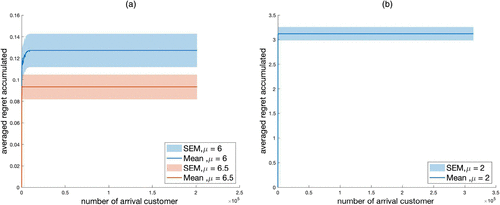
Notes. We set C = 1, , and . (a) λ = 1, R = 1, and the optimal threshold is . (b) λ = 1, , and the optimal thresholds {4, 5} ().
6.2. Expected Regret with Zero Being an Optimal Threshold
Figure 2(a) shows how the regret changes with respect to the number of arrivals for and when and λ = 1. The regret is averaged over 2,000 simulations, and there are more than 105 customers arrived in the system. In both cases shown in Figure 2(a), the genie-aided dispatcher uses threshold . Figure 2(b) shows the regret plot with respect to the number of customers for μ = 1 and λ = 1 when . The regret is averaged over 2,000 simulations, and there are more than customers arrived in the system. In this case, the optimal threshold is not unique: both and are optimal thresholds. The alternating genie-aided dispatcher uses the policy that is described in Proposition 11 and only changes the threshold between busy cycles. The plots indicate that sublinear regret is accumulated in all cases. Here, when the learning dispatcher uses threshold zero in phase 2 of a given batch, the existence of the forced exploration phase in the next batch results in regret being accumulated. Note that, for all plots shown in Figure 2, the optimal thresholds can be used by the learning dispatcher in phase 2 right from the first batch.
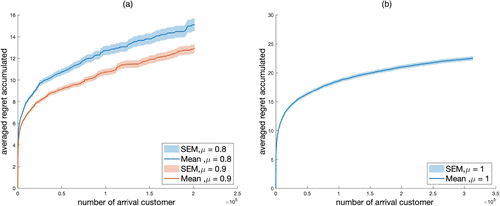
Notes. We set and . (a) λ = 1, and the optimal threshold is . (b) λ = 1, and the optimal thresholds are {0, 1}; .
6.3. Expected Regret with Different Choices of
We introduce truncation with the parameter in our analysis because we need a bound on the worst case queue length for the learning system. We obtained a particular order of the regret with the choice of . Next, we explore the impact of different choices of in Figure 3. We use ∼ to indicate the order at which increases: specifically, means . The regret values are averaged over 2,000 simulations, and there are more than arrival customers that arrive in more than 700 batches. In Figure 3, we use μ = 3, , and R = 21. The optimal threshold is . The queue with μ = 3 and is not stable. Despite this, Figure 3(b) suggests that constant regret is achieved for various truncation choices. However, when no truncation is enforced, the regret accumulated seems to grow linearly with respect to the number of arrivals; see Figure 3(a). This suggests that the truncation helps to ensure a lower regret, yet one may use a that grows faster than . Confirming this through analysis is a topic to explore in future research.
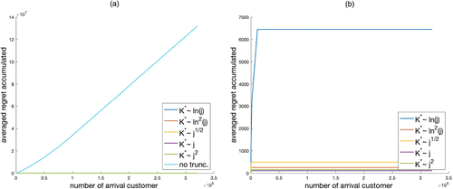
Notes. We set and . (a) With the no-truncation option included. (b) Excluding the no-truncation option.
6.4. Expected Regret with Different Choices of αj
We introduce to be the minimum length of phase 2 for the jth batch. Figure 4 plots the average regret accumulated with different choices of αj’s. In particular, Figure 4(a) is the log versus log-log plot of the regret accumulated when , λ = 1 with more than arrival customers, and Figure 4(b) plots the regret accumulated when μ = 3, with more than arrival customers. We use to denote . The regret is averaged over 2,000 simulations in both plots. Figure 4 suggests that, for all these choices of αj, a sublinear regret is accumulated, and having an αj that grows slower may still be able to achieve the regret bounds proved for .
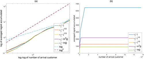
Notes. We set and . (a) Log versus log-log regret plot on regret accumulated when , λ = 1, and R = 1. Optimal threshold is . (b) Regret accumulated when μ = 3, , and R = 21. Optimal threshold is .
6.5. Expected Regret with Different Choices of
We also examine difference choices of , which controls the probability of having a phase 1 when the threshold used in the previous phase 2 is zero. Figure 5 shows the plots of various choices of . From these finite-time experiments, it seems that having a high enough chance to explore during the first few batches the learning dispatcher observes helps to reduce the regret accumulated. However, comparing the plots of and in Figure 5(a), it seems that only having a high probability of exploration for the first few batches is not enough to achieve O(1) regret because the slope of the plot for decreases a lot faster than the plot of . Although all the choices of seem to achieve sublinear regret for the case , always having the exploration phase when the threshold used in the previous phase 2 is zero accumulates a higher regret with a different scaling behavior.
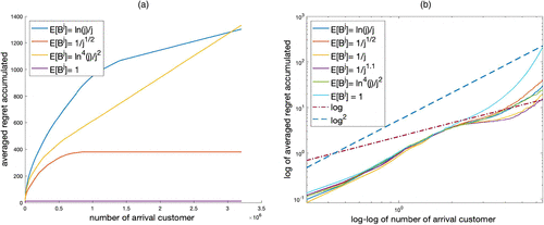
Notes. We set and . (a) Average regret plot when , λ = 1. The optimal threshold is . (b) Log versus log-log regret plot when , λ = 1. The optimal threshold is .
6.6. Expected Regret with Different Values of μ and λ
Figure 6 plots the average regret accumulated when seeing more than arriving customers when fixing one of the pair of arrival and service rates and varying the other. The regret values are averaged over 600 simulations. From the plot, we observe that, when the arrival rate is fixed, as the service rate increases, in general, the regret decreases. However, the decrease is not strict and instead is nonmonotonic, and the large cusps are usually around the parameter choices that have nonunique optimal thresholds. When the service rate is fixed, as the arrival rate increases, the regret follows a similar increasing/decreasing trend.
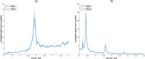
Notes. We set , and . (a) Average regret plot versus various λ’s when μ = 6. (b) Average regret plot versus various μ’s when λ = 1.
6.7. Comparison with Benchmark Algorithms
We also compare the finite time performance of our proposed Algorithm 1 with a few benchmark algorithms. In Figures 7 and 8, we compared Algorithm 1 with the estimate-then-optimize (ETO) and UCB algorithms when there are more than arrival customers and the regrets are averaged over 2,000 simulations. We use ETO(M) to denote the ETO algorithm that always accepts the first M customers. We use the UCB algorithm described in Lattimore and Szepesvári (2020, section 7.1) but with UCB bias subtracted from the estimated average service time. Figure 7(a) plots the log of average regret for the case when , λ = 1 and the optimal threshold is zero. Figure 7(b) plots the log of average regret for the case when μ = 3, , and the optimal threshold is eight. For the parameters used in these two plots, the optimal threshold is unique. Figure 8(a) plots the average regret for the case when μ = 1, λ = 1, and the optimal thresholds are {1, 0}. Figure 8(b) plots the average regret for the case when μ = 2, λ = 1, and the optimal thresholds are {5, 4}. For the parameter choices in Figure 8, the optimal threshold is not unique. The regret values in these two plots are computed with respect to the alternating genie-aided system that would change the threshold used between according to the threshold used by Algorithm 1, ETO, or UCB.
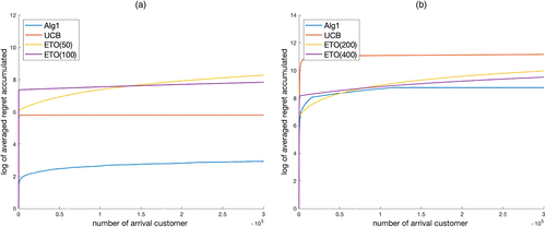
Notes. Alg1 is the learning algorithm proposed in Algorithm 1. We set , and . ETO(M) is the estimate-then-optimize algorithm that always accepts the first M customers. UCB is the upper confidence bound algorithm. (a) Log average regret plot when , λ = 1, R = 1, and . (b) Log average regret plot when μ = 3, , R = 21, and .
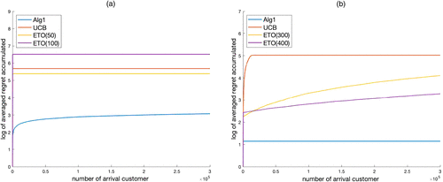
Notes. Alg1 is the learning algorithm proposed in Algorithm 1. We set C = 1, , and . ETO(M) is the estimate-then-optimize algorithm that always accepts the first M customers. UCB is the upper confidence bound algorithm. (a) Log averaged regret plot when μ = 1 and λ = 1. Both and are optimal thresholds. (b) Log of average regret plot when μ = 2, λ = 1, and R = 129/32. Both and are optimal thresholds.
The order of the regret accumulated by Algorithm 1 and UCB are similar in Figures 7(b) and 8(b). However, in Figures 7(a) and 8(a) in which zero is an optimal threshold, UCB achieves constant regret, yet Algorithm 1 achieves a sublinear regret. It is likely that the regret accumulated by Algorithm 1 would slowly increase as the number of arrivals increases and eventually becomes larger than the regret of the UCB algorithm. Our algorithm may choose to use threshold zero, and then a phase 1 may be enforced, and regret accumulates because of this. In Figure 9, we compare the finite time performance of our proposed algorithm with UCB when and λ = 1 with 2,000 simulations and more than 106 arrival customers. In this case, one is the unique optimal threshold. As we can observe from Figure 9, the regret of UCB increases in a (approximately) linear fashion, whereas our proposed algorithm is able to achieve constant regret. In fact, we can argue the following for UCB-based dispatching (under the simpler setting of the arrival rate being known):
When the optimal threshold(s) is positive, then some bad initial service time samples can result in the estimated threshold being zero. This bad event happens with positive probability for all (the probability decreases to zero as ). Whenever this bad event occurs, then the UCB-based dispatching algorithm stops dispatching customers, obtains no new service time samples, and incurs linear regret.
When zero is an optimal threshold, then the corresponding bad event of estimating the threshold as positive is more benign. This holds as dispatching more customers only results in more service-time samples, which then help to correct inaccurate estimates. Hence, we expect to achieve a constant or slowly growing (sublinear) regret.
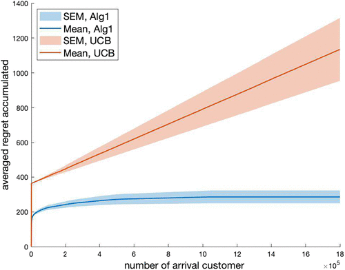
Notes. Alg1 is the learning algorithm proposed in Algorithm 1. We set and . UCB is the upper confidence bound algorithm.
Note that this explanation supports the conjecture in Remark 5 because the worst case (over parameters) regret of UCB is expected to be linear in N. Moreover, because UCB needs to compute the estimated threshold at every arrival, it requires more computation when compared with Algorithm 1.
6.8. Comparison of Different Genie-Aided Algorithms
Figure 10 compares the accumulated net gain between the alternating genie-aided algorithm (“AG algo” in the legend) coupled with Algorithm 1 and the genie-aided algorithms using threshold (“ThreshK algo” in the legend) or (“ThreshK-1 algo” in the legend) when optimal thresholds are not unique; the accumulated net gain of the genie-aided algorithm using threshold are scaled to be zero. Figure 10 plots the difference between the net gain obtained by the alternating genie-aided system and the genie-aided system using static threshold and the difference of the net gain between two genie-aided systems using static threshold and over two sets of parameters. We also include the regret accumulated by the learning algorithm compared with the genie-aided algorithm using threshold K − 1. The performances of the algorithms are averaged over 18,000 simulations. As we can observe from the plots, the regret accumulated by the learning algorithm (with respect to either the alternating genie-aided system or the genie-aided system using threshold K − 1) dominates the performance difference between the alternating genie-aided system and the genie-aided system using threshold K − 1, and the performing difference between the genie-aided system using threshold K and the genie-aided system using threshold K − 1. This is more evidence in favor of Remark 6.
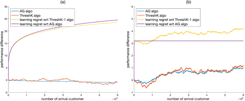
Notes. The accumulated net gain of the genie algorithm using threshold is scaled to be zero. (a) . Both and are optimal thresholds. (b) μ = 2, λ = 1, and R = 129/32. Both and are optimal thresholds.
7. Conclusions
In this paper, we considered a social welfare–maximizing problem, which was first proposed and studied in Naor (1969). We studied the learning problem of finding the proper threshold admission policy when the service and arrival rates are unknown. We proposed a learning algorithm that consists of batches in which each batch has an optional exploration phase with a fixed length and an exploitation phase. When the optimal policy is unique, we showed that our learning algorithm achieves an O(1) regret whenever the optimal threshold is nonzero and achieves an regret when the optimal threshold is zero, where N denotes the total number of arrival customers to the systems. When the optimal policy is not unique, we specified a particular optimal policy to compare with and proved that similar regret bounds hold for our learning algorithm.
In our analysis, we assumed Poisson arrivals and exponentially distributed services with fixed arrival and service rate. We want to adapt our algorithm to more general arrival processes and service-time distributions such as the models in Lippman and Stidham (1977) and Johansen and Stidham (1980) so that a small regret is obtained in these more general settings too, such as generalization to optimal admission control in an queue with our information structure. This problem has received attention—see Oz (2022)—under a different information structure in which only the queue length is observed by arrivals. Under this setting, the analytical optimal strategy for this problem is still unknown and may be time-varying; see Oz (2022) for details. However, the problem may be tractable with our information structure as the Markov state—number in service and service time elapsed of customer currently being served—is observable and MDP theory could be applied. Another possible direction is to consider a single queue with a buffer but with multiple servers as in the model in Knudsen (1972). Again, the aim would be to adapt our current learning algorithm to this setting as well, achieving low regret. Finally, we conjectured that the order of the regret accumulated for the worst case choice of parameters would grow at least as ; see Remark 5. Proving (or disproving) this conjecture is yet another problem for future work.
The authors are grateful to the associate editor and two anonymous referees for valuable comments on an earlier version of the paper.
1 We show how to translate the regret from the number of arrivals to a time horizon.
2 We discuss what we mean by “optimal” in Remark 6 after we specify the strategy to which we compare our learning algorithm in the case that there are multiple optimal thresholds.
References
- (2022) Learning a discrete set of optimal allocation rules in queueing systems with unknown service rates. Preprint, submitted February 4, https://arxiv.org/abs/2202.02419.Google Scholar
- (2022) Learning in structured MDPs with convex cost functions: Improved regret bounds for inventory management. Oper. Res. 70(3):1646–1664.Link, Google Scholar
- (2022) Scheduling in the high uncertainty heavy traffic regime. Preprint, submitted April 12, https://arxiv.org/abs/2204.05733.Google Scholar
- (2014) Sharp finite-time iterated-logarithm martingale concentration. Preprint, submitted May 12, https://arxiv.org/abs/1405.2639.Google Scholar
- (2019) Reinforcement Learning and Optimal Control (Athena Scientific, Belmont, MA).Google Scholar
- (1985) The rule revisited. Adv. Appl. Probab. 17(1):237–238.Google Scholar
- (2020) Knowledge, congestion, and economics: Parameter uncertainty in Naor’s model. Queueing Systems 96(1–2):83–99.Google Scholar
- (2023) An online learning approach to dynamic pricing and capacity sizing in service systems. Oper. Res., ePub ahead of print June 12, https://doi.org/10.1287/opre.2020.612.Google Scholar
- (2021) Job dispatching policies for queueing systems with unknown service rates. Proc. 22nd Internat. Sympos. Theory Algorithmic Foundations Protocol Design Mobile Networks Mobile Comput. (Association for Computing Machinery, New York), 181–190.Google Scholar
- (2019a) Asymptotic analysis of a multiclass queueing control problem under heavy traffic with model uncertainty. Stochastic Systems 9(4):359–391.Link, Google Scholar
- (2019b) Brownian control problems for a multiclass M/M/1 queueing problem with model uncertainty. Math. Oper. Res. 44(2):739–766.Link, Google Scholar
- (2021) Asymptotic optimality of the generalized rule under model uncertainty. Stochastic Processes Appl. 136:206–236.Google Scholar
- (1961)
Queues . Methuen’s Monographs on Statistical Subjects, Methuen & Co., Ltd., London (John Wiley & Sons, Inc., New York).Google Scholar - (1968) On the strong law of large numbers and the central limit theorem for martingales. Trans. Amer. Math. Soc. 131:259–275.Google Scholar
- (2016) Essentials of Stochastic Processes, Springer Texts in Statistics (Springer, Cham, Switzerland).Google Scholar
- (2022) Online learning and pricing for service systems with reusable resources. Oper. Res., ePub ahead of print November 10, https://doi.org/10.1287/opre.2022.2381.Link, Google Scholar
- (1980) Control of arrivals to a stochastic input-output system. Adv. Appl. Probab. 12(4):972–999.Google Scholar
- (1972) Individual and social optimization in a multiserver queue with a general cost-benefit structure. Econometrica 40:515–528.Google Scholar
- (2018a) On learning the cµ rule in single and parallel server networks. Preprint, submitted February 2, https://arxiv.org/abs/1802.06723.Google Scholar
- (2021) Learning unknown service rates in queues: A multiarmed bandit approach. Oper. Res. 69(1):315–330.Link, Google Scholar
- (2018b) Augmenting max-weight with explicit learning for wireless scheduling with switching costs. IEEE/ACM Trans. Networking 26(6):2501–2514.Google Scholar
- (2020) Bandit Algorithms (Cambridge University Press, Cambridge, UK).Google Scholar
- (1977) Individual vs. social optimization in exponential congestion systems. Oper. Res. 25(2):233–247.Link, Google Scholar
- (1969) The regulation of queue size by levying tolls. Econometrica 37(1):15–24.Google Scholar
- (2012) Max-weight learning algorithms for scheduling in unknown environments. IEEE Trans. Automatic Control 57(5):1179–1191.Google Scholar
- (2022) Optimal admission policy to an observable M/G/1 queue. Queueing Systems 100(3–4):477–479.Google Scholar
- (1986)
An optimal adaptive scheme for two competing queues with constraints . Bensoussan FA, Lions JL, eds. Analysis and Optimization of Systems, vol. 83 (Springer, Berlin), 515–532.Google Scholar - (1956) Various optimizers for single-stage production. Naval Res. Logist. Quart. 3:59–66.Google Scholar
- (2021) Learning algorithms for minimizing queue length regret. IEEE Trans. Inform. Theory 67(3):1759–1781.Google Scholar
- (2018) Reinforcement Learning: An Introduction, 2nd ed., Adaptive Computation and Machine Learning (MIT Press, Cambridge, MA).Google Scholar
- (2009) Explicit probability density function for the length of a busy period in an M/M/1/K queue. Yue W, Takahashi Y, Takagi H, eds. Advances in Queueing Theory and Network Applications (Springer, New York), 213–226.Google Scholar
- (2018) High-Dimensional Probability, Cambridge Series in Statistical and Probabilistic Mathematics, vol. 47 (Cambridge University Press, Cambridge, UK).Google Scholar
- (2019) High-Dimensional Statistics, Cambridge Series in Statistical and Probabilistic Mathematics, vol. 48 (Cambridge University Press, Cambridge, UK).Google Scholar
- (2021) Learning and information in stochastic networks and queues. Preprint, submitted May 18, https://arxiv.org/abs/2105.08769.Google Scholar
- (2023) Learning while scheduling in multi-server systems with unknown statistics: MaxWeight with discounted UCB. Ruiz F, Dy J, van de Meent JW, eds. Proc. 26th Internat. Conf. Artificial Intelligence Statist., vol. 206 (PMLR, New York), 4275–4312.Google Scholar
- (2022) Learning the scheduling policy in time-varying multiclass many server queues with abandonment. Preprint, submitted May 9, https://dx.doi.org/10.2139/ssrn.4090021.Google Scholar