Smoothed Variable Sample-Size Accelerated Proximal Methods for Nonsmooth Stochastic Convex Programs

1. Introduction

We consider the following stochastic nonsmooth convex optimization problem:

where $f(x)\triangleq \mathbb{E}[\tilde{f}(x,\xi (\omega ))],\hspace{0.17em}\xi :\mathrm{\Omega }\to {\mathbb{R}}^o,\hspace{0.17em}\tilde{f}:{\mathbb{R}}^n\times {\mathbb{R}}^o\to \mathbb{R}$; g is a closed, convex, and proper deterministic function with an efficient proximal evaluation; $(\mathrm{\Omega },\mathcal{H},\mathbb{P})$ denotes the associated probability space; and $\mathbb{E}[•]$ denotes the expectation with respect to the probability measure $\mathbb{P}$. Throughout, we refer to $\tilde{f}(x,\xi (\omega ))$ by $\tilde{f}(x,\omega )$, whereas $\tilde{F}(x,\omega )\triangleq \tilde{f}(x,\omega )+g(x)$. We consider settings in which $\tilde{f}(·,\omega )$ is nonsmooth strongly convex/convex in x for every ω, generalizing the focus beyond the structured nonsmooth setting in which the “stochastic part” is smooth. Specifically, structured nonsmooth problems require minimizing $f(x)+g(x)$, where f is smooth, whereas g is nonsmooth with an efficient prox evaluation (allows for capturing constrained problems over closed and convex sets).

Among the earliest avenues for resolving (1) is stochastic approximation (Robbins and Monro 1951, Kushner and Yin 2003), and it is proven to be effective on a breadth of stochastic computational problems, including convex optimization problems. Polyak and Juditsky (1992) develop an averaging scheme in convex differentiable settings, deriving the optimal convergence rate of $\mathcal{O}(1/\sqrt{K})$ under classic assumptions, where k is the number of iterations. Among the cleanest of early complexity requirements for the minimization of expectation-valued μ-strongly convex and convex functions over a closed and convex set X are given as $\left(\max \left\{\frac{M^2}{{\mu }^2},\Vert x_0-x^{*}{\Vert }^2\right\}\frac{1}{ϵ}\right)$ (to ensure that $\mathbb{E}[\Vert x_k-x^{*}{\Vert }^2]\le ϵ$) and $\mathcal{O}\left(\frac{M{D}_X}{{ϵ}^2}\right)$ (to ensure that the expected optimality gap is less than ϵ), respectively, where $S(x,\omega )$ denotes a measurable selection from ${\partial }_x\tilde{f}(x,\omega )$, ${\sup }_{x\in X}\mathbb{E}[\Vert S(x,\omega ){\Vert }^2]\le M^2$, and $D_X\triangleq {\max }_{x\in X}\Vert x_0-x\Vert$. Of these, the former is presented by Shapiro et al. (2009), whereas the latter is the result of an optimal robust constant step length stochastic approximation scheme suggested by Nemirovski et al. (2009). When f is both L-smooth and μ-strongly convex, an improved complexity requirement (from a constant factor standpoint) of $\mathcal{O}\left(\sqrt{\frac{L\Vert x_0-x^{*}{\Vert }^2}{ϵ}}+\frac{{\nu }^2}{\mu ϵ}\right)$ is provided by Ghadimi and Lan (2013). This contrasts sharply with the deterministic regime in which $\mathcal{O}(\log (1/ϵ))$ and $\mathcal{O}(1/\sqrt{ϵ})$ steps are required in smooth strongly convex and smooth convex regimes to compute an ϵ-accurate solution (ϵ-solution in terms of mean squared error) and ϵ-optimal solution (ϵ-solution in terms of expected suboptimality), respectively. In structured nonsmooth regimes, there is an effort to employ the stochastic generalization of an accelerated proximal gradient method to minimize $f+g$ when f is smooth. Reliant on a first order oracle that produces a sampled gradient ${\nabla }_x\tilde{f}(x,\omega )$ and given an x₀, our proposed variable sample-size accelerated proximal gradient scheme (VS-APM) (also see Ghadimi and Lan 2016, Jofré and Thompson 2017) is stated as follows in which the true gradient is replaced by a sample average $({\nabla }_{x}f(x_k)+{\overline{w}}_{k,N_k})$ with batch size N_k.

where ${\overline{w}}_{k,N_k}\triangleq \frac{{\sum }_{j=1}^{N_k}({\nabla }_x\tilde{f}(x_k,{\omega }_{j,k})-{\nabla }_{x}f(x_k))}{N_k},\hspace{0.17em}{\mathbf{P}}_{\eta g}(y)\triangleq \arg {\min }_x\left\{\frac{1}{2}\Vert x-y{\Vert }^2+\frac{1}{2\eta }g(x)\right\}$, γ_k, and β_k are suitably defined step lengths. Our approach produces linearly convergent iterates in strongly convex regimes and achieves an iteration complexity of $\mathcal{O}(1/K^2)$ in merely convex and smooth regimes, where K is the total number of iterations, matching the deterministic results seen in the work by Beck and Teboulle (2009) and Nesterov (1983). The avenue represented by (2) has two key distinctions: (i) increasingly exact gradients through increasing batch sizes N_k of sampled gradients, allowing for progressive variance reduction, and (ii) larger (nondiminishing) step sizes in accordance with deterministic accelerated schemes. Collectively, (i) and (ii) allow for recovering fast (i.e., deterministic) convergence rates (in an expected value sense) when N_k grows sufficiently fast. Additionally, such schemes have a more muted reliance on the condition number $\kappa =L/\mu$ (in μ-strongly convex and L-smooth regimes); specifically, in accelerated schemes, such dependence reduces to $\sqrt{\kappa }$ in comparison with κ in unaccelerated counterparts (cf. Nesterov 2014).

1.1. Prior Research

1.1.1. Stochastic Gradient Schemes.

In nonsmooth convex stochastic optimization problems, Nemirovski et al. (2009) derive an optimal rate of $\mathcal{O}(1/\sqrt{K})$ in terms of expected suboptimality via an optimal constant step length (also see Shamir and Zhang 2013), whereas in strongly convex regimes, they derive a rate of $\mathcal{O}(1/K)$ in a mean squared sense. Structured nonsmooth problems (or composite problems) as defined by (1) are examined extensively (cf. Ghadimi and Lan 2012, Lan 2012), and rates of $\mathcal{O}(L/K^2+1/\sqrt{K})$ and $\mathcal{O}(L/K+1/\sqrt{K})$ are developed by Dang and Lan (2015) via a mirror-descent framework for strongly convex and convex problems with L-smooth objectives, respectively. In related work, Devolder et al. (2014) derive oracle complexities with a deterministic oracle of fixed inexactness, which is extended to a stochastic oracle by Dvurechensky and Gasnikov (2016). Randomized smoothing techniques are also employed by Yousefian et al. (2012) together with recursive step lengths (see Newton et al. 2018 for a review).

1.1.2. Variance Reduction.

In strongly convex regimes (without acceleration), a linear rate of convergence in expected error is first shown for variance-reduced gradient methods by Shanbhag and Blanchet (2015) and revisited by Jofré and Thompson (2017), whereas similar rates are provided for extragradient methods by Jalilzadeh and Shanbhag (2016); the accelerated counterpart (VS-APM) mutes the dependence on κ, improving the bound to $\mathcal{O}(\sqrt{L/\mu }\log (1/ϵ))$. In smooth regimes, an accelerated scheme is first presented by Ghadimi and Lan (2016), in which every iteration requires two prox evaluations, admitting the optimal iteration complexity and oracle complexity of $\mathcal{O}(1/\sqrt{ϵ})$ and $\mathcal{O}(1/{ϵ}^2)$, respectively. Jofré and Thompson (2017) extend this scheme to allow for state-dependent noise. An extragradient-based variable sample-size framework is suggested by Jalilzadeh and Shanbhag (2016) with a rate of $\mathcal{O}(1/K)$.

1.1.3. Smoothing Techniques for Nonsmooth Problems.

For a subclass of deterministic nonsmooth problems, Nesterov (2005b) proves that an ϵ-optimal solution is computable in $\mathcal{O}(1/ϵ)$ gradient steps by applying an accelerated method to a smoothed problem (primal smoothing with fixed smoothing parameter). Subsequently, Nesterov (2005a) considers primal–dual smoothing in deterministic regimes (extended to composite problems by Tran-Dinh et al. 2018) with a diminishing smoothing parameter, leading to rates of $\mathcal{O}(1/K^2)$ and $\mathcal{O}(1/K)$ for strongly convex and convex deterministic problems, respectively (also see Devolder et al. 2012, Boţ and Hendrich 2013). Adaptive smoothing, considered by Tran-Dinh (2017), is shown to have an iteration complexity of $\mathcal{O}(1/ϵ)$, whereas Ouyang and Gray (2012) show that smoothing-based minimization of $\mathbb{E}[\tilde{f}(x,\omega )]+\mathbb{E}[\tilde{g}(x,\omega )]$ leads to rates $\mathcal{O}(1/K)$ and $\mathcal{O}(1/\sqrt{K})$ when $\tilde{g}(·,\omega )$ is nonsmooth for almost every (a.e.) ω, whereas $\tilde{f}(·,\omega )$ is either strongly convex or merely convex for a.e. ω (extended by Zhong and Kwok 2014).¹

1.2. Gaps and Contributions

Unfortunately when $\tilde{f}(·,\omega )$ is a nonsmooth strongly convex/convex function, stochastic subgradient schemes (subsequently defined in (SSG)), while a de facto standard, generally display poor empirical behavior because they utilize diminishing step lengths and noisy gradients. We develop two distinct avenues for combining smoothing with acceleration and variance reduction in strongly convex and convex regimes that ameliorate these concerns while achieving optimal rates.

1.2.1. mVS-APM for Strongly Convex Nonsmooth f.

In Section 2, our smoothing framework is reliant on a variable sample-size accelerated proximal method (VS-APM), which requires smoothness of f while displaying linear convergence and optimal oracle complexity. In two distinct settings, we propose applying VS-APM (or an unaccelerated variant) on the Moreau envelope of F, denoted by $F_{\eta }$, where $F_{\eta }$ is $\frac{1}{\eta }$-smooth and retains the minimizers of F.

1.2.1.1. Compact Domains.

Under the assumption that the domain of g is bounded and $\mathbb{E}[\Vert S(x,\omega ){\Vert }^2]\le M^2$ for all $x\in {\mathbb{R}}^n$, where $S(x,\omega )$ is a measurable selection from $\partial \tilde{f}(x,\omega )$; i.e. $S(x,\omega )\in \partial \tilde{f}(x,\omega )$, we show that (mVS-APM) produces a linearly convergent sequence with an iteration complexity of $\mathcal{O}(\log (1/ϵ))$ in inexact gradient steps ${\nabla }_x{F}_{\eta }(x_k)$, where increasingly exact gradients ${\nabla }_x{F}_{\eta }(x)$ are obtained by employing a (prox-SSG) scheme. In particular, our variance-reduced scheme endeavors to get increasingly exact gradients by progressively reducing the bias in the gradients (because we utilize an increasing number of SSG steps); such a benefit does not appear in a naive implementation of SSG. Moreover, the overall complexity in subgradient evaluations (and consequently sample or oracle complexity) is $\mathcal{O}(1/ϵ)$, matching the optimal complexity in subgradient steps achieved by (SSG) schemes.

1.2.1.2. Unbounded Domains.

When domains are possibly unbounded, assuming that $\mathbb{E}[\Vert S(x,\omega ){\Vert }^2]\le {\overline{M}}^2\Vert x{\Vert }^2+M^2$, where $S(x,\omega )\in \partial \tilde{F}(x,\omega )$, the proposed (unaccelerated) variable sample-size proximal method (mVS-PM) achieves an iteration complexity of $\mathcal{O}(\log (1/ϵ))$ (in gradient steps with ${\nabla }_x{F}_{\eta }$) and overall complexity in subgradient steps of $\mathcal{O}(1/ϵ)$.

1.2.2. sVS-APM for Convex Nonsmooth f.

In this setting, in Section 3, we develop an iterative smoothing-based extension of VS-APM, denoted by sVS-APM. By reducing the smoothing and step length parameters at a suitable rate, $\mathbb{E}[F(y_K)-F(x^{*})]\le \mathcal{O}(1/K)$. Notably sVS-APM produces asymptotically accurate solutions (unlike the scheme by Nesterov (2005b), which produces approximate solutions via a fixed smoothing parameter) and is characterized by the optimal oracle complexity of $\mathcal{O}(1/{ϵ}^2)$. When f is convex and smooth, we may specialize these results to obtain an optimal rate of $\mathcal{O}(1/K^2)$ and display an optimal sample complexity of $\mathcal{O}(1/{ϵ}^2)$. When f is deterministic but nonsmooth, s-APM matches the rate by Nesterov (2005b) but produces asymptotically exact solutions. Additionally, we prove that, for suitable (but distinct) choices of step length and smoothing sequences, sVS-APM and VS-APM produce sequences that converge almost surely (a.s.) to a solution of (1), a convergence statement that was unavailable thus far, matching deterministic results by Orabona et al. (2012) and Boţ and Hendrich (2015) that leverage Moreau smoothing; we provide a result for $(\alpha ,\beta )$-smoothable functions (see Beck 2017).

1.2.3. Notation.

A vector x is assumed to be a column vector, whereas $\Vert x\Vert$ denotes the Euclidean vector norm, that is, $\Vert x\Vert =\sqrt{x^{T}x}$. ${\mathbf{P}}_{\eta g}(x)$ denotes the prox with respect to g with prox parameter $\frac{1}{2\eta }$ at x. $\mathbb{E}[z]$ denotes the expectation of a random variable z. We let $X^{*}$ denote the set of optimal solutions of (1).

2. Nonsmooth Strongly Convex Problems

In this section, we develop rate and complexity analysis for nonsmooth strongly convex optimization problems via techniques that combine smoothing, acceleration, and variance reduction. In Section 2.1, we review a linearly convergent variance-reduced accelerated proximal scheme (VS-APM) for smooth stochastic convex optimization; this scheme serves as our subproblem solver. In Section 2.2, we present a Moreau-smoothed variant of VS-APM, referred to as (mVS-APM), which relies on minimizing the Moreau envelope $F_{\eta }$ of the strongly convex nonsmooth function F by VS-APM. In Section 2.3, we then derive rate and complexity guarantees for (mVS-APM), where ${\nabla }_x{F}_{\eta }$ is approximated with increasing accuracy by a stochastic subgradient (SSG) scheme. Finally, in Section 2.4, we derive analogous statements when applying an unaccelerated variable sample-size proximal method (mVS-PM) under possibly non-compact domains and under a (weaker) state-dependent bound on the subgradient (see Table 1 for a summary of findings).

Table 1. Comparison of Schemes in Nonsmooth (NS) and Strongly Convex Regimes in Terms of Convergence Rate and Complexity of Iterations, Proximal Evals., and Oracle Evaluations ($\kappa =L/\mu$), Where $\rho \in (0,1)$

2.1. Background on VS-APM

Consider (1), in which f, g, and the initial point x₀ satisfy the following assumption.

Assumption 1.

(i) $f$ is a μ-strongly convex function, and g is a closed, convex, and proper deterministic function. (ii) There exist $C,D>0$ such that $\mathbb{E}[\Vert x_0-x^{\ast }{\Vert }^2]\le C$ and $\mathbb{E}[\Vert F(x_0)-F(x^{*})\Vert ]\le D$, where $F(x)\triangleq f(x)+g(x)$ and $x^{*}$ solves (1).

In a subset of regimes, we impose an L-smoothness assumption on f.

Assumption 2.

The function $f$ is continuously differentiable with a Lipschitz continuous gradient with constant L; i.e., $\Vert {\nabla }_{x}f(x)-{\nabla }_{x}f(y)\Vert \le L\Vert x-y\Vert$ for all $x,y\hspace{0.17em}\in \hspace{0.17em}{\mathbb{R}}^n.$

We utilize a variable sample-size accelerated proximal scheme (VS-APM) as defined in Algorithm 1, which can process such problems and differs from a standard accelerated proximal method in that we employ an inexact gradient ${\nabla }_{x}f(x_k)+{\overline{w}}_{k,N_k}$, where the bound on the second moment of ${\overline{w}}_{k,N_k}\triangleq {\nabla }_{x}f(x_k)-\frac{{\sum }_{k=0}^{N_k}{\nabla }_{x}f(x_k,{\omega }_k)}{N_k}$ is diminishing with k, a consequence of using variance reduction.

Algorithm 1

(Variable Sample-Size Accelerated Proximal Method)

• (0) Given $x_0$, y₀ = x₀, κ, and positive sequences $\{{\gamma }_k,N_k\}$, set ${\lambda }_1\in (1,\sqrt{\kappa }\hspace{0.17em}]$, $k≔1$.

• (1) $y_{k+1}≔{\mathbf{P}}_{{\gamma }_{k}g}(x_k-{\gamma }_k({\nabla }_{x}f(x_k)+{\overline{w}}_{k,N_k}))$.

• (2) ${\lambda }_{k+1}≔\frac{1}{2}\left(1-\frac{{\lambda }_k^2}{\kappa }+\sqrt{{(1-\frac{{\lambda }_k^2}{\kappa })}^2+4{\lambda }_k^2}\right)$.

• (3) $x_{k+1}≔y_{k+1}+\left(\frac{({\lambda }_k-1)(1-\frac{1}{4\kappa }{\lambda }_{k+1})}{(1-\frac{1}{4\kappa }){\lambda }_{k+1}}\right)(y_{k+1}-y_k)$.

• (4) If k > K, then stop; else $k≔k+1$; return to step 1.

We outline the assumptions on the first and second moments of ${\overline{w}}_k$.

Assumption 3.

(i) Conditional boundedness of second moments: there exists $\nu >0$ such that $\mathbb{E}[\Vert {\overline{w}}_k{\Vert }^2|{\mathcal{H}}_k]\le \frac{{\nu }^2}{N_k}$ holds a.s. for all k and ${\mathcal{H}}_k\triangleq \sigma \{x_0,x_1, \dots ,x_{k-1}\}$. (ii) Conditional unbiasedness of first moments: $\mathbb{E}[w_k|{\mathcal{H}}_k]=0$ holds a.s., where $w_k\triangleq {\nabla }_{x}f(x_k,{\omega }_k)-{\nabla }_{x}f(x_k)$.

VS-APM can be shown to achieve linear convergence akin to that by Nesterov (2014) by combining inexact gradients in which the inexactness is driven to zero by increasing the sample-size in estimating the gradients. This avenue also allows for achieving the optimal oracle complexity to obtain an ϵ-accurate solution. These differences lead to a slightly modified set of update rules in contrast with that developed by Nesterov (2014) and require that ${\gamma }_k=1/2L$ rather than $1/L$. This scheme serves as a subproblem solver in subsequent sections, and we now state a lemma and the associated complexity statement of VS-APM. The proof is similar to that by Nesterov (2014) and is in the appendix. Importantly, this scheme allows for a possibly biased estimate of the gradient.

Lemma 1.

Suppose Assumptions 1–3(i) hold. Consider the iterates generated by VS-APM, where ${\gamma }_k=\frac{1}{2L}$ for all $k\ge 0,\hspace{0.17em}\kappa =\frac{L}{\mu }$, and $\overline{\alpha }=\frac{1}{2\sqrt{\kappa }}$. Then, the following holds for all K.

$$\mathbb{E}[F(y_K)-F^{*}]\le \left(D+\frac{\mu }{2}{C}^2\right){(1-\overline{\alpha })}^{K-1}+{\displaystyle \sum _{i=0}^{K-1}\frac{{(1-\overline{\alpha })}^i\left(\frac{2}{L}+\frac{1}{\mu }\right){\nu }^2}{N_{k-i}}}+{\displaystyle \sum _{i=0}^{K-2}\frac{{(1-\overline{\alpha })}^{i+1}\left(\frac{2}{L}+\frac{1}{\mu }\right){\nu }^2}{N_{k-i-1}}}.$$(3)

The following theorem characterizes the iteration and oracle complexity of VS-APM.

Theorem 1

(Rate and Oracle Complexity of VS-APM Under Biased Oracles). Suppose Assumptions 1–3(i) hold. Consider the iterates generated by VS-APM, where ${\gamma }_k\triangleq \frac{1}{2L},\hspace{0.17em}{N}_k\triangleq \lfloor {\rho }^{-k}\rfloor ,\hspace{0.17em}\theta \triangleq \left(1-\frac{1}{2\sqrt{\kappa }}\right),\hspace{0.17em}\rho \triangleq \left(1-\frac{1}{2a\sqrt{\kappa }}\right)$ for all $k\ge 0$ and a > 2.

1. $\mathit{For} \mathit{all} K, we \mathit{have} \mathit{that} \mathbb{E}[F(y_K)-F^{*}]\le \tilde{C}{\rho }^{K-1} \hspace{0.17em}\hspace{0.17em}\mathit{where}\hspace{0.17em}\hspace{0.17em} \tilde{C}\triangleq \left(D+\frac{\mu }{2}{C}^2\right)+\frac{4{\nu }^2}{\mu }+\frac{2{\nu }^2\sqrt{\kappa }}{\mu }.$  (4)

   In addition, VS-APM needs $\mathcal{O}(\sqrt{\kappa }\log (\frac{1}{ϵ}))$ steps to obtain an ϵ-accurate solution, that is, $\mathbb{E}[F(y_{K+1})-F^{*}]\le ϵ$.

2. To compute an ϵ-accurate solution, ${\displaystyle {\sum }_{k=1}^K{N}_k}\le \left(\left(D+\frac{\mu C^2}{2}\right)+\frac{4{\nu }^2}{\mu }+\frac{2{\nu }^2\sqrt{\kappa }}{\mu }\right)\mathcal{O}\left(\frac{\sqrt{\kappa }}{ϵ}\right).$

We know of no other result for variance-reduced accelerated proximal schemes in strongly convex (or even convex) smooth regimes that allows for biased oracles. For instance, Schmidt et al. (2011) impose unbiasedness in strongly convex regimes. Next, we show that adding the unbiasedness requirement, that is, $\mathbb{E}[w_k|{\mathcal{H}}_k]=0$ a.s. for all k improves the constants in these bounds.

Corollary 1

(Rate and Oracle Complexity of VS-APM Under Unbiased Oracles). Suppose Assumptions 1–3(i,ii) hold. Consider the iterates generated by VS-APM, where ${\gamma }_k\triangleq \frac{1}{2L},\hspace{0.17em}{N}_k\triangleq \lfloor {\rho }^{-k}\rfloor ,\hspace{0.17em}\theta \triangleq \left(1-\frac{1}{2\sqrt{\kappa }}\right),\hspace{0.17em}\rho \triangleq \left(1-\frac{1}{2a\sqrt{\kappa }}\right)$ for all $k\ge 0$ and a > 2.

1. $\mathit{For} \mathit{all} K, we \mathit{have} \mathit{that} \mathbb{E}[F(y_K)\text{−}{F}^{*}]\le \tilde{C}{\rho }^{K\text{-}1} \mathit{where} \hspace{0.17em}\tilde{C}\triangleq \left(D+\frac{\mu }{2}{C}^2\right)+\frac{4{\nu }^2}{\mu }.$(5)

   In addition, VS-APM needs $\mathcal{O}(\sqrt{\kappa }\log (1/ϵ))$ steps to obtain an ϵ-accurate solution.

2. To compute an ϵ-accurate solution, ${\sum }_{k=1}^K{N}_k\le \left(\left(D+\frac{\mu C^2}{2}\right)+\frac{4{\nu }^2}{\mu }\right)\mathcal{O}\left(\frac{\sqrt{\kappa }}{ϵ}\right).$

The application of VS-APM is afflicted by the need for the L-smoothness of f as well as the availability of L, the Lipschitz constant. Naturally, in many settings, the problem may not be smooth, and even if L-smoothness holds, an estimate of L may be unavailable. Consequently, to broaden the reach of the scheme, an approach that obviates the need for L or the imposition of the smoothness assumption is necessitated. This prompts the subsequent smoothed scheme, (mVS-APM). This scheme can always be implemented if the strong convexity modulus (denoted by μ) is known but the function is either nonsmooth or smooth with an unknown Lipschitz constant L. It is worth noting that estimating μ is challenging, and if μ is indeed unknown, then in Section 3, we introduce an iteratively smoothed VS-APM (sVS-APM) method that necessitates neither the knowledge of the Lipschitz constant L nor the smoothness of f nor the strong convexity modulus μ.

2.2. A Moreau-Smoothed Inexact Accelerated Framework (mVS-APM)

When $\tilde{f}(·,\omega )$ is a nonsmooth strongly convex function for almost every ω, then the standard approach lies in utilizing stochastic subgradient schemes (SSG) in which convergence relies on choosing square-summable but nonsummable step length sequences. The choice of the parameters in such sequences can have a debilitating impact on performance in some settings (cf. Shapiro et al. 2009). Specifically, choosing γ_k as $1/(\mu \lambda \mathrm{)}$ minimizes the mean squared error but overestimating μ can have catastrophic impact as seen in Shapiro et al. (2009, section 5.9, example 5.36). More generally, such choices are often characterized by poor asymptotic behavior, a consequence that arises in part from the diminishing nature of step length sequences and the noisy subgradients. We consider a distinct avenue reliant on minimizing the Moreau envelope of a closed, convex, and proper function F (cf. Moreau 1965), denoted by $F_{\eta }$ and defined next.

Notably, this smoothing retains the minimizer of F when F is strongly convex.

Lemma 2

(Planiden and Wang 2016, Lemma 2.19). Consider a convex, closed, and proper function F and its Moreau envelope $F_{\eta }(x)$. Then, the following hold: (i) $x^{*}$ is a minimizer of F over ${\mathbb{R}}^n$ if and only if $x^{*}$ is a minimizer of $F_{\eta }$; (ii) F is μ-strongly convex on ${\mathbb{R}}^n$ if and only if $F_{\eta }$ is $\overline{\mu }$-strongly convex on ${\mathbb{R}}^n$, where $\overline{\mu }\triangleq \frac{\mu }{\eta \mu +1}$.

Consequently, we minimize the $\overline{\mu }$-strongly convex and $\frac{1}{\eta }$-smooth function $F_{\eta }$, which is not necessarily an easy task because computing ${\nabla }_x{F}_{\eta }(x)$ necessitates solving nonsmooth stochastic optimization problems. We adopt an inexact accelerated proximal scheme for minimizing $F_{\eta }$. But, in contrast with (SSG) schemes applied to minimizing F, we control the smoothness of the outer problem by choosing η and utilize (i) larger nondiminishing step lengths, (ii) acceleration, and (iii) increasingly exact gradients, all of which are distinct from (SSG), as shown next.

Importantly, ${\nabla }_x{F}_{\eta }(x_k)+{\overline{w}}_{k,N_k}$ represents an approximation of the gradient of the Moreau envelope. The true gradient of the Moreau envelope $F_{\eta }$ is defined as ${\nabla }_x{F}_{\eta }(x)=\frac{1}{\eta }(x-{\text{prox}}_{\eta F}(x))$, where

But ${\text{prox}}_{\eta F}(x)$ cannot be computed in finite time because F is a nonsmooth, expectation-valued convex function. Instead, via stochastic approximation, we compute an approximate solution of ${\text{prox}}_{\eta F}(x)$ denoted by ${\widehat{\text{prox}}}_{\eta F}(x)$, implying that the inexact gradient of $F_{\eta }(x)$ is given by $\frac{1}{\eta }(x-{\widehat{\text{prox}}}_{\eta F}(x))$. In Algorithm 1, the inexact gradient ${\nabla }_x{F}_{\eta }(x_k)+{\overline{w}}_{k,N_k}$ is defined as

We now proceed to develop (mVS-APM) for compact domains in Section 2.3 and then weaken compactness requirements in Section 2.4 for an unaccelerated variant.

2.3. Linear Convergence of (mVS-APM): Compact Domains

When $F(x)=\mathbb{E}[\tilde{f}(x,\omega )]+g(x)$, ${\text{prox}}_{\eta F}(x)$, defined as (7), is generally unavailable in closed form and requires solving a strongly convex nonsmooth stochastic optimization problem exactly. Instead, one may solve (6) inexactly using (prox-SSG), a slightly extended variant of (SSG) (Shapiro et al. 2009). In particular, we propose (mVS-APM) with the following update rules for $k\ge 1$:

where ${\widehat{\text{prox}}}_{\eta F}(x_k)$ is obtained by taking finite number of steps of (prox-SSG) with a sample size of one at each step and having the following update rule for $j=0,\dots ,N_k-1$:

Next, we state our assumptions and present the main result of this section. The constant in the rate and complexity bounds is dependent on $\tilde{\kappa }$; unlike the condition number κ in smooth regimes, $\tilde{\kappa }$ is user-specified and can be relatively small. For instance, $\tilde{\kappa }=2$ when $\eta =1/\mu$. We employ a measurable selection from $\partial \tilde{f}(x,\omega )$ as a stochastic subgradient in (SSG) and impose the following assumption.

Assumption 4.

For any $x\in {\mathbb{R}}^n$, consider a measurable selection $R(x,\omega )\in \partial \tilde{f}(x,\omega )$. Unbiasedness: we have that $\mathbb{E}[R(x,\omega )]=R(x)\in \partial f(x).$ Subgradient boundedness: there exists M > 0 such that for any x, $\mathbb{E}[\Vert R(x,\omega ){\Vert }^2]\le M^2$. Compact domain: the function g has a compact domain, that is, there exists $\mathrm{\Delta }>0$ such that $\Vert x\Vert \le \mathrm{\Delta }$ for any $x\in \text{dom}(g)$.

Theorem 2

(Rate and Oracle Complexity of (mVS-APM)). Suppose Assumptions 1 and 4 hold. Consider the iterates generated by VS-APM applied on $F_{\eta }(x)$ defined as (6), where $\theta \triangleq (1-\frac{1}{2\sqrt{\tilde{\kappa }}}),\hspace{0.17em}\rho \triangleq (1-\frac{1}{2a\sqrt{\tilde{\kappa }}}),\hspace{0.17em}\tilde{\kappa }=\frac{\mu \eta +1}{\mu \eta }$, a > 2, and ${\gamma }_k=\eta /2,\hspace{0.17em}{N}_k=\lfloor {\rho }^{-k}\rfloor$ for all $k\ge 0$. Then, the following hold for $Q\triangleq \max \{{\eta }^2{M}^2,4{\mathrm{\Delta }}^2\}$.

1. Rate: for all $K\ge 1$, we have that

   $$\mathbb{E}[\Vert y_K-x^{*}{\Vert }^2]\le \widehat{C}{\rho }^{K-1} \mathit{where}\hspace{0.17em}\hspace{0.17em}\hspace{0.17em} \widehat{C}\triangleq 2D\eta \tilde{\kappa }+C^2+8{\tilde{\kappa }}^{5/2}Qa.$$(10)

2. Outer iteration complexity: the iteration complexity of (mVS-APM) in gradient steps $($of ${\nabla }_x{f}_{\eta }(x_k))$ to obtain an ϵ-accurate solution is $\mathcal{O}(\sqrt{\tilde{\kappa }}\log (\widehat{C}/ϵ))$.

3. Oracle complexity: to compute y_K such that $\mathbb{E}[\Vert y_K-x^{*}{\Vert }^2]\le ϵ$, the complexity of SSG steps is bounded as follows: ${\sum }_{k=1}^K{N}_k\le \frac{2a^2\sqrt{\tilde{\kappa }}\widehat{C}}{(a-1)ϵ}=\mathcal{O}(1/ϵ).$

Proof.

1. Recall that $F_{\eta }$ is $\frac{\mu }{\mu \eta +1}$-strongly convex with $\frac{1}{\eta }$-Lipschitz continuous gradients. At iteration k of Algorithm 1, (prox-SSG) with single sampling can be used to inexactly solve ${\min }_u\left\{\mathbb{E}[\tilde{f}(u,\omega )]+g(u)+\frac{1}{2\eta }\Vert u-x_k{\Vert }^2\right\}$. In particular, let ${\{z_{k,j}\}}_{j=1}^{N_k}$ be the sequence generated by (prox-SSG) starting from $z_{k,0}=x_k$ and let $z_k^{*}$ denote the unique optimal solution of the subproblem. Therefore, at step 1 of Algorithm 1, ${\overline{w}}_{k,N_k}=\frac{1}{\eta }(z_k^{*}-z_{k,N_k})$, and by the convergence rate of (prox-SSG) (Shapiro et al. 2009), $\mathbb{E}[\Vert {\overline{w}}_{k,N_k}{\Vert }^2]\le \frac{{\overline{Q}}_k}{{\eta }^2{N}_k}$, where ${\overline{Q}}_k\triangleq \max \{{\eta }^2{M}^2,\Vert z_{k,0}-z_k^{*}{\Vert }^2\}\le Q$ because $\Vert z_{k,0}-z_k^{*}{\Vert }^2\le 4{\mathrm{\Delta }}^2$. The results in Lemma 1 hold when F(x) is replaced by $F_{\eta }(x)$, by letting $L=\frac{1}{\eta }$, replacing μ by $\frac{\mu }{\mu \eta +1},\hspace{0.17em}{\nu }^2$ by $\frac{Q}{{\eta }^2}$, and setting $\overline{\alpha }=1/(2\sqrt{\tilde{\kappa }})$, where $\tilde{\kappa }=\frac{\mu \eta +1}{\eta \mu }$:

   $$\mathbb{E}[F_{\eta }(y_K)-F_{\eta }^{*}]\le \left(D+\frac{\mu }{2(\mu \eta +1)}{C}^2\right){(1-\overline{\alpha })}^{K-1}+{\displaystyle \sum _{i=0}^{K-1}\frac{{(1-\overline{\alpha })}^i\left(2\eta +\frac{1}{\mu }\right)Q}{{\eta }^2{N}_{K-i}}}+{\displaystyle \sum _{i=0}^{K-2}\frac{{(1-\overline{\alpha })}^{i+1}\left(2\eta +\frac{1}{\mu }\right)Q}{{\eta }^2{N}_{K-i-1}}}.$$(11)

   From Lemma 2, $x^{*}$ is a minimizer of function F if and only if $x^{*}$ is a minimizer of function $F_{\eta }$. Because $F_{\eta }$ is $\frac{\mu }{\mu \eta +1}$-strongly convex, $\frac{\mu }{2(\mu \eta +1)}\Vert y_K-x^{*}{\Vert }^2\le F_{\eta }(y_K)-F_{\eta }(x^{*})$, implying (11) can be written as

   $$\frac{\mu \mathbb{E}[\Vert y_K-x^{*}{\Vert }^2]}{2(\mu \eta +1)}\le \left(D+\frac{\mu }{2(\mu \eta +1)}{C}^2\right){(1-\overline{\alpha })}^{K-1}+{\displaystyle \sum _{i=0}^{K-1}\frac{{(1-\overline{\alpha })}^i\left(2\eta +\frac{1}{\mu }\right)Q}{{\eta }^2{N}_{K-i}}}+{\displaystyle \sum _{i=0}^{K-2}\frac{{(1-\overline{\alpha })}^{i+1}\left(2\eta +\frac{1}{\mu }\right)Q}{{\eta }^2{N}_{K-i-1}}}.$$(12)

   From (11), by definition of θ and recalling the increasing nature of $\{N_k\}$, we may claim the following:

   $$\begin{array}{ll}\frac{\mu \mathbb{E}[\Vert y_K-x^{*}{\Vert }^2]}{2(\mu \eta +1)}\hfill & \le (D+\frac{\mu }{2(\mu \eta +1)}{C}^2){\theta }^{K-1}+{\displaystyle \sum _{j=0}^{K-1}{\theta }^j}\frac{\left(2\eta +\frac{1}{\mu }\right)Q}{{\eta }^2{N}_{K-j-1}}+{\displaystyle \sum _{j=0}^{K-1}{\theta }^{j+1}}\frac{\left(2\eta +\frac{1}{\mu }\right)Q}{{\eta }^2{N}_{K-j-1}}\hfill \\ \hfill & =(D+\frac{\mu }{2(\mu \eta +1)}{C}^2){\theta }^{K-1}+{\displaystyle \sum _{j=0}^{K-1}\frac{{\theta }^j(1+\theta )\left(2\eta +\frac{1}{\mu }\right)Q}{{\eta }^2{N}_{K-j-1}}}\hfill \\ \hfill & \stackrel{(1+\theta )\le 2}{\le }(D+\frac{\mu }{2(\mu \eta +1)}{C}^2){\theta }^{K-1}+{\displaystyle \sum _{j=0}^{K-1}\frac{2{\theta }^j\left(2\eta +\frac{1}{\mu }\right)Q}{{\eta }^2{N}_{K-j-1}}}.\hfill \end{array}$$(13)

   If $N_{K-j-1}=\lfloor {\rho }^{-(K-j-1)}\rfloor$, by using Lemma A.1, we have the following:

   $$\hspace{1em}{\displaystyle \sum _{i=0}^{K-1}\frac{2{\theta }^j(2\eta +1/\mu )Q}{{\eta }^2\lfloor {\rho }^{-(K-j-1)}\rfloor }}\le {\displaystyle \sum _{i=0}^{K-1}\frac{{\theta }^j(2\eta +\frac{1}{\mu })Q}{{\eta }^2{\rho }^{-(K-j-1)}}}\le \frac{(2\eta +\frac{1}{\mu })Q{\rho }^{K-1}}{{\eta }^2}{\displaystyle \sum _{i=0}^{K-1}{(\frac{\theta }{\rho })}^i}\le (\frac{(2\eta +\frac{1}{\mu })Q\rho }{{\eta }^2(\rho -\theta )}){\rho }^{K-1}.$$(14)

   By substituting (14) in (13) and using $\frac{\rho }{\rho -\theta }=\frac{1-\frac{1}{2a\sqrt{\tilde{\kappa }}}}{\frac{1}{2\sqrt{\tilde{\kappa }}}-\frac{1}{2a\sqrt{\tilde{\kappa }}}}=\frac{(2a\sqrt{\tilde{\kappa }}-1)}{a-1}\le 2a\sqrt{\tilde{\kappa }}$, (13) becomes

   $$\begin{array}{ll}\mathbb{E}[\Vert y_K-x^{*}{\Vert }^2]\hfill & \le \frac{2(\mu \eta +1)}{\mu }\left(D+\frac{\mu }{2(\mu \eta +1)}{C}^2\right){\theta }^{K-1}+\left(\frac{2(\mu \eta +1)}{\mu }\right)\frac{2}{{\eta }^2}\left(2\eta +\frac{1}{\mu }\right)Qa\sqrt{\tilde{\kappa }}{\rho }^{K-1}\hfill \\ \hfill & \le \left(\left(D\frac{2(\eta \mu +1)}{\mu }\right)+C^2+\left(8{\left(\frac{1+\eta \mu }{\eta \mu }\right)}^{2}Qa\right)\sqrt{\tilde{\kappa }}\right){\rho }^{K-1}\hfill \\ \hfill & =\widehat{C}{\rho }^{K-1}, \hspace{0.17em}\hspace{0.17em}\text{where}\hspace{0.17em}\hspace{0.17em} \widehat{C}\triangleq 2D\eta \tilde{\kappa }+C^2+8{\tilde{\kappa }}^{5/2}Qa.\hfill \end{array}$$(15)

2. We may derive the number of gradient steps K (of ${\nabla }_x{f}_{\mu }$) to obtain an ϵ-accurate solution:

   $$\frac{1}{\rho }=\frac{1}{(1-\frac{1}{2a\sqrt{\tilde{\kappa }}})}=\frac{2a\sqrt{\tilde{\kappa }}}{(2a\sqrt{\tilde{\kappa }}-1)}\Rightarrow \frac{\log (\widehat{C})-\log (ϵ)}{\log (1/\rho )}\le \frac{\log (\widehat{C})-\log (ϵ)}{(1-\rho )}=(2a\sqrt{\tilde{\kappa }})\log (\widehat{C}/ϵ)\le K.$$

3. To compute a vector y_K satisfying $\mathbb{E}[\Vert y_K-x^{*}{\Vert }^2]\le ϵ$, we have $\widehat{C}{\rho }^K\le ϵ$, implying that $K=\lceil {\log }_{(1/\rho )}(\widehat{C}/ϵ)\rceil \le 1+{\log }_{(1/\rho )}(\widehat{C}/ϵ)$. To obtain the oracle complexity, we require ${\sum }_{k=1}^K{N}_k$ gradients. If $N_k=\lfloor {\rho }^{-k}\rfloor \le {\rho }^{-k}$, we obtain the following because $(1-\rho )=(1 /(2a\sqrt{\tilde{\kappa }}))$.

   $$\hspace{1em}{\displaystyle \sum _{k=1}^K{\rho }^{-k}}\le \frac{{\left(\frac{1}{\rho }\right)}^{2+K}}{\left(\frac{1}{\rho }-1\right)}\le \frac{{\left(\frac{1}{\rho }\right)}^{3+{\log }_{1/\rho }(\widehat{C}/ϵ)}}{\left(\frac{1}{\rho }-1\right)}\le \frac{\widehat{C}}{{\rho }^2(1-\rho )ϵ}=\frac{2a\sqrt{\tilde{\kappa }}\widehat{C}}{{\rho }^2ϵ}.$$(16)

Note that $\rho =1-\frac{1}{2a\sqrt{\tilde{\kappa }}}$, implying that

$$\begin{array}{ll}{\rho }^2\hfill & =1-2/(2a\sqrt{\tilde{\kappa }})+1/(4a^2\tilde{\kappa })=\frac{4a^2\tilde{\kappa }-4a\sqrt{\tilde{\kappa }}+1}{4a^2\tilde{\kappa }}\ge \frac{4a^2\tilde{\kappa }-4a\tilde{\kappa }}{4a^2\tilde{\kappa }}=\frac{(a^2-a)}{a^2}\hfill \\ \Rightarrow \hfill & \frac{\sqrt{\tilde{\kappa }}}{{\rho }^2}\le \frac{a^2\sqrt{\tilde{\kappa }}}{(a^2-a)}=\frac{a}{a-1}\sqrt{\tilde{\kappa }}\Rightarrow \text{by} (16),\hspace{0.17em}{\displaystyle \sum _{k=1}^{{\log }_{(1/\rho )}(\widehat{C}/ϵ)+1}{\rho }^{-k}}\le \frac{2a^2\sqrt{\tilde{\kappa }}\widehat{C}}{(a-1)ϵ}.\hspace{1em}\square \hfill \end{array}$$

Remark 1.

In Theorem 2, choosing $\eta =1/\mu$ leads to $\mathbb{E}[\Vert y_K-x^{*}{\Vert }^2]\le \left(\frac{4D}{\mu }+C^2+12\sqrt{2}aQ\right){\rho }^{K-1},$ and an oracle complexity of $\mathcal{O}\left(\frac{\max \{M^2/{\mu }^2,\Vert {\tilde{x}}_0-{\tilde{x}}^{*}{\Vert }^2\}}{ϵ}\right)$, matching the result by Shapiro et al. (2009).

Minimizing the convergence bound in (15) in η is possible via a less obvious coercivity and strict convexity claim for the nonsmooth function $\widehat{C}(\eta )$ (see appendix for proof).

Lemma 3.

Consider $\widehat{C}(\eta )$ defined as $\widehat{C}(\eta )\triangleq 2D\eta \tilde{\kappa }(\eta )+C^2+8\tilde{\kappa }{(\eta )}^{5/2}Q(\eta )a$, where $Q\triangleq \max \{{\eta }^2{M}^2,4{\mathrm{\Delta }}^2\}$. Then, the following hold.

1. $\widehat{C}(\eta )$ is a coercive function on $\{\eta |\eta \ge 0\}$.

2. $\widehat{C}(\eta )$ is a strictly convex function on $\{\eta |\eta \ge 0\}$.

3. The minimizer of $\widehat{C}(\eta )$ on $\{\eta |\eta \ge 0\}$ is unique.

Remark 2.

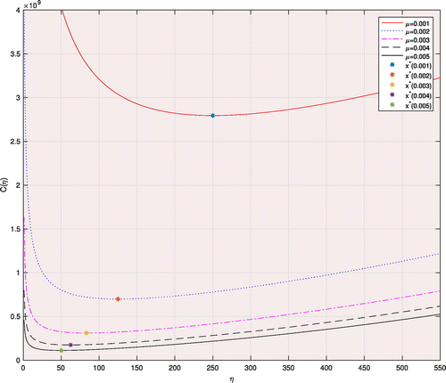
Lemma 3 allows for claiming that $\widehat{C}(\eta )$ has a unique minimizer ${\eta }^{*}$; in fact, such a minimizer can be computed by a standard semismooth Newton method (Facchinei and Pang 2003). Figure 1 provides a schematic of $\widehat{C}(\eta )$ for different values of μ, whereas ${\eta }^{*}$ is computed by semismooth Newton method. We note that, when μ is larger, ${\eta }^{*}(\mu )$ tends to be smaller. In such cases, obtaining an optimal ${\eta }^{*}$ is particularly useful. However, when $\mu \ll 1$, we observe that ${\eta }^{*}(\mu )\gg 1$; consequently, this leads to rescaling of the step γ_k to $\frac{{\gamma }_k}{\eta }$, resulting in poorer behavior. Therefore, if $\mu \ll 1$, we employ η = 1, and this has far better empirical behavior as seen in the numerics.

2.4. Linear Convergence of mVS-PM: Non-compact Domains

In this section, we derive rate and complexity guarantees when (VS-PM), an unaccelerated variant of VS-APM, is applied on a Moreau-smoothed problem under possibly noncompact domains and under a (weaker) state-dependent bound on the subgradient (Assumption 5). When the subgradient of g is characterized by a state-dependent bound, the bound on the cumulative error in the accelerated method builds up because of a recursive relation, see (A.16). Hence, in this section, we consider a more general case in which Assumption 5 imposes a state-dependent bound, weakening Assumption 4. By employing an unaccelerated method, we derive a similar oracle complexity as in Section 2.3. To obtain rate results, we apply (VS-PM) with the following update rule:

where ${\nabla }_x{F}_{\eta }(x_k)+{\overline{w}}_{k,N_k}$ can be obtained by solving ${\min }_{u\in {\mathbb{R}}^n}[\mathbb{E}[\tilde{F}(u,\omega )]+\frac{1}{2\eta }\Vert u-x_k{\Vert }^2]$ inexactly taking N_k (stochastic) subgradient steps. Consider the sequence of iterates $\{x_k\}$ generated by applying an inexact gradient scheme on the following strongly convex smooth optimization problem.

In effect, given an $x_0\in {\mathbb{R}}^n$, the inexact gradient scheme generates a sequence $\{x_k\}$ such that

Given an x_k, we denote the update with the exact gradient by ${\overline{x}}_{k+1}$, which is defined as follows.

Recall that ${\nabla }_x{F}_{\eta }(x_k)$ is defined as ${\nabla }_x{F}_{\eta }(x_k)=\frac{1}{\eta }(x_k-z_k^{*})$, where $z_k^{*}$ is the unique minimizer of the following problem, that is,

In other words, $z_k^{*}$ is defined as

Because ${\text{prox}}_{\eta F}(x_k)$ is unavailable in closed form, we may compute increasingly exact analogs; given $z_{k,0}=x_k$, we construct the sequence ${\{z_{k,j}\}}_{j=1}^{N_k}$ based on (SSG).

Consequently, at major iteration k, the inexact gradient of $F_{\eta }(x)$ is given by $\frac{1}{\eta }(x_k-z_{k,N_k})$, implying that ${\overline{w}}_k$ is defined as $\frac{1}{\eta }(z_k^{*}-z_{k,N_k}).$ Consequently, we have that

We proceed to derive a bound on the conditional second moment of $G(z_{k,j},{\omega }_{k,j})=S(z_{k,j},{\omega }_{k,j})+\frac{1}{\eta }(z_{k,j}-x_k)$, where $S(z_{k,j},{\omega }_{k,j})\in \partial \tilde{F}(z_{k,j},{\omega }_{k,j}),\hspace{0.17em}{M}_1^2\triangleq 2{\overline{M}}^2+\frac{4}{{\eta }^2},\hspace{0.17em}{M}_2^2\triangleq \frac{4}{{\eta }^2}$, and $M_3^2\triangleq 2M^2$. This requires defining the history up to iteration j at outer iteration k by ${\mathcal{F}}_{k,j}$ as follows.

We now outline an assumption on the bound on the stochastic subgradient that scales with the size of x allowing for noncompact domains.

Assumption 5.

Let $\{x_k\}$ be a sequence generated by (VS-PM), where ${\nabla }_x{F}_{\eta }(x_k)+{\overline{w}}_{k,N_k}$ is computed by taking N_k steps of (SSG), leading to a set of iterates $\{z_{k,1},\cdots ,z_{k,N_k}\}$. Let ${\mathcal{F}}_{k,j}$ be defined as (19) for $k\ge 1$ and $j=1,\cdots ,N_k$. For any $z_{k,j}$, let $S(z_{k,j},{\omega }_{k,j})$ denote a measurable selection $S(z_{k,j},{\omega }_{k,j})\in \partial \tilde{F}(z_{k,j},{\omega }_{k,j})$. With these constructs, the following are assumed to hold.

1. Unbiasedness: we have that $\mathbb{E}[S(z_{k,j},{\omega }_{k,j})|{\mathcal{F}}_{k,j}]=S(z_{k,j})\in \partial F(z_{k,j})$ almost surely.

2. Subgradient boundedness: there exists $M,\overline{M}>0$ such that, for any x, $\mathbb{E}[\Vert S(z_{k,j},{\omega }_{k,j}){\Vert }^2|{\mathcal{F}}_{k,j}]\le {\overline{M}}^2\Vert z_{k,j}{\Vert }^2+M^2$ almost surely.

Consequently, we have that

Based on Assumption 5 and inspired by a proof technique from Chambolle and Pock (2011) among others, we derive a rate statement for (SSG) (see appendix for proof).

Proposition 1.

Consider (17) in which $F(·,\omega )$ is a μ-strongly convex function and $S(z,\omega )\in \partial \tilde{F}(z,\omega )$ for any z. Suppose Assumption 5 holds and ${\widehat{a}}^2\triangleq 4+4M_1^2+2M_2^2$ and ${\widehat{b}}^2\triangleq (4M_1^2+2M_2^2)[\Vert x^{*}{\Vert }^2]+M_3^2.$ Given x_k, consider a sequence generated by (SSG) in which $\tilde{\mu }=\mu +\frac{1}{\eta }$, $\overline{J}\triangleq \lceil \frac{2M_1^2}{{\tilde{\mu }}^2}-1\rceil$, and

$${\sigma }_j\triangleq \{\begin{array}{ll}\min \left\{\frac{1}{(j+1)\log (j+1)},\frac{\tilde{\mu }}{M_1^2}\right\},\hfill & j<\overline{J}\hfill \\ \frac{1}{(j+1)\log (j+1)}.\hfill & j\ge \overline{J}\hfill \end{array}$$

Then, the following holds for $j\ge \overline{J}$.

$$\mathbb{E}[\Vert z_{k,j}-z_k^{*}{\Vert }^2\hspace{0.17em}|{\mathcal{F}}_k]\le \frac{{\widehat{a}}^2\Vert x_k-x^{*}{\Vert }^2+{\widehat{b}}^2}{j}.$$(21)

We now show the convergence of mVS-PM when ${\nabla }_x{F}_{\eta }(x)$ is approximated via (SSG) (see appendix for proof).

Theorem 3

(mVS-PM Under State-Dependent Bound on Subgradients). Suppose Assumptions 1 and 5 hold. Consider the iterates generated by (VS-PM) applied on $F_{\eta }(x)$, where $\tilde{\kappa }\triangleq 1+\frac{1}{\eta \mu },\hspace{0.17em}\gamma =\eta$ and $N_k\triangleq \lfloor N_0{\rho }^{-k}\rfloor$ for all $k\ge 0$, $N_0>\max \left\{\frac{2{\widehat{a}}^2}{(1-q/2)},\overline{J}\right\}$, $q\triangleq 1-\frac{1}{\tilde{\kappa }}$, $p_0\triangleq \frac{q}{2}+\frac{2{\widehat{a}}^2}{N_0}$, and $\overline{J}\triangleq \lceil \frac{2M_1^2}{{\overline{\mu }}^2}-1\rceil$. Then, the following hold.

1. Rate: for all $k\ge 1$, we have that the following holds.

   $$\mathbb{E}[\Vert x_k-x^{*}{\Vert }^2]\le \mathcal{C}{\widehat{p}}^k \mathit{where} \mathcal{C}\triangleq \left(\mathbb{E}[\Vert x_0-x^{*}{\Vert }^2]+\frac{\widehat{b}\widehat{D}}{N_0}\right),\{\begin{array}{ll}\rho \ne p_0,\hfill & \widehat{p}=\max \{\rho ,p_0\},\widehat{D}\triangleq \frac{1}{1-\frac{\min \{\rho ,p_0\}}{\max \{\rho ,p_0\}}}\hfill \\ \rho =p_0.\hfill & \widehat{p}\in (p_0,1),\widehat{D}>\frac{1}{\ln {(p_0/\widehat{p})}^e}\hfill \end{array}$$

2. Iteration complexity: the iteration complexity of mVS-PM in gradient steps of (${\nabla }_x{F}_{\eta }(x_k))$ to obtain an ϵ-accurate solution is $\mathcal{O}(\tilde{\kappa }\log (\mathcal{C}/ϵ))$.

3. Oracle complexity in (SSG) steps: to compute x_K such that $\mathbb{E}[\Vert x_K-x^{*}{\Vert }^2]\le ϵ$, the complexity in subgradient steps is bounded as ${\sum }_{k=1}^K{N}_k\le \mathcal{O}\left(\tilde{\kappa }{\left(\frac{\mathcal{C}}{ϵ}\right)}^{{\log }_{1/\widehat{p}}(1/\rho )}\right)$ for $\widehat{p}\in [p_0,1),\hspace{0.17em}\rho \le p_0$ and ${\sum }_{k=1}^K{N}_k\le \mathcal{O}\left(\tilde{\kappa }\left(\frac{\mathcal{C}}{ϵ}\right)\right)$ for $\rho >p_0$.

Remark 3.

We observe that, when $\rho >p_0$, we achieve the optimal oracle complexity in subgradient steps akin to the statement in the regime of bounded subgradients. Notably, $\tilde{\kappa }$ can be controlled because η is any nonnegative scalar. For instance, if $\eta =\frac{1}{\mu }$, $\tilde{\kappa }=2$.

3. Iteratively Smoothed VS-APM for Nonsmooth Convex Problems

Thus far, we consider settings in which f is a strongly convex function. However, there are many instances when the function f is neither smooth nor strongly convex. In fact, in strongly convex regimes, estimating the strong convexity parameter may often be challenging. In such settings, if the function f is subdifferentiable, then subgradient methods provide an avenue for resolving such problems in stochastic regimes but display a significantly poorer rate of convergence. Nesterov (2005b) shows that, for a subclass of problems, an accelerated gradient scheme may be applied to a suitably smoothed problem in which the smoothing leads to a differentiable problem with Lipschitz continuous gradients (with known Lipschitz constants). If the smoothing parameter is chosen suitably, the convergence rate to an approximate solution can be improved to $\mathcal{O}(1/K)$ from $\mathcal{O}(1/\sqrt{K})$ in terms of expected suboptimality. However, because the smoothing parameter is maintained as fixed, Nesterov’s approach can provide approximate solutions at best but not asymptotically exact solutions. Subsequently, Nesterov (2005a) considers a primal–dual smoothing technique in which the smoothing parameter is reduced at every step, whereas extensions and generalizations are considered more recently by Tran-Dinh et al. (2018) and Van Nguyen et al. (2017). In this section, we develop an iteratively smoothed, variable sample-size, accelerated proximal gradient scheme that can contend with expectation-valued objectives and is asymptotically convergent. This can be viewed as a variant of the primal smoothing scheme introduced by Nesterov (2005b), in which the smoothing parameter is reduced after every step; this scheme is shown to admit a rate of $\mathcal{O}(1/K)$, matching the finding by Nesterov (2005b); however, our scheme is blessed with asymptotic guarantees rather than providing approximate solutions. In Section 3.1, we derive rate and complexity statements, in Section 3.2 for the iteratively smoothed VS-APM (or sVS-APM), recovering the optimal rate of $\mathcal{O}(1/K^2)$ with the optimal oracle complexity of $\mathcal{O}(1/{ϵ}^2)$ under smoothness. Finally, in Section 3.3, under suitable choices of smoothing sequences, sVS-APM produces sequences that converge a.s. to an optimal solution.

3.1. Smoothing Techniques

In this section, we consider minimizing F where F is defined as $F(x)\triangleq \mathbb{E}[\tilde{F}(x,\omega )]$, where $\tilde{f}(x,\omega )=\tilde{f}(x,\omega )+g(x)$ such that $f$ and $g$ are convex and may be nonsmooth, whereas g has an efficient prox evaluation (or “proximable”) but f is not proximable. Note that this setting is more general than structured nonsmooth problems, in which the function $f$ is considered to be convex and smooth. In contrast to the previous section, we assume that ${\nabla }_x{\tilde{f}}_{{\eta }_k}(x_k,{\omega }_k)$ is generated from the stochastic oracle, in which η_k is a smoothing parameter at iteration k such that its sequence is diminishing. Beck and Teboulle (2012) define an $(\alpha ,\beta )$-smoothable function as follows.

Definition 1

($(\alpha ,\beta )$-Smoothable; Beck 2017). A convex function $h:{\mathbb{R}}^n\to \mathbb{R}$ is referred to as $(\alpha ,\beta )$-smoothable if, for any $\eta >0$, there exists a convex differentiable function $h_{\eta }:{\mathbb{R}}^n\to \mathbb{R}$ that satisfies the following: (i) $h_{\eta }(x)\le h(x)\le h_{\eta }(x)+\eta \beta$ for all x, and (ii) $h_{\eta }$ is $\alpha /\eta$ smooth.

There are a host of smoothing functions based on the nature of $h$. For instance, when $h(x)=\Vert x|{|}_2$, then $h_{\eta }(x)=\sqrt{\Vert x{\Vert }_2^2+{\eta }^2}-\eta$, implying that $h$ is a (1, 1)-smoothable function. If $h(x)=\max \{x_1,x_2, \dots ,x_n\}$, then $h$ is $(1,\log (n))$-smoothable and $h_{\eta }(x)=\eta \log ({\sum }_{i=1}^n{e}^{x_i/\eta })-\eta \log (n).$ (see Beck and Teboulle 2012 for more examples). Recall that, when $h$ is a proper, closed, and convex function, the Moreau envelope is defined as $h_{\eta }(x)\triangleq {\min }_u\hspace{0.17em}\{h(u)+\frac{1}{2\eta }\Vert u-x{\Vert }^2\}.$ In fact, $h$ is $(1,B^2)$-smoothable when $h_{\eta }$ is given by the Moreau envelope (see Beck and Teboulle 2012) and B denotes a uniform bound on $\Vert s\Vert$ in x, where $s\in \partial h(x)$. There are a range of other smoothing techniques, including Nesterov smoothing (see Nesterov 2005b) and inf-conv smoothing (see Beck 2017); our approach is agnostic to the choice of smoothing. In particular, if $\tilde{f}(·,\omega )$ is a proper, closed, and convex function in x for every ω, then $\tilde{f}(·,\omega )$ is $(1,B^2)$-smoothable for every ω for which ${\tilde{f}}_{\eta }(·,\omega )$ is a suitable smoothing. In fact, if $\tilde{f}(·,\omega )$ satisfies the following smoothability assumption, then smoothability of f follows as shown by Lemma 4. It is worth emphasizing that the smoothing of f, denoted by $f_{\eta }$, is defined as

$$f_{\eta }(x)\triangleq \mathbb{E}[{\tilde{f}}_{\eta }(x,\omega )],$$(22)

where ${\tilde{f}}_{\eta }(·,\omega )$ is a smoothing of $\tilde{f}(·,\omega )$.

Assumption 6.

The function $\tilde{f}(·,\omega )$ is an $(\alpha (\omega ),\beta (\omega ))$-smoothable function for every $\omega \in \mathrm{\Omega }$, where $\mathbb{E}[\alpha (\omega )]\le \tilde{\alpha }$ and $\mathbb{E}[\beta (\omega )]\le \tilde{\beta }$ with $\tilde{\alpha },\tilde{\beta }>0;$ that is, for any $\eta >0$, there exists a convex differentiable function ${\tilde{f}}_{\eta }(·,\omega )$ for every $\omega \in \mathrm{\Omega }$ such that

$$\begin{array}{l}{\tilde{f}}_{\eta }(x,\omega )\le \tilde{f}(x,\omega )\le {\tilde{f}}_{\eta }(x,\omega )+\eta \beta (\omega ),\hspace{1em} \mathit{for} \mathit{all} x\hfill \\ \mathit{\text{and}} \Vert {\nabla }_x{\tilde{f}}_{\eta }(x,\omega )\text{-}{\nabla }_x{\tilde{f}}_{\eta }(y,\omega )\Vert \le \frac{\alpha (\omega )}{\eta }\Vert x-y\Vert ,\hspace{1em}\hspace{1em}\hspace{1em} \mathit{for} \mathit{all} \hspace{0.17em}x,y,\hfill \end{array}$$

where $\mathbb{E}[\alpha (\omega )]\le \tilde{\alpha }$ and $\mathbb{E}[\beta (\omega )]\le \tilde{\beta }$.

Based on the following lemma, we observe that f is $(\tilde{\alpha },\tilde{\beta })$-smoothable if $\tilde{f}(·,\omega )$ satisfies suitable smoothability requirements for almost every $\omega \in \mathrm{\Omega }$.

Lemma 4.

Suppose Assumption 6 holds. Then, there exist $\tilde{\alpha },\tilde{\beta }>0$ such that f is $(\tilde{\alpha },\tilde{\beta })$-smoothable, where $f(x)\triangleq \mathbb{E}[\tilde{f}(x,\omega )]$.

We proceed to develop a smoothed variant of VS-APM, referred to as sVS-APM, in which ${\nabla }_x{\tilde{f}}_{{\eta }_k}(x_k,{\omega }_k)$ is generated from the stochastic oracle and η_k is driven to zero at a sufficient rate (See Algorithm 2).

Algorithm 2

(Iteratively Smoothed VS-APM (sVS-APM))

• (0) Given budget M, $x_0\in X$, y₀ = x₀ and positive sequences $\{{\gamma }_k,N_k\}$. Set ${\lambda }_0=0,\hspace{0.17em}{\lambda }_1=1$; $k≔1$.

• (1) $y_{k+1}={\mathbf{P}}_{{\gamma }_k,g}(x_k-{\gamma }_k({\nabla }_x{f}_{{\eta }_k}(x_k)+{\overline{w}}_{k,N_k}))$;

• (2) ${\lambda }_{k+1}=\frac{1+\sqrt{1+4{\lambda }_k^2}}{2}$;

• (3) $x_{k+1}=y_{k+1}+\frac{({\lambda }_k-1)}{{\lambda }_{k+1}}(y_{k+1}-y_k)$;

• (4) If ${\sum }_{j=1}^k{N}_j>M$, then stop; else $k≔k+1$; return to (1).

3.2. Rate and Complexity Analysis

In this section, we develop rate and oracle complexity statements for Algorithm 2 when f is $(1,B^2)$ smoothable and then specialize these results to both the deterministic nonsmooth and stochastic smooth regimes. We begin with a modified assumption.

Assumption 7.

(i) The function g is lower semicontinuous and convex with effective domain denoted by $\text{dom}(g)$; (ii) f is proper, closed, convex, and $(1,B^2)$-smoothable on an open set containing $\text{dom}(g)$; (iii) there exists C > 0 such that $\mathbb{E}[\Vert x_0-x^{\ast }\Vert ]\le C$ for all $x^{*}\in X^{*}$.

Note that Assumption 6 represents a set of sufficiency conditions for f to be smoothable; here, we directly assume that f is smoothable to ease exposition.

Lemma 5.

Suppose Assumption 7 holds. Consider the iterates generated by sVS-APM on F(x). Suppose Assumption 3 holds for $f_{{\eta }_k}(x)$. If $\{{\gamma }_k\}$ is a decreasing sequence and ${\gamma }_k\le {\eta }_k/2$, then the following holds for all $K\ge 2$:

$$\mathbb{E}[F_{{\eta }_k}(y_K)-F_{{\eta }_k}(x^{*})]\le \frac{2}{{\gamma }_{K-1}{(K-1)}^2}{\displaystyle \sum _{k=1}^{K-1}{\gamma }_k^2}{k}^2\frac{{\nu }^2}{N_k}+\frac{2C^2}{{\gamma }_{K-1}{(K-1)}^2}.$$

Proof.

By the update rule in Algorithm 2, we have

$$y_{k+1}=\arg \underset{x}{\min }\hspace{0.17em}g(x)+\frac{1}{2{\gamma }_k}\Vert x-x_k{\Vert }^2+{({\nabla }_x{f}_{{\eta }_k}(x_k)+{\overline{w}}_k)}^{T}x.$$(23)

From the optimality condition for (23), $0\in \partial g(y_{k+1})+\frac{1}{{\gamma }_k}(y_{k+1}-x_k)+{\nabla }_x{f}_{{\eta }_k}(x)+{\overline{w}}_k$. By convexity of g(x), we have that $g(x)\ge g(y_k)+s^T(x-y_{k+1})$ for all $s\in \partial g(y_k)$. Hence, we obtain the following.

$$g(x)+{({\nabla }_x{f}_{{\eta }_k}(x_k)+{\overline{w}}_k)}^{T}x\ge g(y_{k+1})+{({\nabla }_x{f}_{{\eta }_k}(x_k)+{\overline{w}}_k)}^T{y}_{k+1}-\frac{1}{{\gamma }_k}{(x-y_{k+1})}^T(y_{k+1}-x_k).$$

Now, by using Lemma A.2, we obtain that

$$\begin{array}{ll}\hfill & \hspace{1em}\hspace{1em}g(x)+{({\nabla }_x{f}_{{\eta }_k}(x_k)+{\overline{w}}_k)}^{T}x+\frac{1}{2{\gamma }_k}\Vert x-x_k{\Vert }^2\hfill \\ \hfill & \ge g(y_{k+1})+{({\nabla }_x{f}_{{\eta }_k}(x_k)+{\overline{w}}_k)}^T{y}_{k+1}+\frac{1}{2{\gamma }_k}\Vert x_k-y_{k+1}{\Vert }^2+\frac{1}{2{\gamma }_k}\Vert x-y_{k+1}{\Vert }^2.\hfill \end{array}$$(24)

By invoking the convexity of $f_{{\eta }_k}$ and by using the Lipschitz continuity of ${\nabla }_x{f}_{{\eta }_k}$, we obtain

$$\begin{array}{ll}{f}_{{\eta }_k}(x)\hfill & \ge f_{{\eta }_k}(x_k)+{\nabla }_x{f}_{{\eta }_k}{(x_k)}^T(x-x_k)\hfill \\ \hfill & \ge f_{{\eta }_k}(y_{k+1})+{\nabla }_x{f}_{{\eta }_k}{(x_k)}^T(x-y_{k+1})-\frac{1}{2{\eta }_k}\Vert x_k-y_{k+1}{\Vert }^2\hfill \\ \hfill & =f_{{\eta }_k}(y_{k+1})+{({\nabla }_x{f}_{{\eta }_k}(x_k)+{\overline{w}}_k)}^T(x-y_{k+1})-\frac{1}{2{\eta }_k}\Vert x_k-y_{k+1}{\Vert }^2-{\overline{w}}_k^T(x-y_{k+1}),\hfill \end{array}$$(25)

where the last equality follows from adding and subtracting ${\overline{w}}_k$. By adding (24) and (25), we obtain

$$\begin{array}{ll}{F}_{{\eta }_k}(y_{k+1})-F_{{\eta }_k}(x)\hfill & \le \frac{1}{2{\gamma }_k}\Vert x-x_k{\Vert }^2-\frac{1}{2{\gamma }_k}\Vert x-y_{k+1}{\Vert }^2+\frac{1}{2}\left(\frac{1}{{\eta }_k}-\frac{1}{{\gamma }_k}\right)\Vert x_k-y_{k+1}{\Vert }^2-{\overline{w}}_k^T(y_{k+1}-x)\hfill \\ \hfill & =\left(\frac{1}{2{\eta }_k}-\frac{1}{{\gamma }_k}\right)\Vert x_k-y_{k+1}{\Vert }^2+\frac{1}{{\gamma }_k}{(x_k-y_{k+1})}^T(x_k-x)-{\overline{w}}_k^T(y_{k+1}-x),\hfill \end{array}$$(26)

where the last inequality follows from Lemma A.2 by choosing Q = I, $v_1=x_k,\hspace{0.17em}{v}_2=x$, and $v_3=y_k$. By setting $x=y_k$ in (26), we have

$$\begin{array}{ll}{F}_{{\eta }_k}(y_{k+1})-F_{{\eta }_k}(y_k)\hfill & \le \left(\frac{1}{2{\eta }_k}-\frac{1}{{\gamma }_k}\right)\Vert x_k-y_{k+1}{\Vert }^2+\frac{1}{{\gamma }_k}{(x_k-y_{k+1})}^T(x_k-y_k)\hfill \\ \hfill & -{\overline{w}}_{k,N_k}^T(y_{k+1}-y_k).\hfill \end{array}$$(27)

Similarly, by letting $x=x^{*}$, we can obtain

$$\begin{array}{ll}{F}_{{\eta }_k}(y_{k+1})-F_{{\eta }_k}(x^{*})\hfill & \le \left(\frac{1}{2{\eta }_k}-\frac{1}{{\gamma }_k}\right)\Vert x_k-y_{k+1}{\Vert }^2+\frac{1}{{\gamma }_k}{(x_k-y_{k+1})}^T(x_k-x^{*})\hfill \\ \hfill & -{\overline{w}}_{k,N_k}^T(y_{k+1}-x^{*}).\hfill \end{array}$$(28)

By invoking Lemma A.2 in which $v_1=x_k,\hspace{0.17em}{v}_2=y_{k+1}$ and $v_3=y_k$, we obtain

$$\frac{1}{{\gamma }_k}{(y_{k+1}-x_k)}^T(y_k-x_k)=\frac{1}{2{\gamma }_k}(\Vert y_k-x_k{\Vert }^2+\Vert y_{k+1}-x_k{\Vert }^2-\Vert y_{k+1}-y_k{\Vert }^2).$$

Consequently, (27) can further bounded as follows:

$$\begin{array}{ll}\hfill & F_{{\eta }_k}(y_{k+1})-F_{{\eta }_k}(y_k)\le \left(\frac{1}{2{\eta }_k}-\frac{1}{{\gamma }_k}\right)\Vert x_k-y_{k+1}{\Vert }^2+\frac{1}{{\gamma }_k}{(x_k-y_{k+1})}^T(x_k-y_k)-{\overline{w}}_{k,N_k}^T(y_{k+1}-y_k)\hfill \\ \hfill & =\left(\frac{1}{2{\eta }_k}-\frac{1}{{\gamma }_k}\right)\Vert x_k-y_{k+1}{\Vert }^2+\frac{1}{2{\gamma }_k}(\Vert x_k-y_k{\Vert }^2+\Vert y_{k+1}-x_k{\Vert }^2-\Vert y_{k+1}-y_k{\Vert }^2)-{\overline{w}}_{k,N_k}^T(y_{k+1}-y_k)\hfill \\ \hfill & =\left(\frac{1}{2{\eta }_k}-\frac{1}{2{\gamma }_k}\right)\Vert x_k-y_{k+1}{\Vert }^2+\frac{1}{2{\gamma }_k}(\Vert x_k-y_k{\Vert }^2-\Vert y_{k+1}-y_k{\Vert }^2)-{\overline{w}}_{k,N_k}^T(y_{k+1}-y_k).\hfill \end{array}$$(29)

Similarly, we have that

$$\begin{array}{ll}{F}_{{\eta }_k}(y_{k+1})-F_{{\eta }_k}(x^{*})\hfill & \le \left(\frac{1}{2{\eta }_k}-\frac{1}{2{\gamma }_k}\right)\Vert x_k-y_{k+1}{\Vert }^2+\frac{1}{2{\gamma }_k}(\Vert x_k-x^{*}{\Vert }^2-\Vert y_{k+1}-x^{*}{\Vert }^2)\hfill \\ \hfill & -{\overline{w}}_{k,N_k}^T(y_{k+1}-x^{*}).\hfill \end{array}$$(30)

By multiplying (29) by $({\lambda }_k-1)$ and adding to (30), where ${\delta }_k\triangleq F_{{\eta }_k}(y_k)-F_{{\eta }_k}(x^{*})$, we have

$${\lambda }_k{\delta }_{k+1}-({\lambda }_k-1){\delta }_k\le \left(\frac{1}{2{\eta }_k}-\frac{1}{2{\gamma }_k}\right){\lambda }_k\Vert y_{k+1}-x_k{\Vert }^2$$(31)

$$+\frac{1}{2{\gamma }_k}({\lambda }_k-1)(\Vert x_k-y_k{\Vert }^2-\Vert y_{k+1}-y_k{\Vert }^2)+\frac{1}{2{\gamma }_k}(\Vert x_k-x^{*}{\Vert }^2-\Vert y_{k+1}-x^{*}{\Vert }^2)$$(32)

$$+{\overline{w}}_{k,N_k}^T(({\lambda }_k-1)y_k+x^{*}-{\lambda }_k{y}_{k+1}).$$(33)

Again, by using Lemma A.2, we may express the terms in (32) as follows:

$$\begin{array}{ll}\hfill & \hspace{0.17em}\frac{1}{2{\gamma }_k}({\lambda }_k-1)(\Vert x_k-y_k{\Vert }^2-\Vert y_{k+1}-y_k{\Vert }^2)+\frac{1}{2{\gamma }_k}(\Vert x_k-x^{*}{\Vert }^2-\Vert y_{k+1}-x^{*}{\Vert }^2)\hfill \\ \hfill & =\frac{1}{2{\gamma }_k}({\lambda }_k\Vert x_k-y_k{\Vert }^2-{\lambda }_k\Vert y_{k+1}-y_k{\Vert }^2-\Vert x_k-y_k{\Vert }^2+\Vert y_{k+1}-y_k{\Vert }^2+\Vert x_k-x^{*}{\Vert }^2-\Vert y_{k+1}-x^{*}{\Vert }^2)\hfill \\ \hfill & =\frac{1}{2{\gamma }_k}(-{\lambda }_k\Vert y_{k+1}-x_k{\Vert }^2+2{\lambda }_k{(y_{k+1}-x_k)}^T(y_k-x_k)+\Vert y_{k+1}-x_k{\Vert }^2-2{(y_{k+1}-x_k)}^T(y_k-x_k)\hfill \\ \hfill & -\Vert y_{k+1}-x_k{\Vert }^2+2{(y_{k+1}-x_k)}^T(x^{*}-x_k))\hfill \\ \hfill & =\frac{1}{2{\gamma }_k}\left(-{\lambda }_k\Vert y_{k+1}-x_k{\Vert }^2+2{(y_{k+1}-x_k)}^T(({\lambda }_k-1)y_k-{\lambda }_k{x}_k+x^{*})\right).\hfill \end{array}$$

In addition,

$$\hspace{1em}{\overline{w}}_{k,N_k}^T(({\lambda }_k-1)y_k+x^{*}-{\lambda }_k{y}_{k+1})={\overline{w}}_{k,N_k}^T(({\lambda }_k-1)y_k+x^{*}-{\lambda }_k{x}_k)+{\overline{w}}_{k,N_k}^T({\lambda }_k{x}_k-{\lambda }_k{y}_{k+1}).$$

From the update rule, ${\lambda }_{k-1}^2={\lambda }_k({\lambda }_k-1)={\lambda }_k^2-{\lambda }_k$. Now, by multiplying (31) by λ_k, we obtain the following, in which $u_k=({\lambda }_k-1)y_k-{\lambda }_k{x}_k+x^{*}$:

$$\begin{array}{ll}\hfill & \hspace{1em}{\lambda }_k^2{\delta }_{k+1}-{\lambda }_{k-1}^2{\delta }_k\le {\lambda }_k^2\left(\frac{1}{2{\eta }_k}-\frac{1}{2{\gamma }_k}\right)\Vert y_{k+1}-x_k{\Vert }^2\hfill \\ \hfill & +\frac{1}{2{\gamma }_k}\left(-\Vert {\lambda }_k{y}_{k+1}-{\lambda }_k{x}_k{\Vert }^2+2{({\lambda }_k{y}_{k+1}-{\lambda }_k{x}_k)}^T(({\lambda }_k-1)y_k+x^{*}-{\lambda }_k{x}_k)\right)\hfill \\ \hfill & -{\lambda }_k^2{\overline{w}}_{k,N_k}^T(x_k-y_{k+1})-{\lambda }_k{w}_k^T{u}_k={\lambda }_k^2\left(\frac{1}{2{\eta }_k}-\frac{1}{2{\gamma }_k}\right)\Vert y_{k+1}-x_k{\Vert }^2-{\lambda }_k^2{\overline{w}}_{k,N_k}^T(x_k-y_{k+1})\hfill \\ \hfill & +\frac{1}{2{\gamma }_k}(\Vert {\lambda }_k{x}_k-({\lambda }_k-1)y_k-x^{*}{\Vert }^2-\Vert {\lambda }_k{y}_{k+1}-({\lambda }_k-1)y_k-x^{*}{\Vert }^2)-{\lambda }_k{w}_k^T{u}_k\hfill \\ \hfill & \le \frac{{\lambda }_k^2}{\frac{2}{{\gamma }_k}-\frac{2}{{\eta }_k}}\Vert {\overline{w}}_{k,N_k}{\Vert }^2+\frac{1}{2{\gamma }_k}(\Vert u_k{\Vert }^2-\Vert u_{k+1}{\Vert }^2)-{\lambda }_k{w}_k^T{u}_k,\hfill \end{array}$$(34)

where, in the last inequality, we use the update rule of algorithm, $x_{k+1}=y_{k+1}+\frac{{\lambda }_k-1}{{\lambda }_{k+1}}(y_{k+1}-y_k)$, to obtain the following:

$$u_{k+1}=({\lambda }_{k+1}-1)y_{k+1}-{\lambda }_{k+1}{x}_{k+1}+x^{*}=({\lambda }_k-1)y_k-{\lambda }_k{y}_{k+1}+x^{*}.$$

By multiplying both sides by γ_k and assuming ${\gamma }_k\le {\gamma }_{k-1}$, we obtain

$${\gamma }_k{\lambda }_k^2{\delta }_{k+1}-{\gamma }_{k-1}{\lambda }_{k-1}^2{\delta }_k\le \frac{{\gamma }_k{\lambda }_k^2}{\frac{2}{{\gamma }_k}-\frac{2}{{\eta }_k}}\Vert {\overline{w}}_{k,N_k}{\Vert }^2+\frac{1}{2}(\Vert u_k{\Vert }^2-\Vert u_{k+1}{\Vert }^2)-{\gamma }_k{\lambda }_k{w}_k^T{u}_k.$$(35)

By assuming ${\gamma }_k\le \frac{{\eta }_k}{2}$, we obtain $\frac{1}{{\gamma }_k}-\frac{1}{{\eta }_k}\ge \frac{1}{2{\gamma }_k}$, implying that

$${\gamma }_k{\lambda }_k^2{\delta }_{k+1}-{\gamma }_{k-1}{\lambda }_{k-1}^2{\delta }_k\le {\gamma }_k^2{\lambda }_k^2\Vert {\overline{w}}_{k,N_k}{\Vert }^2+\frac{1}{2}(\Vert u_k{\Vert }^2-\Vert u_{k+1}{\Vert }^2)-{\gamma }_k{\lambda }_k{w}_k^T{u}_k.$$(36)

Summing (36) from k = 1 to K – 1, we have the following:

$$\begin{array}{ll}\hfill & {\gamma }_{K-1}{\lambda }_{K-1}^2{\delta }_K\le {\displaystyle \sum _{k=1}^{K-1}{\gamma }_k^2}{\lambda }_k^2\Vert {\overline{w}}_{k,N_k}{\Vert }^2+\frac{1}{2}\Vert u_1{\Vert }^2-{\displaystyle \sum _{k=1}^{K-1}{\gamma }_k}{\lambda }_k{w}_k^T{u}_k\hfill \\ \hfill & \Rightarrow {\delta }_K\le \frac{1}{{\gamma }_{K-1}{\lambda }_{K-1}^2}{\displaystyle \sum _{k=1}^{K-1}{\gamma }_k^2}{\lambda }_k^2\Vert {\overline{w}}_{k,N_k}{\Vert }^2+\frac{1}{2{\gamma }_{K-1}{\lambda }_{K-1}^2}\Vert u_1{\Vert }^2-\frac{1}{{\gamma }_{K-1}{\lambda }_{K-1}^2}{\displaystyle \sum _{k=1}^{K-1}{\gamma }_k}{\lambda }_k{w}_k^T{u}_k.\hfill \end{array}$$

Taking expectations, we note that the last term on the right is zero (under a zero-bias assumption), leading to the following:

$$\begin{array}{ll}\mathbb{E}[{\delta }_K]\le \frac{1}{{\gamma }_{K-1}{\lambda }_{K-1}^2}{\displaystyle \sum _{k=1}^{K-1}{\gamma }_k^2}{\lambda }_k^2\frac{{\nu }^2}{N_k}+\frac{1}{2{\gamma }_{K-1}{\lambda }_{K-1}^2}\mathbb{E}[\Vert u_1{\Vert }^2\Vert ]\hfill & \le \frac{2}{{\gamma }_{K-1}{(K-1)}^2}{\displaystyle \sum _{k=1}^{K-1}{\gamma }_k^2}{k}^2\frac{{\nu }^2}{N_k}\hfill \\ \hfill & +\frac{2C^2}{{\gamma }_{K-1}{(K-1)}^2},\hfill \end{array}$$

where, in the last inequality, we use the fact that $\Vert y-x^{*}\Vert \le C$ for all $y\in \text{dom}(g)$ and $\frac{k}{2}\le {\lambda }_k\le k$, which may be shown inductively. □

We are now ready to prove our main rate result and oracle complexity bound for sVS-APM.

Theorem 4

(Rate Statement and Oracle Complexity Bound for sVS-APM). Suppose Assumption 7 holds. Consider the iterates generated by sVS-APM on F(x). Suppose Assumption 3 holds for $f_{{\eta }_k}$. Suppose $\{{\lambda }_k\}$ is specified in sVS-APM, ${\eta }_k=1/k,\hspace{0.17em}{\gamma }_k=1/2k$, and $N_k=\lfloor k^a\rfloor$.

1. The following holds for any $K\ge 1$:

   $$\mathbb{E}[F(y_{K+1})-F(x^{*})]\le \{\begin{array}{ll}\frac{\left(\frac{2{\nu }^{2}a}{a-1}+4C^2+B^2\right)}{K},\hfill & a=1+\delta ,\delta \in [{\delta }_L,{\delta }_U]\hfill \\ \frac{2{\nu }^2(1+\log (K))+4C^2+B^2}{K},\hfill & a=1\hfill \end{array}$$

2. Let $ϵ\le \tilde{C}/2$, and K is such that $\mathbb{E}[F(y_{K+1})-F(x^{*})]\le ϵ$. Then, the following holds.

   $${\displaystyle \sum _{k=1}^K{N}_k}\le \{\begin{array}{ll}\mathcal{O}\left(\frac{1}{{ϵ}^{2+{\delta }_L}}\right),\hfill & a=1+\delta ,\delta \in [{\delta }_L,{\delta }_U]\hfill \\ \mathcal{O}\left(\frac{1}{{ϵ}^2}{\log }^2(1/ϵ)\right).\hfill & a=1\hfill \end{array}$$

Proof.

• (i) If $N_k=\lfloor k^a\rfloor \ge \frac{1}{2}{k}^a$ and ${\gamma }_k=1/(2k)$ is utilized in Lemma 5, we obtain the following:

  $$\mathbb{E}[{\delta }_{K+1}]\le \frac{2{\nu }^2}{K}{\displaystyle \sum _{k=1}^K\frac{1}{k^a}}+\frac{4C^2}{K}.$$(37)

  1. $a=1+\delta$, where $\delta \in [{\delta }_L,{\delta }_U]$. Consequently, we may derive the next bound.

     $${\displaystyle \sum _{k=1}^K{k}^{-a}}=1+{\displaystyle \sum _{k=2}^K{k}^{-a}}\le 1+{\displaystyle {\int }_1^K{k}^{-a}}dk=1+\frac{1-K^{1-a}}{a-1}\le \frac{1+{\delta }_U}{{\delta }_L}.$$

     By invoking $(1,B^2)$-smoothability of f and ${\eta }_K=1/K$, we have that $F_{{\eta }_K}(y_{K+1})\le F(y_{K+1})$ and $-F_{{\eta }_K}(x^{*})\le -F(x^{*})+\eta B^2$. Hence, the required bound follows from (37)

     $$\mathbb{E}[F(y_{K+1})-F(x^{*})]\le \frac{2{\nu }^{2}a}{(a-1)K}+\frac{4C^2+B^2}{K}\le \frac{\overline{C}}{K}, \hspace{0.17em}\hspace{0.17em}\text{where} \overline{C}\triangleq \frac{2{\nu }^{2}a}{(a-1)}+4C^2+B^2.$$

  2. a = 1. Recall that the convergence rate is given by the following:

     $$\mathbb{E}[F(y_{K+1})-F(x^{*})]\le \frac{\frac{2{\nu }^2(a-K^{1-a})}{(a-1)}+4C^2+B^2}{K}.$$

  Taking limits, we obtain that

  $$\underset{a\to 1}{\lim }\frac{a-K^{1-a}}{a-1}=\underset{a\to 1}{\lim }\frac{1+K^{1-a}\log (K)}{1}=1+\log (K).$$

  Therefore, we have that

  $$\mathbb{E}[F(y_{K+1})-F(x^{*})]\le \frac{2{\nu }^2\log (K)+4C^2+B^2}{K}\triangleq \frac{a+b\log (K)}{K}.$$

• (ii) Consider $y_{K+1}$ satisfying $\mathbb{E}[F(y_{K+1})-F(x^{*})]\le ϵ$. We again consider two cases. a. $a=1+\delta$, where $\delta \in [{\delta }_L,{\delta }_U]$. We have $\frac{\overline{C}}{K}\le ϵ$, which implies that $K=\lceil \overline{C}/ϵ\rceil$. To obtain the optimal oracle complexity, we require ${\sum }_{k=1}^K{N}_k$ gradients. Hence, the following holds for sufficiently small ϵ such that $2\le \overline{C}/ϵ$:

  $${\displaystyle \sum _{k=1}^K{N}_k}\le {\displaystyle \sum _{k=1}^K{k}^a}={\displaystyle \sum _{k=1}^{1+\overline{C}/ϵ}{k}^a}\le {\displaystyle {\int }_0^{2+\overline{C}/ϵ}{k}^a}da=\frac{{(2+\overline{C}/ϵ)}^{1+a}}{1+a}\le {\left(\frac{\overline{C}}{ϵ}\right)}^{1+a}\le \mathcal{O}\left(\frac{1}{{ϵ}^{1+a}}\right)\le \mathcal{O}\left(\frac{1}{{ϵ}^{2+{\delta }_L}}\right).$$

b. a = 1. To compute K such that $\frac{a+b\log (K)}{K}\le ϵ$ is not immediately obvious but may be obtained via the Lambert function² (Chatzigeorgiou 2013). For purposes of simplicity, suppose a = 0 and b = 1. Then, we have the following.

$$\begin{array}{ll}\frac{\log (K)}{K}\le ϵ\hfill & \iff \frac{-\log (K)}{K}\ge -ϵ\hfill \\ \hfill & \iff W_{-1}\left(\frac{-\log (K)}{K}\right)\le W_{-1}(-ϵ), \hspace{0.17em}\hspace{0.17em}\text{since} W_{-1}(·) \hspace{0.17em}\hspace{0.17em}\text{is} \text{decreasing}.\hfill \end{array}$$

But $W_{-1}(-\frac{\log (x)}{x})=-\log (x)$ for x > e. Consequently, we have that

$$-\log (K)\le W_{-1}(-ϵ)\iff K\ge e^{-W_{-1}(-ϵ)}.$$

By definition of the Lambert function, we have that $e^{W(x)}=\frac{x}{W(x)}$, implying that

$$K\ge e^{-W_{-1}(-ϵ)}=\frac{W_{-1}(-ϵ)}{ϵ}\ge \mathcal{O}\left(\frac{\log \left(ϵ\right)}{-ϵ}\right)=\mathcal{O}\left(\frac{1}{ϵ}\log (1/ϵ)\right).$$

Here, the first inequality follows from (3) in (Chatzigeorgiou 2013). Hence, the oracle complexity for a = 1 is $\mathcal{O}\left(\frac{{\log }^2(1/ϵ)}{{ϵ}^2}\right)$, which is near optimal (optimal is $\mathcal{O}(1/{ϵ}^2))$. □

We now consider two cases of Theorem 4 for which similar rate statements are available.

Case 1

(Structured Stochastic Nonsmooth Optimization with f Smooth). Now, consider Problem (1), in which f(x) is a smooth function. Recall that we consider such a problem in Section 2 for strongly convex f, and in this case, we consider the merely convex case. When f is deterministic, accelerated gradient methods first proposed by Nesterov (1983) and their proximal generalizations suggested by Beck and Teboulle (2009) are characterized by the optimal rate of convergence of $\mathcal{O}(1/K^2)$. When f is expectation-valued, Ghadimi and Lan (2016) present the first known accelerated scheme for stochastic convex optimization for which the optimal rate of $1/k^2$ is shown for the expected suboptimality error. This rate required choosing the simulation length K and choosing $N_k=\lfloor k^{2}K\rfloor$, which led to the optimal oracle complexity of $\mathcal{O}(1/{ϵ}^2)$. However, this method is somewhat different from VS-APM. In particular, every step requires two prox evaluations (rather than one for VS-APM).³Jofré and Thompson (2017) develop an accelerated proximal scheme for convex problems with a similar algorithm but allow for state-dependent noise. The weakening of the noise requirement still allows for deriving the optimal rate of $\mathcal{O}(1/K^2)$ but necessitates choosing $N_k=\lfloor k^3(\ln k)\rfloor$. As a consequence, the oracle complexity is slightly poorer than the optimal level and is given by $\mathcal{O}({ϵ}^{-2}{\ln }^2({ϵ}^{-0.5}))$. We note that VS-APM displays the optimal oracle complexity $\mathcal{O}({ϵ}^{-2})$ by choosing $N_k=\lfloor k^{2}K\rfloor$, whereas by choosing $N_k=\lfloor k^a\rfloor$ for $a=3+\delta$, then the oracle complexity can be made arbitrarily close to optimal and is given by $\mathcal{O}({ϵ}^{-2-\delta /2})$. However, VS-APM imposes a stronger assumption on noise as formalized next.

Corollary 2

(Rate and Oracle Complexity Bounds with Smooth f for VS-APM). Suppose Assumptions 2, 3, and 7 hold. Suppose ${\gamma }_k=\gamma \le 1/2L$ for all k.

1. Let $N_k=\lfloor k^a\rfloor$, where $a=3+\delta$ and $\widehat{C}\triangleq \frac{2{\nu }^2\gamma (a-2)}{a-3}+\frac{4C^2}{\gamma }$. Then, the following holds.

   $$\mathbb{E}[F(y_{K+1}-F(x^{*}))]\le \frac{\widehat{C}}{K^2} \hspace{0.17em}\hspace{0.17em}\mathit{\text{for}} \mathit{\text{all}} K \mathit{\text{and}} {\displaystyle \sum _{k=1}^{K(ϵ)}{N}_k}\le \mathcal{O}\left(\frac{1}{{ϵ}^{2+\delta \text{/2}}}\right),$$
   where $\mathbb{E}[F(y_{K(ϵ)+1})-F(x^{*})]\le ϵ.$

2. Given a $K>$ 0, let $N_k=\lfloor k^{2}K\rfloor$, where a > 3 and $\tilde{C}\triangleq 2{\nu }^2\gamma +\frac{4C^2}{\gamma }$. Then, the following holds.

   $$\mathbb{E}[F(y_{K+1}-F(x^{*}))]\le \frac{\tilde{C}}{K^2} \text{and} {\displaystyle \sum _{k=1}^K{N}_k}\le \mathcal{O}\left(\frac{1}{{ϵ}^2}\right), \mathit{\text{where}} \mathbb{E}[F(y_{K+1})-F(x^{*})]\le ϵ.$$

Proof.

• (i) Similar to the proof of Lemma 5, by defining ${\delta }_k=F(y_k)-F(x^{*})$ we can prove

  $$\mathbb{E}[F(y_{K+1})-F(x^{*})]\le \frac{2{\nu }^2\gamma }{K^2}{\displaystyle \sum _{k=1}^K\frac{k^2}{k^a}}+\frac{4C^2}{\gamma K^2}.$$

  Let $N_k=\lfloor k^a\rfloor \ge \frac{1}{2}{k}^a$ and ${\gamma }_k=\gamma$. Then, we have that the following holds in which $\widehat{C}\triangleq \frac{2{\nu }^2\gamma (a-2)}{a-3}+\frac{4C^2}{\gamma }.$

  $$\mathbb{E}[F(y_{K+1})-F(x^{*})]\le \frac{2{\nu }^2\gamma }{K^2}{\displaystyle \sum _{k=1}^K\frac{k^2}{k^a}}+\frac{4C^2}{\gamma K^2}\le \frac{2{\nu }^2\gamma (a-2)}{(a-3)K^2}+\frac{4C^2}{\gamma K^2}=\frac{\widehat{C}}{K^2},$$(38)
  where the first inequality follows from bounding the summation as follows:
  $${\displaystyle \sum _{k=1}^K{k}^{2-a}}=1+{\displaystyle \sum _{k=2}^K{k}^{2-a}}\le 1+{\displaystyle {\int }_1^K{x}^{2-a}}dx=\frac{1}{a-3}-\frac{K^{3-a}}{a-3}+1\le \frac{1}{a-3}+1=\frac{a-2}{a-3}.$$

  Suppose $y_{K+1}$ satisfies $\mathbb{E}[F(y_{K+1})-F(x^{*})]\le ϵ$, implying that $\frac{\widehat{C}}{K^2}\le ϵ$ or $K=\lceil {\widehat{C}}^{1/2} / {ϵ}^{1/2}\rceil$. If $ϵ\le \widehat{C}/2$, then the oracle complexity can be bounded as follows:

  $${\displaystyle \sum _{k=1}^K{N}_k}\le {\displaystyle \sum _{k=1}^K{k}^a}={\displaystyle \sum _{k=1}^{1+\sqrt{\widehat{C}/ϵ}}{k}^a}\le {\displaystyle {\int }_0^{2+\sqrt{\widehat{C}/ϵ}}{k}^a}da=\frac{{(2+\sqrt{\widehat{C}/ϵ})}^{1+a}}{1+a}\le {\left(\frac{\sqrt{\widehat{C}}}{2\sqrt{ϵ}}\right)}^{1+a}=\mathcal{O}\left(\frac{1}{{ϵ}^{2+\delta /2}}\right).$$

• (ii) Let $N_k=\lfloor k^{2}K\rfloor \ge \frac{1}{2}{k}^{2}K$. Then, similar to part (i), we may bound the expected suboptimality as follows in which $\tilde{C}\triangleq 2{\nu }^2\gamma +\frac{4C^2}{\gamma }$.

  $$\mathbb{E}[F(y_{K+1})-F(x^{*})]\le \frac{2{\nu }^2\gamma }{K^2}{\displaystyle \sum _{k=1}^K\frac{k^2}{k^{2}K}}+\frac{4C^2}{\gamma K^2}=\frac{2{\nu }^2\gamma }{K^2}+\frac{4C^2}{\gamma K^2}\le \frac{\tilde{C}}{K^2}.$$

Because $K=\lceil {\tilde{C}}^{1/2} / {ϵ}^{1/2}\rceil$, the oracle complexity may be bounded as follows:

$${\displaystyle \sum _{k=1}^K{N}_k}\le {\displaystyle \sum _{k=1}^K{k}^2}K=\frac{1}{6}{K}^2(K+1)(2K+1)=\frac{1}{6}{K}^2(2K^2+3K+1)\le K^4\le \mathcal{O}\left(\frac{1}{{ϵ}^2}\right).\hspace{1em}\square$$

Case 2

(Deterministic Nonsmooth Convex Optimization). When the function f in (1) is deterministic but possibly nonsmooth, Nesterov (2005b) shows that, applying an accelerated scheme to a suitably smoothed problem (with a fixed smoothing parameter) leads to a convergence rate of $\mathcal{O}(1/K)$. In contrast with Theorem 4, utilizing a fixed smoothing parameter leads to an approximate solution at best, and such a scheme is not characterized by asymptotic convergence guarantees. In addition, we observe that the rate statement for the deterministic counterpart of sVS-APM, denoted by s-APM, is global (valid for all k), whereas any statement with constant smoothing holds for the prescribed K. We observe that the rate statements by using an appropriately chosen smoothing and step length parameter matches that by using a selecting a suitable smoothing and step length sequence.

Corollary 3

(Iterative vs. Constant Smoothing for Deterministic Nonsmooth Convex Optimization). Consider (1) and assume f(x) is a deterministic function. Suppose Assumption 7 holds. (i) Iterative smoothing: suppose ${\gamma }_k=1/2k$ and ${\eta }_k=1/k$. Then, $F(y_{k+1})-F(x^{*})\le \frac{4C^2+B^2}{k},$ for all $k>0.$ (ii) Fixed smoothing: for a given K > 0, suppose ${\eta }_k=1/K$ and ${\gamma }_k=1/2K$. Then, $F(y_{K+1})-F(x^{*})\le \frac{4C^2+B^2}{K}.$

Remark 4.

By recalling that $f_{\eta }(x)\triangleq \mathbb{E}[{\tilde{f}}_{\eta }(x,\omega )]$, by using theorem 7.47 in Shapiro et al. (2009) (interchangeability of the derivative and the expectation), and noting that ${\tilde{f}}_{\eta }(·,\omega )$ is differentiable in x for every ω, we have $\nabla f_{\eta }(x)=\nabla \mathbb{E}[{\tilde{f}}_{\eta }(x,\omega )]=\mathbb{E}[\nabla {\tilde{f}}_{\eta }(x,\omega )]\Rightarrow \mathbb{E}[\nabla f_{\eta }(x)-\nabla {\tilde{f}}_{\eta }(x,\omega )]=0.$ Therefore, such a gradient estimator is unbiased, and our assumption holds. We now derive bounds on the second moments for some common smoothings in Table 2.

Table 2. Bounding the Second Moments for Certain Smoothings

3.3. Almost-Sure Convergence

Whereas the previous section focuses on providing rate statements for expected suboptimality, we now consider the open question of whether the sequence of iterates produced by sVS-APM converges almost sure to a solution. Schemes employing a constant smoothing parameter preclude such guarantees. Proving almost sure convergence requires using the following lemma.

Lemma 6

(Supermartingale Convergence Lemma; Polyak 1987). Let $\{v_k\}$ be a sequence of nonnegative random variables, in which $\mathbb{E}[v_0]<\infty$, and let $\{{\alpha }_k\}$ and $\{{\eta }_k\}$ be deterministic scalar sequences such that $0\le {\alpha }_k\le 1$ and ${\eta }_k\ge 0$ for all $k\ge 0,\hspace{0.17em}{\sum }_{k=0}^{\infty }{\alpha }_k=\infty ,\hspace{0.17em}{\sum }_{k=0}^{\infty }{\eta }_k<\infty$, and ${\lim }_{k\to \infty }\frac{{\eta }_k}{{\alpha }_k}=0$, and $\mathbb{E}[v_{k+1}|{\mathcal{H}}_k]\le (1-{\alpha }_k)v_k+{\eta }_k$ a.s. for all $k\ge 0$. Then, $v_k\to 0$ a.s. as $k\to \infty$.

Proposition 2

(almost sure Convergence of sVS-APM). Suppose Assumptions 3 and 7 hold and $\{y_k\}$ is a sequence generated by sVS-APM. Suppose ${\gamma }_k=k^{-b}<{\eta }_k$, where $b\in (0,1/2],\hspace{0.17em}\{{\eta }_k\}$ is a decreasing sequence, and $N_k=\lfloor k^a\rfloor$ such that $(a+b)>1$. Then, $\{y_k\}$ converges to a solution of (1) a.s.

Proof.

From Inequality (34), we have that the following holds:

$$\begin{array}{ll}{\gamma }_k{\delta }_{k+1}\hfill & \le \frac{{\lambda }_{k-1}^2}{{\lambda }_k^2}{\gamma }_k{\delta }_k+\frac{1}{2{\lambda }_k^2}(\Vert u_k{\Vert }^2-\Vert u_{k+1}{\Vert }^2)+\left(\frac{{\gamma }_k}{\frac{2}{{\gamma }_k}-\frac{2}{{\eta }_k}}\right)\Vert {\overline{w}}_{k,N_k}{\Vert }^2-\frac{1}{{\lambda }_k}{\overline{w}}_{k,N_k}^T{u}_k\hfill \\ \hfill & \le \frac{{\lambda }_{k-1}^2}{{\lambda }_k^2}{\gamma }_{k-1}{\delta }_k+\frac{1}{2{\lambda }_k^2}(\Vert u_k{\Vert }^2-\Vert u_{k+1}{\Vert }^2)+\left(\frac{{\gamma }_k}{\frac{2}{{\gamma }_k}-\frac{2}{{\eta }_k}}\right)\Vert {\overline{w}}_{k,N_k}{\Vert }^2-\frac{1}{{\lambda }_k}{\overline{w}}_{k,N_k}^T{u}_k.\hfill \end{array}$$

Dividing both sides of the previous inequality by γ_k, we obtain the following relationship:

$$\begin{array}{ll}{\delta }_{k+1}+\frac{1}{2{\gamma }_k{\lambda }_k^2}\Vert u_{k+1}{\Vert }^2\hfill & \le \frac{{\lambda }_{k-1}^2}{{\lambda }_k^2{\gamma }_k}{\gamma }_{k-1}{\delta }_k+\frac{1}{2{\gamma }_k{\lambda }_k^2}\Vert u_k{\Vert }^2+\left(\frac{1}{\frac{2}{{\gamma }_k}-\frac{2}{{\eta }_k}}\right)\Vert {\overline{w}}_{k,N_k}{\Vert }^2-\frac{1}{{\gamma }_k{\lambda }_k}{\overline{w}}_{k,N_k}^T{u}_k\hfill \\ \hfill & =\frac{{\lambda }_{k-1}^2{\gamma }_{k-1}}{{\lambda }_k^2{\gamma }_k}\left({\delta }_k+\frac{\Vert u_k{\Vert }^2}{2{\gamma }_{k-1}{\lambda }_{k-1}^2}\right)+\left(\frac{1}{\frac{2}{{\gamma }_k}-\frac{2}{{\eta }_k}}\right)\Vert {\overline{w}}_{k,N_k}{\Vert }^2-\frac{1}{{\gamma }_k{\lambda }_k}{\overline{w}}_{k,N_k}^T{u}_k.\hfill \end{array}$$

By defining $v_{k+1}\triangleq {\delta }_{k+1}+\frac{1}{2{\gamma }_k{\delta }_k^2}\Vert u_{k+1}{\Vert }^2$ and ${\alpha }_k\triangleq 1-\frac{{\lambda }_{k-1}^2{\gamma }_{k-1}}{{\lambda }_k^2{\gamma }_k}$, we have the following recursion.

$$\begin{array}{l}{v}_{k+1}\le (1-{\alpha }_k)v_k+\left(\frac{1}{\frac{2}{{\gamma }_k}-\frac{2}{{\eta }_k}}\right)\Vert {\overline{w}}_{k,N_k}{\Vert }^2-\frac{1}{{\gamma }_k{\lambda }_k}{\overline{w}}_{k,N_k}^T{u}_k\iff \\ v_{k+1}+{\eta }_k{B}^2\le (1-{\alpha }_k)(v_k+{\eta }_{k-1}{B}^2)+{\eta }_k{B}^2-(1-{\alpha }_k){\eta }_{k-1}{B}^2+\left(\frac{1}{\frac{2}{{\gamma }_k}-\frac{2}{{\eta }_k}}\right)\Vert {\overline{w}}_{k,N_k}{\Vert }^2-\frac{1}{{\gamma }_k{\lambda }_k}{\overline{w}}_{k,N_k}^T{u}_k.\end{array}$$(39)

Let ${\overline{v}}_{k+1}\triangleq v_{k+1}+{\eta }_k{B}^2$. From $(1,B^2)$ smoothability and the decreasing nature of $\{{\eta }_k\}$,

$$0\le F(y_{k+1})-F(x^{*})\le F_{{\eta }_{k+1}}(y_{k+1})-F_{{\eta }_{k+1}}(x^{*})+{\eta }_{k+1}{B}^2\le F_{{\eta }_{k+1}}(y_{k+1})-F_{{\eta }_{k+1}}(x^{*})+{\eta }_k{B}^2.$$

Then, (39) can be rewritten as follows:

$${\overline{v}}_{k+1}\le (1-{\alpha }_k){\overline{v}}_k+{\eta }_k{B}^2-(1-{\alpha }_k){\eta }_{k-1}{B}^2+\left(\frac{1}{\frac{2}{{\gamma }_k}-\frac{2}{{\eta }_k}}\right)\Vert {\overline{w}}_{k,N_k}{\Vert }^2-\frac{1}{{\gamma }_k{\lambda }_k}{\overline{w}}_{k,N_k}^T{u}_k.$$

Recall, by the definition of λ_k, we have ${\lambda }_{k-1}^2=\frac{{(2{\lambda }_k-1)}^2-1}{4}$ and $\frac{k}{2}\le {\lambda }_k\le k$ if ${\gamma }_k=k^{-b},\hspace{0.17em}b\in (0,1/2]$, we obtain the following relationship:

$$\begin{array}{ll}{\alpha }_k\hfill & =1-\frac{{\lambda }_{k-1}^2{\gamma }_{k-1}}{{\lambda }_k^2{\gamma }_k}=1-\frac{{\gamma }_{k-1}(4{\lambda }_k^2-4{\lambda }_k)}{4{\lambda }_k^2{\gamma }_k}=\frac{{\lambda }_k^2{\gamma }_k-{\gamma }_{k-1}{\lambda }_k^2+{\gamma }_{k-1}{\lambda }_k}{{\lambda }_k^2{\gamma }_k}=\frac{{\gamma }_k-{\gamma }_{k-1}}{{\gamma }_k}+\frac{{\gamma }_{k-1}}{{\lambda }_k{\gamma }_k}\hfill \\ \hfill & \ge \frac{k^{-b}-{(k-1)}^{-b}}{k^{-b}}+\frac{{(k-1)}^{-b}}{k^{1-b}}=\frac{k^{1-b}-{(k-1)}^{1-b}}{k^{1-b}}\ge \frac{(1-b)}{k},\hspace{1em}b\in (0,1/2],\hfill \end{array}$$(40)

where in the last inequality we use $b\in (0,1/2]$:

$$\begin{array}{ll}\hfill & \hspace{1em}k\left(\frac{k^{1-b}-{(k-1)}^{1-b}}{k^{1-b}}\right)=k-k{\left(\frac{k-1}{k}\right)}^{1-b}=k-k^b{(k-1)}^{1-b}=k-(k-1){\left(\frac{k}{k-1}\right)}^b\hfill \\ \hfill & =k-(k-1){\left(1+\frac{1}{k-1}\right)}^b=k-(k-1)-b-\frac{b(b-1)}{2!{(k-1)}^2}-\frac{b(b-1)(b-2)}{3!{(k-1)}^3}-\dots \hfill \\ \hfill & =(1-b)+\frac{b(1-b)}{2!{(k-1)}^2}\left(1-\frac{(2-b)}{3(k-1)}\right)++\frac{b(1-b)(2-b)(3-b)}{4!{(k-1)}^4}\left(1-\frac{(4-b)}{5(k-1)}\right)+\dots \hfill \\ \hfill & \ge (1-b), \hspace{0.17em}\hspace{0.17em}\text{since}\hspace{0.17em}\hspace{0.17em} k\ge 2\ge 1+\max \left\{\frac{2}{3},\frac{4}{5},\frac{6}{7}, \dots \right\}.\hfill \end{array}$$

By taking conditional expectations and recalling that ${\eta }_k=c{\gamma }^k$, where c > 1, we obtain the following:

$$\begin{array}{ll}\mathbb{E}[{\overline{v}}_{k+1}|{\mathcal{H}}_k]\hfill & \le (1-{\alpha }_k){\overline{v}}_k+{\eta }_k{B}^2-(1-{\alpha }_k){\eta }_{k-1}{B}^2+\left(\frac{1}{\frac{2}{{\gamma }_k}-\frac{2}{{\eta }_k}}\right)\frac{{\nu }^2}{N_k}\hfill \\ \hfill & \le (1-{\alpha }_k)v_k+{\eta }_k{B}^2-(1-{\alpha }_k){\eta }_{k-1}{B}^2+\left(\frac{c}{2(c-1)}\right)\frac{{\gamma }_k{\nu }^2}{N_k}.\hfill \end{array}$$

If ${\gamma }_k=k^{-b}$, where $b\in (0,1/2]$ and $N_k=\lfloor k^a\rfloor$, where $a+b>1$, by Lemma A.1, we have that ${\sum }_{k=1}^{\infty }\frac{{\gamma }_k{\nu }^2}{N_k}<\infty$, and the following holds for ${\eta }_k=c{k}^{-b}$, c > 1, and $b\in (0,1/2]$:

$$\begin{array}{ll}{\eta }_k-(1-{\alpha }_k){\eta }_{k-1}\hfill & ={\eta }_k-\frac{{\lambda }_{k-1}^2{\gamma }_{k-1}}{{\lambda }_k^2{\gamma }_k}{\eta }_{k-1}=c{k}^{-b}-\left(1-\frac{1}{{\lambda }_k}\right)\frac{c{(k-1)}^{-2b}}{k^{-b}}\hfill \\ \hfill & \le c{k}^{-b}-\left(1-\frac{1}{{\lambda }_k}\right)c{k}^{-b}\le \frac{2c}{k^{1+b}}\Rightarrow {\displaystyle \sum _{k=1}^{\infty }({\eta }_k{B}^2-(}1-{\alpha }_k){\eta }_{k-1}{B}^2)<\infty .\hfill \end{array}$$

Furthermore, from (40), it follows that ${\sum }_{k=1}^{\infty }{\alpha }_k=\infty$ and

$$\underset{k\to \infty }{\lim }\left(\frac{1}{{\alpha }_k}\right)\left(\frac{c}{2(c-1)}\right)\left(\frac{{\nu }^2}{k^{a+b}}\right)\hspace{0.17em}\le \underset{k\to \infty }{\lim }\left(\frac{c}{2(c-1)}\right)\left(\frac{{\nu }^2}{(1-b)k^{a+b-1}}\right)=0$$

for $b\in (0,1/2]$ and $a+b>1$. Additionally, we have the following:

$$\begin{array}{ll}\hfill & \underset{k\to \infty }{\lim }\frac{{\eta }_k{B}^2-(1-{\alpha }_k){\eta }_{k-1}{B}^2}{{\alpha }_k}=\underset{k\to \infty }{\lim }\frac{c{k}^{-b}{B}^2-c(1-{\alpha }_k){(k-1)}^{-b}{B}^2}{{\alpha }_k}\hfill \\ \hfill & \le \underset{k\to \infty }{\lim }\frac{c{k}^{-b}{B}^2-c(1-{\alpha }_k)k^{-b}{B}^2}{{\alpha }_k}=\underset{k\to \infty }{\lim }\frac{c{B}^2}{k^b}=0,\hfill \end{array}$$

where ${\eta }_k{B}^2-(1-{\alpha }_k){\eta }_{k-1}{B}^2\ge 0$ can be concluded as follows. For any $b\in (0,1/2]$, we have

$$\begin{array}{l}\frac{{\lambda }_{k-1}^2}{{\lambda }_k^2}=\left(1-\frac{1}{{\lambda }_k}\right)\le \frac{k-1}{k}\le \frac{{(k-1)}^{2b}}{k^{2b}}\Rightarrow \frac{{\lambda }_{k-1}^2}{{\lambda }_k^2}\frac{k^b}{{(k-1)}^b}\le \frac{{(k-1)}^b}{k^b}\Rightarrow \frac{{\lambda }_{k-1}^2{\gamma }_{k-1}}{{\lambda }_k^2{\gamma }_k}\le \frac{{\eta }_k}{{\eta }_{k-1}}\hfill \\ \Rightarrow (1-{\alpha }_k)\le \frac{{\eta }_k}{{\eta }_{k-1}}\Rightarrow {\eta }_k-(1-{\alpha }_k){\eta }_{k-1}\ge 0.\hfill \end{array}$$

Therefore, Lemma 5 can be applied, and ${\overline{v}}_k=F_{{\eta }_k}(x_k)-F_{{\eta }_k}(x^{*})+{\eta }_k{B}^2\to 0$ a.s. By $(1,B^2)$ smoothness of f, $\hspace{0.17em}0\hspace{0.17em}\le \hspace{0.17em}F(x_k)-F(x^{*})\le F_{{\eta }_k}(x_k)-F_{{\eta }_k}(x^{*})+{\eta }_k{B}^2$, implying that $F(x_k)\to F(x^{*})$ a.s. □

The next proposition provides a similar a.s. convergence for VS-APM that can accommodate structured nonsmooth optimization in which f(x) is a smooth merely convex function. The proof of this result is similar to Proposition 2, but δ_k in this case is defined as ${\delta }_k=F(y_k)-F(x^{*})$.

Proposition 3

(Almost Sure Convergence Theory for VS-APM). Suppose Assumptions 2, 3, and 7 hold. Suppose $\{y_k\}$ defines a sequence generated by VS-APM. Suppose ${\gamma }_k=\gamma \le 1/(2L)$ and $N_k=\lfloor k^a\rfloor$ for a > 1. Then, $\{y_k\}$ converges to a solution of (1) almost surely.

4. Numerical Results

We now compare the performance of (mVS-APM) and sVS-APM with existing solvers on Matlab running on a 64-bit MacOS 10.13.3 with Intel i7-7Y75 @1.4 GHz with 16 GB RAM.

4.1. (mVS-APM): Strongly Convex and Nonsmooth f

Example 1.

Consider the following constrained problem:

$$\underset{x\in [-1,1]}{\min }f(x), \text{where}f(x)\triangleq \mathbb{E}\left[\frac{1}{2}{x}^{T}A(\omega )x+\beta {(\omega )}^{T}x+\lambda (\omega )\Vert x|{|}_1\right],$$(41)

$A(\omega )=\overline{A}+W\in {\mathbb{R}}^{n\times n}$ and the elements of W have an independent and identically distributed (i.i.d.) normal distribution with mean zero and standard deviation (std) 0.1. Similarly, $\beta (\omega )=\overline{\beta }+w\in {\mathbb{R}}^n$, where w is a random vector. Because tractable prox evaluations are not available for (41), we compute approximate gradients ${\nabla }_x{f}_{\eta }$ using (SSG). We set $N_k=\lfloor {\rho }^{-k}\rfloor$, where $\rho \triangleq (1-\frac{1}{2a\sqrt{\tilde{\kappa }}})$ and $a=\mathrm{2.01.}$ Using a budget of $1e5$ and 10 replications, we provide results in Table 3 (L), whereas Figure 2 shows the behavior of (mVS-APM) with different smoothing parameters η versus (SSG). When the strong convexity modulus μ is small, (mVS-APM) performs significantly better than (SSG) and is far more stable. For instance, when η = 1, (mVS-APM) terminates with an empirical error of approximately $4.8e$-3 and $5.5e$-3 for μ = 1 and $\mu =1e$-4, whereas corresponding errors for (SSG) are $7.8e$-3 to 6.3. As one can see, η = 1 for (mVS-APM) seems to be a reasonable practical choice for different problem settings. Note that, in this table, ${\eta }^{*}$ is chosen according to Lemma 3, and we note that, as $\mu \ll 1$, the benefit of utilizing ${\eta }^{*}$ is muted. Next, we consider the unconstrained variant (41), in which $x\in {\mathbb{R}}^n$. Because the subgradient is unbounded, we use the unaccelerated method mVS-PM. In Table 3 (R), the behavior of mVS-PM is compared with (SSG) for different choices of μ. As suggested after Theorem 3, we set $\eta =\frac{1}{\mu }+1e$-$3>\frac{1}{\mu }$.

In Table 4, we compare (mVS-APM) with (SSG) for different choices of standard deviation of noise and dimension (n). In Table 4 (L), we set $\mu =0.1$ and n = 20, whereas in Table 4 (R), we set $\mu =0.1$ and standard deviation is 0.1. We run both schemes with a total budget in subgradient evaluations of 1e5 and 10 replications and observe that (mVS-APM) outperforms (SSG).

Table 3. Example 1: mVS-APM vs. SSG (L), mVS-PM vs. SSG (R)

Table 4. Example 1: Comparing mVS-APM vs. SSG: Different Std (L), Different n (R)

Example 2.

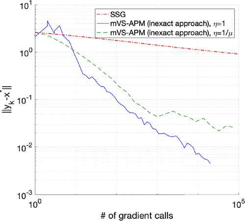
We revisit this comparison using a stochastic utility problem.

$$\underset{\Vert x\Vert \le 1}{\min }\mathbb{E}\left[\varphi \left({\displaystyle \sum _{i=1}^n\left(\frac{i}{n}+{\omega }_i\right)}{x}_i\right)\right]+\frac{\mu }{2}\Vert x{\Vert }^2,$$

where $\varphi (t)\triangleq {\max }_{1\le j\le m}(v_i+s_{i}t)$, ω_i are i.i.d. normal random variables with mean zero and variance one and $v_i,s_i\in (0,1)$. Table 5 shows similar behavior as in Example 1. In Table 6, we compare (mVS-APM) with (SSG) for different choices of standard deviation and dimension (n). In Table 6 (L), we set $\mu =0.1$, whereas n = 20, and in Table 6 (R), we set $\mu =0.1$ and standard deviation is one. Similar to Example 1, (mVS-APM) outperforms (SSG) in all cases.

Table 5. Example 2: Comparing (mVS-APM) vs. (SSG)

Table 6. Example 2: Comparing mVS-APM vs. SSG: Different Std (L), Different n (R)

4.2. sVS-APM: Convex and Smoothable f

Example 3.

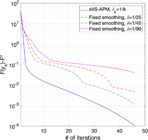
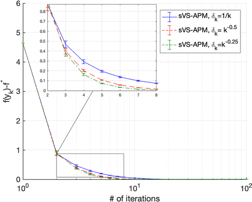
In this setting, we compare the performance of sVS-APM for merely convex problems on Example 2 with μ = 0. The δ-smoothed approximation of $\varphi (t)$ provided by Beck and Teboulle (2012) is given by ${\varphi }_{\delta }(t)=\delta \log \left({\sum }_{i=1}^m{e}^{(v_i+s_{i}t)/\delta }\right)$. In Table 7, we generate 20 replications for sVS-APM with fixed and diminishing smoothing sequences with ${\eta }_k={\delta }_k/2,\hspace{0.17em}{N}_k=\lfloor k^{3.001}\rfloor$, and sampling budget is 1e6. In Figure 3, we compare trajectories for sVS-APM with those for constant smoothing for n = 200.

Table 7. Example 3: Comparing (sVS-APM) with Fixed Smoothing

4.3. Key Observations

The empirical behavior of sVS-APM appears to be better on this test problem. One rationale for this may be drawn from noting that sVS-APM allows for larger step lengths early (because ${\eta }_k\le {\delta }_k$), whereas in the fixed smoothing technique, ${\eta }_k\le {\delta }_k$ (δ_k may be quite small). This can be seen in the trajectories in which early progress by the iterative smoothing scheme can be observed. A larger δ_k allows for larger step lengths but leads to a coarser approximation of the original problem, whereas smaller δ_k leads to poorer progress but better approximations (see Table 7 and Figure 3).

4.4. Almost Sure Convergence

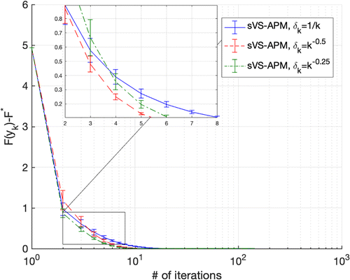
Next, we implement sVS-APM on the stochastic utility problem with n = 20 and m = 10 for different choices of the smoothing sequences. Specifically, we allow δ_k to be ${\delta }_k\in \{1/k,1/\sqrt{k},1/k^{0.25}\}$ (${\delta }_k=1/k$ is required for convergence in mean and ${\delta }_k=1/k^b$ with $b\in (0,1/2]$ for a.s. convergence). We employ $N_k=\lfloor k^{3.001}\rfloor$. For each experiment, the mean of 20 replications and their 95% confidence intervals are plotted in Figures 4 and 5. It can be seen that, when ${\delta }_k\to 0$ at a slower rate as mandated by the requirement of the a.s. convergence result, the confidence bands are tighter, becoming more apparent in Figure 4 in which the variance is five. Furthermore, our numerical studies reveal that, even for less aggressive choices of N_k such as when $N_k=k^a$ and a > 1, the trajectories show the desired behavior in accordance with Proposition 2.

5. Concluding Remarks

Drawing motivation from the often poor behavior of (SSG) schemes on general (rather than structured) nonsmooth stochastic convex optimization problems, we develop two sets of accelerated proximal variance-reduced schemes, both of which rely on a variable sample-size accelerated proximal method (VS-APM) for smooth convex problems. In nonsmooth strongly convex regimes, we present three sets of schemes, each of which produces linearly convergent sequences and is characterized by an overall complexity in subgradients (or proximal evaluations in the third case) that is optimal (or near optimal). First, in compact domains, we propose (mVS-APM), an avenue that requires applying VS-APM on the Moreau envelope of F, where increasingly exact gradients are computed via an inner (SSG) scheme. Second, in unbounded domains, we apply an unaccelerated variable sample-size proximal method (VS-PM), which also relies on (SSG) for approximating gradients to increasing accuracy. When $\tilde{f}(·,\omega )$ is smoothable and convex, our smoothed VS-APM scheme (or sVS-APM) admits optimal rate and oracle complexity. Our findings, when specialized to the smooth and convex f, provide an optimal accelerated rate of $\mathcal{O}(1/K^2)$ with optimal oracle complexity matching findings by Ghadimi and Lan (2016) and Jofré and Thompson (2017). When f is deterministic, our rate matches that obtained by Nesterov (2005b) but does so while providing asymptotically convergent schemes. Preliminary numerics suggest that the schemes compare well with existing techniques in terms of both complexity as well as sensitivity to problem parameters.

References

- (2017) First-Order Methods in Optimization (SIAM, Philadelphia).Google Scholar
- (2009) A fast iterative shrinkage-thresholding algorithm for linear inverse problems. SIAM J. Imaging Sci. 2(1):183–202.Google Scholar
- (2012) Smoothing and first order methods: A unified framework. SIAM J. Optim. 22(2):557–580.Google Scholar
- (2013) A double smoothing technique for solving unconstrained nondifferentiable convex optimization problems. Comput. Optim. Appl. 54(2):239–262.Google Scholar
- (2015) A variable smoothing algorithm for solving convex optimization problems. TOP 23(1):124–150.Google Scholar
- (2015) Convex Optimization: Algorithms and Complexity, Foundations and Trends in Machine Learning (Now Publishers, Inc., Hanover, MA), 8(3–4):231–357.Google Scholar
- (2011) A first-order primal-dual algorithm for convex problems with applications to imaging. J. Math. Imaging Vision 40(1):120–145.Google Scholar
- (2013) Bounds on the Lambert function and their application to the outage analysis of user cooperation. IEEE Comm. Lett. 17(8):1505–1508.Google Scholar
- (2015) Stochastic block mirror descent methods for nonsmooth and stochastic optimization. SIAM J. Optim. 25(2):856–881.Google Scholar
- (2012) Double smoothing technique for large-scale linearly constrained convex optimization. SIAM J. Optim. 22(2):702–727.Google Scholar
- (2014) First-order methods of smooth convex optimization with inexact oracle. Math. Programming 146(1–2):37–75.Google Scholar
- (2016) Stochastic intermediate gradient method for convex problems with stochastic inexact oracle. J. Optim. Theory Appl. 171(1):121–145.Google Scholar
- (2003) Finite-Dimensional Variational Inequalities and Complementarity Problems, Springer Series in Operations Research, vol. I (Springer-Verlag, New York).Google Scholar
- (2012) Optimal stochastic approximation algorithms for strongly convex stochastic composite optimization I: A generic algorithmic framework. SIAM J. Optim. 22(4):1469–1492.Google Scholar
- (2013) Optimal stochastic approximation algorithms for strongly convex stochastic composite optimization II: Shrinking procedures and optimal algorithms. SIAM J. Optim. 23(4):2061–2089.Google Scholar
- (2016) Accelerated gradient methods for nonconvex nonlinear and stochastic programming. Math. Programming 156(1–2):59–99.Google Scholar
- (1984) Generalized Hessian matrix and second-order optimality conditions for problems with data. Appl. Math. Optim. 11(1):43–56.Google Scholar
- (2016) eg-VSSA: An extragradient variable sample-size stochastic approximation scheme: Error analysis and complexity trade-offs. Winter Simulation Conf., 690–701.Google Scholar
- (2017) On variance reduction for stochastic smooth convex optimization with multiplicative noise. Preprint, submitted May 8, https://arxiv.org/abs/1705.02969.Google Scholar
- (2003) Stochastic Approximation and Recursive Algorithms and Applications, Applications of Mathematics, vol. 35, 2nd ed. (Springer Science & Business Media, New York).Google Scholar
- (2012) An optimal method for stochastic composite optimization. Math. Programming (Springer), 133(1):365–397.Google Scholar
- (1965) Proximité et dualité dans un espace hilbertien. Bull. Soc. Math. France 93(2):273–299.Google Scholar
- (2009) Robust stochastic approximation approach to stochastic programming. SIAM J. Optim. 19(4):1574–1609.Google Scholar
- (1983) A method for unconstrained convex minimization problem with the rate of convergence . Doklady AN USSR 269:543–547.Google Scholar
- (2005a) Excessive gap technique in nonsmooth convex minimization. SIAM J. Optim. 16(1):235–249.Google Scholar
- (2005b) Smooth minimization of non-smooth functions. Math. Programming 103(1):127–152.Google Scholar
- (2014) Introductory Lectures on Convex Optimization: A Basic Course, 1st ed. (Springer Publishing Company, Inc. Norwell, MA).Google Scholar
- (2018) Recent trends in stochastic gradient descent for machine learning and big data. Proc. 2018 Winter Simulation Conf. (IEEE Press), 366–380.Google Scholar
- (2012) Prisma: Proximal iterative smoothing algorithm. Preprint, submitted June 11, https://arxiv.org/abs/1206.2372.Google Scholar
- (2012) Stochastic smoothing for nonsmooth minimizations: Accelerating SGD by exploiting structure. Preprint, submitted May 21, https://arxiv.org/abs/1205.4481.Google Scholar
- (2016) Strongly convex functions, Moreau envelopes, and the generic nature of convex functions with strong minimizers. SIAM J. Optim. 26(2):1341–1364.Google Scholar
- (1987) Introduction to Optimization (Optimization Software, Inc., New York).Google Scholar
- (1992) Acceleration of stochastic approximation by averaging. SIAM J. Control Optim. 30(4):838–855.Google Scholar
- (1951) A stochastic approximation method. Ann. Math. Statist. 22(3):400–407.Google Scholar
- (2011) Convergence rates of inexact proximal-gradient methods for convex optimization. Adv. Neural Inform. Processes Systems 24:1458–1466.Google Scholar
- (2013) Stochastic gradient descent for non-smooth optimization: Convergence results and optimal averaging schemes. Internat. Conf. Machine Learn., 71–79.Google Scholar
- (2015) Budget-constrained stochastic approximation. Proc. 2015 Winter Simulation Conf., 368–379.Google Scholar
- (2009) Lectures on Stochastic Programming (SIAM, Philadelphia).Google Scholar
- (2017) Adaptive smoothing algorithms for nonsmooth composite convex minimization. Comput. Optim. Appl. 66(3):425–451.Google Scholar
- (2018) A smooth primal-dual optimization framework for nonsmooth composite convex minimization. SIAM J. Optim. 28(1):96–134.Google Scholar
- (2017) Smoothing technique for nonsmooth composite minimization with linear operator. Preprint, submitted June 19, https://arxiv.org/abs/1706.05837.Google Scholar
- (2010) Having fun with Lambert W(x) function. Preprint, submitted March 8, https://arxiv.org/abs/1003.1628.Google Scholar
- (2012) On stochastic gradient and subgradient methods with adaptive steplength sequences. Automatica J. IFAC 48(1):56–67.Google Scholar
- (2014) Accelerated stochastic gradient method for composite regularization. Artificial Intelligence Statist., 1086–1094.Google Scholar