Utility Maximizing Load Balancing Policies
Abstract
Consider a service system where incoming tasks are instantaneously dispatched to one out of many heterogeneous server pools. Associated with each server pool is a concave utility function that depends on the class of the server pool and its current occupancy. We derive an upper bound for the mean normalized aggregate utility in stationarity and introduce two load balancing policies that achieve this upper bound in a large-scale regime. Furthermore, the transient and stationary behavior of these asymptotically optimal load balancing policies is characterized on the scale of the number of server pools in the same large-scale regime.
Funding: This work was supported by the Netherlands Organization for Scientific Research (NWO) through [Gravitation Grant NETWORKS-024.002.003] and [Gravitation Grant Vici 202.068].
Supplemental Material: The online appendix is available at https://doi.org/10.1287/stsy.2022.0103.
1. Introduction
We consider a service system where incoming tasks are instantaneously assigned to one out of many heterogeneous server pools. All the tasks sharing a server pool are executed in parallel and the execution times do not depend on the class of the server pool or the number of tasks currently contending for service. Nevertheless, associated with each server pool is a not necessarily increasing concave utility function that does depend on the class of the server pool and the number of tasks currently sharing it. These features are characteristic of streaming and online gaming services, where the duration of tasks is mainly determined by the application, but still congestion can have a strong impact on the experienced performance (e.g., video resolution and fluency).
The goal is to assign tasks to maximize the overall utility of the system, defined as the aggregate utility of all the server pools normalized by the number of server pools. We derive an upper bound for its stationary mean through an optimization problem where the optimization variable is a sequence that describes the distribution of a fractional number of tasks across the server pools; the objective of the problem is the overall utility function, and the main constraint is that the total number of tasks must be equal to the offered load of the system. We construct an optimal (fractional) task assignment that solves this problem and has a particularly insightful structure, and we formulate the upper bound for the mean stationary overall utility in terms of this solution.
Armed with the previous insight, we propose and analyze two assignment policies that maintain the occupancy state of the system aligned with an optimal task assignment. Specifically, we examine a policy that assigns every new task to a server pool with the largest marginal utility; this policy is dubbed join the largest marginal utility (JLMU). We also introduce a multithreshold policy that follows the same greedy principle but only approximately and uses significantly less state information. The optimal threshold values depend on the typically unknown offered load of the system and are adjusted over time through an inbuilt learning scheme; thus, we name this policy self-learning threshold assignment (SLTA). Assuming exponential service times, we characterize the asymptotic transient and stationary behavior of both policies on the scale of the number of server pools, and we prove that both policies achieve the upper bound for the mean stationary overall utility as the number of server pools grows large.
A fundamental difference between JLMU and SLTA is that the former is naturally agnostic to the offered load, whereas for the latter, the optimal thresholds depend on the offered load. However, we show that the online learning scheme of SLTA is capable of finding the optimal threshold values without any prior knowledge of the offered load, which makes it possible to deploy SLTA if the offered load is not known in advance.
1.1. Main Contributions
The main contribution of this paper is an upper bound for the mean stationary overall utility that is asymptotically tight for exponentially distributed service times and thereby serves as a crucial performance benchmark. The asymptotic tightness of the upper bound is proved by studying the stationary behavior of JLMU and SLTA in the regime where the number of server pools grows large and by establishing that both assignment policies achieve the upper bound in the latter regime.
The analysis of JLMU is based on a fluid limit given by an infinite system of differential equations with a discontinuous right-hand side. We prove that the associated initial value problem always has a unique solution by making a connection with a system of integral equations, expressed in terms of Skorokhod one-dimensional reflection mappings and using a uniqueness result for certain Kolmogorov backward equations. Moreover, we show that the fluid limit holds with respect to an norm and that the system of differential equations is globally asymptotically stable with respect to this norm. These results are used to prove that the stationary distribution of the process that describes the occupancy state of the system converges in to an optimal task assignment for the offered load of the system. The asymptotic optimality of JLMU is then established by proving that the stationary overall utilities form a convergent and uniformly integrable sequence of random variables; the proof of the latter properties exploits a representation of the overall utility as a linear functional on and our convergence results with respect to the norm.
Although SLTA is simple to implement, its analysis is inherently challenging due to the complex interdependence between two components of the policy. Namely, the dispatching rule, which depends on the multiple thresholds, and the online learning scheme, which adjusts the thresholds over time. Furthermore, an additional technical difficulty is that the learning scheme is triggered by excursions of the occupancy state of the system that asymptotically vanish on the scale of the number of server pools.
To analyze the large-scale transient behavior of SLTA, we use a methodology of Goldsztajn et al. (2021a) that allows overcoming of the aforementioned challenges by means of a nontraditional fluid limit analysis. In this paper, we extend the latter methodology to also prove weak convergence of the stationary distribution of the occupancy process and thresholds. Here our contributions are proofs of ergodicity and tightness of stationary distributions through a careful drift analysis, as well as a suitably adapted interchange of limits argument designed to leverage the large-scale transient result obtained with the methodology of Goldsztajn et al. (2021a). Equipped with the convergence results for the stationary distributions, we prove the asymptotic optimality of SLTA in a similar way as for JLMU by showing that all our limit theorems hold with respect to the norm and exploiting the linear representation of the overall utility function.
1.2. Related Work
Load balancing and task assignment in parallel-server systems has received immense attention in the past decades; some relevant papers are Winston (1977), Vvedenskaya et al. (1996), Mitzenmacher (2001), Lu et al. (2011), Stolyar (2015), and Eschenfeldt and Gamarnik (2018). Traditionally the focus used to be on performance, but more recently the implementation overhead has emerged as an equally important issue. In large-scale deployments, this overhead has two main sources: the communication burden of messaging between the dispatcher and the servers and the operational cost of storing and managing state information at the dispatcher (Gamarnik et al. 2018, 2020). We refer to Van der Boor et al. (2022) for an extensive survey on scalable load balancing.
Whereas the load balancing literature has been predominantly concerned with systems of parallel single-server queues, the present paper considers an infinite-server setting where the service times of tasks do not depend on the number of competing tasks. As noted earlier, this feature is characteristic of streaming applications, where the level of congestion does not significantly affect the duration of tasks. The level of congestion has, however, a strong impact on the amount of resources received by individual streaming sessions, and thus on the experienced quality-of-service, which can be modeled through utility functions. Infinite-server dynamics have been commonly adopted as a natural paradigm for modeling streaming sessions on flow-level (Benameur et al. 2002, Key et al. 2004), and the problem of managing large data centers serving streaming sessions has been recently addressed in Mukherjee et al. (2020). Systems with infinite-server dynamics have also been analyzed in Mukhopadhyay et al. (2015a, b), Karthik et al. (2017), and Xie et al. (2015), which concern loss models that are different in nature from the setting considered in the present paper.
When the server pools are homogeneous, the overall utility is a Schur-concave function of the vector describing the number of tasks at each server pool. In this case, maximizing the aggregate utility of the system boils down to equalizing the number of tasks across the various server pools. Join the shortest queue (JSQ) maximizes the mean stationary overall utility of the system for exponential service times and, in fact, has stronger stochastic optimality properties (Menich and Serfozo 1991, Sparaggis et al. 1993). In the homogeneous setting, JLMU reduces to JSQ and is thus optimal for exponential service times. In addition, SLTA reduces to the policy considered in Goldsztajn et al. (2021a, b), which asymptotically matches the performance of JSQ on the fluid and diffusion scales for exponentially distributed service times. Although the policy considered in Zhou et al. (2017, 2018) and Horváth et al. (2019) is similar to SLTA in name, this policy does not equalize the queue lengths.
The problem of maximizing the overall utility of the system is more challenging if the server pools are heterogeneous as in this paper. Heterogeneity is the norm in data centers, where servers from different generations coexist because old machines are only gradually replaced by more powerful versions; as shown in Figure 1, this feature has been recently addressed in the load balancing literature for single-server models (Gardner and Stephens 2019, Jaleel et al. 2020, Gardner et al. 2021) but not in the infinite-server context. When the server pools are heterogeneous, it is no longer optimal to maintain an evenly balanced distribution of the load; in fact, it is not even obvious at all how tasks should be distributed to maximize the overall utility function, and the optimal distribution of tasks across the server pools depends on this function. Another striking difference with the homogeneous setting is that JLMU is generally not optimal in the prelimit for exponentially distributed service times; we establish that, in general, the optimality is only achieved asymptotically in the heterogeneous case.
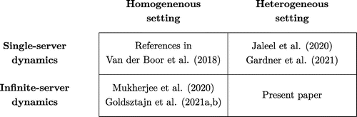
Notes. Most of the load balancing literature concerns systems of parallel and homogeneous single-server queues; this vast literature is surveyed in Van der Boor et al. (2022). Some recent papers study single-server dynamics in heterogeneous settings or infinite-server dynamics in homogeneous settings, whereas the present paper considers a heterogeneous system with infinite-server dynamics.
From a theoretical perspective, one of the most interesting features of SLTA is its capacity to learn the offered load of the system. The problem of adaptation to unknown demands was previously addressed in Mukherjee et al. (2017) and Goldsztajn et al. (2018, 2022) in the context of single-server models by assuming that the number of servers can be right-sized on the fly to match the load of the system. However, in the latter papers the dispatching rule remains the same at all times because the right-sizing mechanism alone is sufficient to maintain small queues, by adjusting the number of servers. Different from these right-sizing mechanisms, the learning scheme of SLTA modifies the parameters of the dispatching rule over time to maximize the overall utility of the system.
1.3. Outline of the Paper
In Section 2, we introduce some of the notation used throughout the paper and we prove the upper bound for the mean stationary overall utility. In Section 3, we specify the JLMU and SLTA policies, and we state their asymptotic optimality with respect to the mean stationary overall utility. In Section 4, we present several results that pertain to the asymptotic transient behavior of these two policies and that are used to establish their asymptotic optimality. To characterize the asymptotic behavior of JLMU and SLTA, we construct systems of different sizes on a common probability space in Section 5, where we also prove relative compactness results. Limit theorems for the transient regimes of JLMU and SLTA are proved in Sections 6 and 7, respectively, and the asymptotic optimality of these policies is established in Section 8. Some proofs are deferred to Online Appendices A, B and C.
2. Performance Upper Bound
In this section, we define some of the notation used throughout the paper and we prove the upper bound for the mean stationary overall utility. In Section 2.1, we introduce two descriptors for specifying the state of the system, and we define the overall utility function. In Section 2.2, we present the optimization problem used to derive the upper bound for the mean stationary overall utility. In Section 2.3, we construct a solution of this problem explicitly, and in Section 2.4, we use the constructed solution to formulate the upper bound for the mean stationary overall utility, which we prove in Section 2.5.
2.1. Basic Notation
Consider a system with m classes of server pools. All the tasks sharing a server pool are executed in parallel and the execution times do not depend on the class of the server pool or the number of tasks currently contending for service. Nevertheless, associated with each server pool is a concave utility function which does depend on the class of the server pool and the number of tasks sharing it. For example, these functions can be used to model the overall quality-of-service provided to streaming tasks sharing an underlying resource with a fixed capacity. The objective is to assign the incoming tasks to the various server pools to maximize the aggregate utility of all the server pools in stationarity.
The number of server pools is denoted by n, and the number and fraction of server pools of class i are denoted by and , respectively. We assume that tasks arrive as a Poisson process of intensity with independent and identically distributed service times of mean , and we define as the number of tasks in server pool k of class i; bold symbols are used in the paper to indicate time dependence. Server pools of the same class that have the same number of tasks are exchangeable; thus, we usually consider a different state descriptor. Specifically, we let
The concave utility function associated with server pools of class i is denoted by ui, and the overall utility of the system is defined as the aggregate utility of all the server pools normalized by the number of server pools. More precisely, we let
Note that is the fraction of server pools of class i with j tasks. Thus, the overall utility may equivalently be expressed as
Although the overall utility function is generally not linear as a function of , it is always linear as a function of , as shown by the previous expression.
The total number of tasks in the system, normalized by the number of server pools, can be expressed in terms of the occupancy state as follows:
The quantity represents the number of tasks in server pools of class i with exactly j tasks, normalized by the total number of server pools. Hence, indeed corresponds to the normalized total number of tasks.
Throughout the paper, we write and to denote the probability and expectation with respect to a given probability measure. If denotes the normalized offered load, then the stationary distribution of the total number of tasks is Poisson with mean due to the infinite-server dynamics of the system. Thus, in stationarity, for any task assignment policy.
2.2. Optimization Problem
Based on the previous statements, we now formulate an optimization problem that yields an upper bound for the mean stationary overall utility:
To see that the optimum of (2) yields an upper bound for the mean stationary overall utility, consider any policy such that has a stationary distribution. We assume that the policy is such that the evolution of the system over time can be described by a Markov process, with a possibly uncountable state space, that has a stationary distribution. Let qn be a random variable with the stationary distribution of and define as the sequence whose (i, j) element is . Observe that
Indeed, the utility functions are concave, so for each i there exists such that and have the same sign if . Therefore, (3) follows from Tonelli’s theorem. In addition, satisfies the constraints of (2) because the total number of tasks in stationarity has mean . Thus, is upper bounded by the optimum of (2).
2.3. Structure of an Optimal Solution
For brevity, we refer to an optimizer of (2) as an optimal task assignment; the term optimal fractional task assignment would be more appropriate since the offered load may not be integral. In this section we define a ranking of the server pools that can be used to construct an optimal task assignment. For this purpose, consider the sets
A server pool has coordinates if its class is i and it has precisely tasks; for example, in Figure 2, server pool A of class 1 has coordinates (1, 4), and both server pools of class 3 have coordinates (3, 1). Because server pools with the same coordinates are statistically identical, we may focus on ranking coordinates rather than server pools.
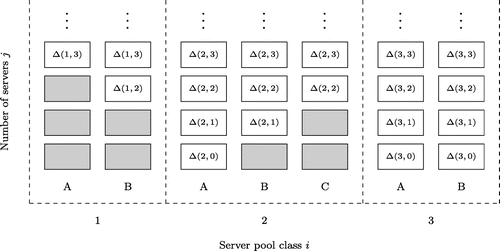
Notes. White rectangular slots and gray rectangles represent idle and busy servers, respectively. Each of the columns labeled with letters represents a server pool and the dashed lines enclose server pools of the same class. If the tasks sent to a given server pool are always placed in the first idle server from bottom to top, then the marginal utilities written on top of the idle servers indicate the increase in the aggregate utility of the system when the server receives a task.
Formally, we define a total order on that gives precedence to coordinates associated with larger marginal utilities. The marginal utility of a server pool of class i with j tasks is denoted by and represents the change in the utility function of such a server pool if it receives an additional task. The marginal utility of the coordinates (i, j) is just , the marginal utility of server pools of class i with tasks.
Consider the dictionary order on , defined by
We obtain a total order on by writing if and only if one of the following conditions holds:
In particular, the marginal utility of server pools with coordinates (i1, j1) is smaller than or equal to that of server pools with coordinates . The dictionary order is used to break the tie when both coordinates are associated with the same marginal utility, but a different tie breaking rule could be used instead.
Consider the task assignment defined by
In Section 2.5, we prove that constitutes an optimal task assignment if is defined as the unique element of that satisfies
For the uniqueness of , the number of terms in the summations on both sides of (4) increases as the ranking of becomes worse and that the summation on the right has exactly one more term than the summation on the left.
2.3.1. Numerical Examples.
Figure 3 depicts the optimal task assignments obtained through (4) for two sets of utility functions and different values of ρ. If n is such that and are integers for all i, then the plots can be interpreted as sets of n adjacent columns, where each column represents a server pool and the colored portion of a column indicates the number of tasks sharing the server pool, as in the diagram of Figure 2. The thick vertical lines separate the server pool classes and the quantities can be read off by rotating the plots.
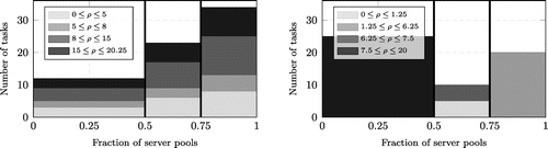
Notes. (Left) with . (Right) if x < 20 and if . In both cases m = 3 and .
The left plot corresponds to utility functions of the form , with g a concave and increasing function. These utility functions can be used to model the aggregate quality-of-service provided to streaming tasks sharing a single server pool. The quantity r(i) represents the total amount of resources in a server pool of class i and models the quality-of-service provided to a single task when the server pool is shared by x tasks and each task gets a fraction of the total resources. For a given ρ, the left plot of Figure 3 depicts server pools with roughly tasks, with a normalizing constant that does not depend on g; for some values of ρ, all server pools have exactly tasks, but in other cases some of these numbers are rounded. This behavior is explained by noting that the derivative of can be expressed as a function of , thus the occupancy levels equalize the marginal utilities.
In the left plot of Figure 3, the occupancy levels of the various server pools maintain approximately fixed ratios as ρ increases. The right plot shows a completely different behavior: as ρ increases from 0 to 1.25, only the occupancy of server pools of class 2 grows, but from 1.25 to 6.25, only the occupancy of server pools of class 3 grows, and eventually exceeds the occupancy of server pools of class 2. Furthermore, as ρ increases beyond 7.5, only the occupancy of server pools of class 1 increases.
2.4. Performance Upper Bound
We now state the upper bound for the mean stationary overall utility. The proof uses the remarks of Sections 2.2 and 2.3 and is given in Section 2.5.
Consider any task assignment policy such that the occupancy process has a stationary distribution and let qn be a random variable distributed as this stationary distribution. Then
In Section 3.4, we establish that the upper bound is asymptotically achievable when service times are exponentially distributed. In particular, we will see that JLMU achieves the upper bound of Theorem 1 as the number of server pools grows large; recall that JLMU is generally not optimal in the prelimit, not even for exponential service times. Moreover, we will establish that SLTA also achieves the upper bound asymptotically while relying on considerably less state information.
2.5. Proof of the Upper Bound
Recall from Section 2.2 that the optimum of (2) is an upper bound for the mean stationary overall utility. Therefore, we only need to prove that the task assignment defined in (4) is an optimizer of (2). For this purpose, we introduce the following definition. We say that a sequence is eventually zero if there exists k > 0 such that for all i and j > k. The following lemma implies that is an optimizer of (2) if we impose the additional constraint that the solution must be eventually zero.
If q satisfies the constraints of (2) and is eventually zero, then .
Because q is eventually zero, it is possible to write
In the last expression, the terms of the summation are ordered with respect to and in particular in nonincreasing order of the marginal utilities . The task assignment is obtained by choosing the coefficients q(i, j) so that the first coefficients are maximal while all the coefficients add up to ρ. Thus, maximizes the right-hand side of (6). □
We now provide a solution of (2), without imposing any additional constraints.
By Lemma 1, it suffices to prove that for each q that is not eventually zero and satisfies the constraints of (2). Next, we fix one such sequence q and we construct an eventually zero sequence z such that and z satisfies the constraints of (2). Then by Lemma 1, as desired.
Choose such that for all i. For each i, we define z(i, j) iteratively, by
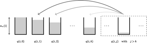
Informally, each coefficient q(i, j) can be regarded as a container with capacity , as shown in Figure 4. For each i, the sequence is transformed into in two steps: first we remove all the mass from the coefficients q(i, j) with j > k, and then we place this mass on the coefficients q(i, j) with . In the latter step, we start with the first coefficient, placing as much mass as possible without exceeding the capacity . The remainder of mass is placed in the following coefficients in the same fashion, and in increasing order of j. Observe that all the mass will have been placed right after the coefficient q(i, k) is done because q satisfies the constraints of (2) and . Furthermore, the following property holds:
The overall utility of the task assignment q satisfies
For the last step, recall that z is eventually zero, so u(z) can be computed as in (6). Note that and if . Therefore,
The middle equality and last inequality follow from (7) and Lemma 1, respectively. □
The proof of Theorem 1 follows easily from Proposition 1.
As indicated at the end of Section 2.2, the optimum of (2) upper bounds the mean stationary overall utility . Thus, it follows from Proposition 1 that upper bounds the mean stationary overall utility. □
3. Load Balancing Policies
In this section we describe the load balancing policies considered in the paper, and we state their asymptotic optimality with respect to the mean stationary overall utility when service times are exponential. In Sections 3.1 and 3.2, we specify JLMU and SLTA, respectively. In Section 3.3, we define stochastic models, based on continuous-time Markov chains, for the analysis of both policies. In Section 3.4, we state the asymptotic optimality result.
Before proceeding, it is illustrative to draw an analogy between the setting considered in this paper and the load balancing literature for systems of parallel single-server queues, where the primary objective is to minimize queueing delay. The natural policy for the setting considered in this paper is JLMU, while the natural policy for minimizing queueing delay in systems of parallel single-server queues is JSQ. The deployment of these policies involves a considerable communication overhead, or storing and managing a significant amount of state information. In the setting considered in this paper, SLTA provides a asymptotically optimal performance for exponential service times and uses substantially less state information than JLMU. From this perspective, SLTA is the counterpart of JIQ in the load balancing literature for systems of parallel single-server queues (Lu et al. 2011, Stolyar 2015).
3.1. Join the Largest Marginal Utility (JLMU)
JLMU assigns every new task to a server pool that currently has the best ranked coordinates, thus also the largest marginal utility. Formally, define
The coordinates obtained through (8) correspond to server pools with the largest marginal utility by definition of . In addition, observe that the dictionary order is used to break ties between coordinates associated with the same marginal utility. If two server pools have the same coordinates, then it does not matter which of them is assigned the new task since they are statistically identical. For definiteness, we postulate that the tie is broken uniformly at random.
If all the server pools have the same utility function, then JLMU reduces to JSQ, and the overall utility is a Schur-concave function of . If in addition the service times are exponential, then the stochastic optimality properties proved in Sparaggis et al. (1993) and Menich and Serfozo (1991) for JSQ imply that JLMU maximizes the mean stationary overall utility in this homogeneous setting. It might be natural to expect that the optimality with respect to the mean stationary overall utility extends to the heterogeneous setting. We refute this, however, in Section 8.3, where we construct a heterogeneous system for which JLMU is strictly suboptimal. The constructed example also hints at the underlying reasons for the suboptimality in the heterogeneous case. Essentially, instead of always assigning incoming tasks greedily, such that the increase in the overall utility is maximal, it is sometimes advantageous to dispatch the new tasks conservatively, to hedge against pronounced drops of the overall utility that may be caused by a quick succession of departures. The right balance between greedy and conservative actions depends intricately on the utility functions, but we prove that JLMU is always asymptotically optimal for exponential service times, regardless of the specific set of utility functions; this result is stated formally in Section 3.4.
3.2. Self-Learning Threshold Assignment (SLTA)
JLMU relies on complete information about the number of tasks per server pool, which could be impractical in large-scale deployments. In contrast, SLTA only requires to store at most two bits per server pool, which is considerably less state information. To specify this policy, we need to describe its two components. Namely, the dispatching rule, for assigning the incoming tasks to the server pools, and the learning scheme, for dynamically adjusting a set of thresholds that the dispatching rule uses.
Consider the unique enumeration of such that for all k. Given , we define a set of thresholds by
Recall the optimal task assignment defined at the end of Section 2.3. The learning scheme keeps an estimate of the coordinates , which depend on the typically unknown offered load of the system. The index determines this estimate and is used to compute thresholds from the previous expression, which are in turn used to assign tokens to the server pools. Specifically, a server pool of class i with exactly tasks has
A green token if ,
A yellow token if and .
The first condition is equivalent to and , and the second condition is equivalent to and . Also, a server pool can have both a green and a yellow token at the same time. As indicated in Figure 5, a larger increase in the overall utility is obtained by dispatching tasks to server pools with green tokens first, then to server pools with yellow tokens and only afterward to server pools without tokens.
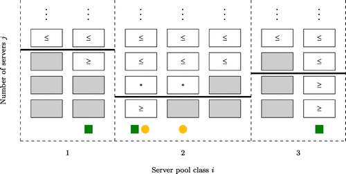
Notes. The thresholds are indicated by thick horizontal lines that cross the server pools, and the tokens are represented using squares and circles underneath the server pools; a square corresponds to a green token and a circle corresponds to a yellow token. Assuming that the rectangular slots within a server pool are always filled from bottom to top, the slots marked with an provide a marginal utility of . The symbols and indicate how the marginal utility of the other slots compares to the latter value.
The tokens are used by the dispatching rule. Specifically, when a task arrives, it is assigned to a server pool according to the following criteria.
In the presence of green tokens of class , the dispatcher picks one of these green tokens uniformly at random, and if only green tokens of class remain, then one of these is picked. Then the task is sent to the corresponding server pool.
In the presence of only yellow tokens, the dispatcher picks a yellow token uniformly at random and sends the task to the corresponding server pool.
Otherwise, the task is sent to a server pool chosen uniformly at random.
If are the coordinates defined in (5), then this dispatching rule drives the occupancy state of the system toward the optimal task assignment specified in (4).
The learning scheme aims at finding the coordinates , which depend on the typically unknown offered load. The learning scheme is parameterized by and adjusts the value of at certain arrival epochs, in steps of one unit. Specifically, when a task arrives, the learning scheme acts only under the following circumstances.
If the system has at least green tokens and at least one belongs to a server pool of class , then is decremented by one after the task is dispatched.
If the number of yellow tokens is smaller than or equal to one and there are no other tokens, then is incremented by one after the task is dispatched.
Observe that exactly one of the thresholds changes when the value of is modified and that this threshold changes by one unit. Also, note that
3.2.1. Comparison with the Homogeneous Case.
When all the server pools are of the same class, SLTA reduces to the load balancing policy studied in Goldsztajn et al. (2021a). In this case, there is a single threshold whose optimal value is simply . When the threshold has this value, the number of green tokens and the total number of tokens are typically small and positive, respectively. On the other hand, when the threshold is below optimal, the total number of tokens tends to be zero, and when the threshold is larger than optimal, the number of green tokens tends to be relatively large. These properties are used to adjust the threshold in an online manner when the offered load is unknown. In few words, the threshold is increased in the absence of tokens, and it is decreased if the number of green tokens is large enough.
In the general case, there are as many thresholds as the number of server pool classes, and the optimal threshold values depend intricately on the utility functions and the offered load. However, the ranking introduced in Section 2.3 makes it possible to express all the thresholds as a function of the coordinates . Hence, the optimal thresholds can still be found through a one-directional search, but now in the totally ordered space . Moreover, because this space is countable, the search can be carried out by adjusting the integral parameter until reaches the optimal value .
The learning scheme of SLTA operates so that all the thresholds are at their optimal values if and only if is at its optimal value, and when this happens, the number of green tokens and the total number of tokens are typically small and positive, respectively. When is below optimal, all the thresholds are smaller than or equal to their optimal values, and at least one of the thresholds is strictly smaller than optimal; in this case, the total number of tokens tends to be zero. Similarly, when is above optimal, all the thresholds are larger than or equal to their optimal values and at least one of the thresholds is above optimal; as a result, the number of green tokens tends to be relatively large. As in the homogeneous case, these observations are used to adjust over time. Loosely speaking, in the absence of tokens, is increased by one unit, which implies that one of the thresholds is increased by one unit, and when the number of green tokens is large enough, is decreased by one unit, and thus one of the thresholds is decreased by one unit.
The dispatching rule and the online learning scheme of SLTA make distinctions between green tokens of class and green tokens of any other class. The rationale is that the marginal utility of server pools of class i with tasks is the lowest when ; thus, it makes sense to give green tokens of this class the lowest priority for receiving new tasks. Although this may slightly improve performance, it is not crucial. Nevertheless, the differential treatment of class simplifies the mathematical analysis of SLTA. In particular, the distinction made in the description of the learning scheme ensures that if the system had yellow tokens, then it will continue to have yellow tokens after is decreased, which is used in Remark 1. In addition, the differential treatment by the dispatching rule simplifies the proof of Proposition 6.
3.3. Stochastic Models
If service times are exponentially distributed, then and are continuous-time Markov chains when the load balancing policies are JLMU and SLTA, respectively. In either case, the process that describes the normalized total number of tasks is defined by (1). Due to the infinite-server dynamics of the system, has the law of an queue with arrival rate and service rate μ.
Let be the space of absolutely summable sequences in , equipped with the norm
Throughout we assume that is finite, so takes values in . As a result, if we let , then takes values in the set
If the load balancing policy is JLMU, then the state space of is defined as the subset Sn of Qn that is reachable from an empty occupancy state. If the load balancing policy is SLTA, then the state space of is the subset Sn of that is reachable from an empty occupancy state with .
The notation used for the processes and , for the state space Sn, and for some other objects that will be defined later, is exactly the same for JLMU and SLTA, but we always indicate which policy is being considered.
3.4. Asymptotic Optimality
Throughout the rest of the paper, we assume that there exist constants and a random variable q0 such that the following limits hold:
In analogy with (5) and (4), we consider the unique such that
In Section 8.1, we establish that and have a unique stationary distribution for all n when the assignment policies are JLMU and SLTA, respectively. The following theorem is proved in Section 8.2 and implies that both policies are asymptotically optimal if the marginal utilities are bounded, and the service times are exponentially distributed; we also require that (9) holds, and we impose some mild technical assumptions, to be stated in Section 4.2.1. The condition on the marginal utilities always holds when the utility functions are nondecreasing due to the concavity of these functions.
Suppose that service times are exponentially distributed. Also, if the load balancing policy is SLTA, assume that the assumptions of Section 4.2.1 hold and that
The following statements hold in the asymptotic regime described by (9).
(a) Suppose that JLMU is used and let qn have the stationary distribution of . Then the random variables qn converge weakly in to .
(b) Suppose that SLTA is used and let (qn, rn) have the stationary distribution of . The random variables (qn, rn) converge weakly in to .
(c) Furthermore, if the load balancing policy is either JLMU or SLTA and the marginal utilities are bounded, then the random variables are uniformly integrable and
The claims concerning the stationary overall utilities are proved using (a) and (b), as well as the fact that u(q) is a bounded linear functional of . To establish (a) and (b), we first use drift analysis to prove that the random variables in (a) and (b) are tight in and , respectively. Then (a) is established through an interchange of limits argument based on a fluid limit and a global asymptotic stability result for the fluid dynamics; these two results are stated in Theorems 5 and 4, respectively. A different type of argument is used to prove (b). Namely, the fluid limit step is circumvented, and Theorem 6 serves as the counterpart of Theorems 4 and 5, as illustrated in Figure 6.
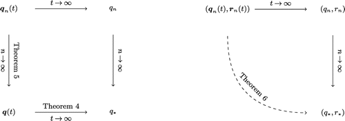
Deriving a fluid limit for a SLTA system would be inherently difficult due to the intricate interdependence between the dispatching rule and the learning scheme and because the actions of the learning scheme are triggered by excursions of the occupancy process that have vanishing size. We deal with these challenges using a methodology of Goldsztajn et al. (2021a) to derive the fluid approximation of Theorem 6, which consists of asymptotic bounds, over arbitrarily long intervals of time, for the occupancy state and the thresholds. As noted earlier, this fluid approximation serves as a counterpart of both the fluid limit and the global asymptotic stability results for JLMU.
3.4.1. Simulation Experiments.
The asymptotic optimality of JLMU and SLTA is illustrated by Table 1, which shows estimates of the mean stationary overall utility for simulation experiments with different values of n. All the estimates correspond to systems with two server pool classes of equal size and utility functions of the form for . Also, two different values of ρ are considered, so that the optimal task assignment defined in (4) takes two distinct forms. For , the optimal task assignment is such that all server pools of class 1 have 8 tasks, half of the server pools of class 2 have 11 tasks, and the other half have 12 tasks. For ρ = 10, the optimal task assignment is such that all server pools of class 1 have 8 tasks and all server pools of class 2 have 12 tasks.
|

Table 1. Results of Simulation Experiments with Different Values of n
| n | ||||||
|---|---|---|---|---|---|---|
| JLMU | SLTA | JLMU | SLTA | |||
| 50 | 9.1752 | 9.1652 | 9.1649 | 9.1594 | 9.1433 | 9.1439 |
| 100 | 9.1746 | 9.1699 | 9.1698 | 9.1627 | 9.1499 | 9.1498 |
| 150 | 9.1738 | 9.1706 | 9.1705 | 9.1633 | 9.1534 | 9.1534 |
| 200 | 9.1743 | 9.1723 | 9.1723 | 9.1634 | 9.1556 | 9.1555 |
| 250 | 9.1735 | 9.1720 | 9.1720 | 9.1639 | 9.1572 | 9.1572 |
| 300 | 9.1738 | 9.1727 | 9.1726 | 9.1613 | 9.1548 | 9.1547 |
| 350 | 9.1742 | 9.1734 | 9.1734 | 9.1619 | 9.1563 | 9.1562 |
| 400 | 9.1734 | 9.1728 | 9.1728 | 9.1632 | 9.1578 | 9.1578 |
| 450 | 9.1737 | 9.1732 | 9.1731 | 9.1630 | 9.1576 | 9.1576 |
| 500 | 9.1726 | 9.1721 | 9.1721 | 9.1632 | 9.1583 | 9.1583 |
Notes. The systems considered have two server pool classes of equal size and utility functions of the form with . Service times are exponentially distributed with μ = 1 and the time averages are computed over intervals of length 180 with equilibrium initial conditions. The same sequences of interarrival and service times were used in the simulation experiments for JLMU and SLTA. Also, in the simulations for SLTA. The upper bound of Theorem 1 for a normalized offered load of x is denoted by .
All the server pools of the same class have the same number of tasks when ρ = 10, and thus we say that the optimal task assignment is integral; that is, the optimal task assignment is integral if . In contrast, the optimal task assignment is fractional when because server pools of class 2 may have either 11 or 12 tasks. Server pools of class 1 behave similarly in the fractional and integral settings: almost all of the time all server pools of class 1 have precisely eight tasks when n is moderately large. However, the behavior of server pools of class 2 depends on the setting. In the fractional case, server pools typically have 11 or 12 tasks and the fractions of server pools with 11 and 12 tasks oscillate around a half. In the integral case, server pools typically have 12 tasks but a small number of server pools sometimes have 11 or 13 tasks instead. The aggregate utility of the system decreases by whenever a server pool of class 2 goes from 12 to 11 tasks and increases by the same quantity when the server pool goes from 11 to 12 tasks. Therefore, the contributions to the average overall utility of the oscillations observed in the fractional case roughly balance each other. In the integral case, the aggregate utility increases by , instead of , if a server pool of class 2 goes from 12 to 13 tasks. Therefore, in the integral case, the contributions to the average overall utility of class 2 server pools that drop to 11 tasks or reach 13 tasks are amplified by different marginal utilities. As a result, the mean stationary overall utility is closer to the upper bound in the fractional case, as reflected by the estimates in Table 1.
Although there is a difference between the fractional and integral settings, in both settings, the empirical mean of the overall utility is extremely close to the upper bound across all the values of n listed in Table 1. Furthermore, the deviation of the empirical mean from the upper bound approaches zero as n increases in both cases. We also observe that the empirical mean of is almost the same for JLMU and SLTA in all the experiments and particularly for the largest values of n.
A final remark on the simulation experiments is that the empirical mean of is slightly larger than in a few of the experiments within the fractional setting: both for JLMU and SLTA when n = 350 and just for JLMU when n = 450. It may be checked that the statement of Theorem 1 still holds if the stationary expectation sign is replaced by a time average and the upper bound is computed through (4) and (5) but with ρ replaced by the time average of ; the proof does not change. The value of the upper bound when ρ is replaced by the time average of is displayed in Table 1, and in all the experiments, the empirical mean of is indeed smaller than this empirical upper bound. Thus, the experiments where the empirical mean of slightly exceeds the upper bound are an indication of how close the performance of JLMU and SLTA is to optimal.
4. Approximation Theorems
In this section, we assume exponential service times and we state several results used to prove Theorem 2. In Section 4.1, we specify a fluid model of a JLMU system, based on differential equations, and we state some properties of this model. In Section 4.2, we state limit theorems that characterize the asymptotic transient behavior of JLMU and SLTA.
4.1. Fluid Model of JLMU
Consider a large-scale system where the load balancing policy is JLMU and assume that is the fraction of server pools of class i. Then the occupancy state of the system remains within the set
The evolution of the occupancy state of this large-scale system can be modeled through the system of differential equations introduced in the following definition.
We say that is a fluid trajectory if the coordinate functions are absolutely continuous for all and the following conditions hold almost everywhere with respect to the Lebesgue measure:
In the latter definition, λ is the arrival rate of tasks normalized by the number of server pools, μ is the service rate of tasks, and represents the fraction of server pools that are of class i and have at least j tasks. Thus, the system of Differential Equations (12) has a simple interpretation. The right-most term of (12a) corresponds to the departure rate of tasks from server pools of class i with exactly j tasks, and represents the arrival rate of tasks to server pools that belong to class i and have precisely tasks. The definition of Λ is motivated by the following remarks.
Server pools of class i with exactly tasks are not assigned additional tasks if . Hence, we should have in this case.
All server pools of class i have at least j tasks if . Therefore, should be equal to the last term of (12a) in this case, because is at its maximum value and thus its derivative should be zero.
The total arrival rate of tasks normalized by the number of server pools is equal to λ, and this determines the value of when .
4.1.1. Properties of Fluid Trajectories.
The two results stated here are proved in Section 6.1. The first one is a uniqueness theorem for the solutions of (12). Existence is ensured by Theorem 5 of Section 4.2.
Fix an initial condition . If there exists a fluid trajectory such that , then this fluid trajectory is unique.
To prove this theorem, we first show that all fluid trajectories satisfy an infinite system of integral equations, stated using Skorokhod one-dimensional reflection mappings. The theorem is then proved using a Lipschitz property of these mappings and a uniqueness result for certain Kolmogorov backward equations.
Besides uniqueness of solutions of (12), we also establish that there exists a unique equilibrium point and that this equilibrium point is globally asymptotically stable; that is, all fluid trajectories converge to the unique equilibrium over time.
Let be as in (11). Then is the unique equilibrium of (12). Furthermore, all fluid trajectories converge to in over time.
Recall that (11) is the counterpart of (4), which is used to formulate the upper bound for the mean stationary overall utility provided in Theorem 1. It is not difficult to check that as n grows large, which hints at the asymptotic optimality of JLMU.
4.2. Limit Theorems
In Section 5.1, we construct the processes defined in Section 3.3 on a common probability space for all n, in such a way that the sample paths of the occupancy processes lie in the space of càdlàg functions with values in , which we endow with the topology of uniform convergence over compact sets. This construction is used to prove limit theorems that characterize the asymptotic transient behavior of JLMU and SLTA. Before stating these theorems, we introduce some mild technical assumptions.
4.2.1. Technical Assumptions.
As indicated earlier, we assume that (9) holds with q0 a random variable that takes values in Q and represents the limiting initial occupancy state. The initial number of tasks in the limit, normalized by the number of server pools, is defined as
If the load balancing policy is SLTA, then we assume that the first inequality in (10) is strict and that there exists a constant such that
These assumptions are used to prove that the learning scheme reaches an equilibrium in all large enough systems with probability one. Finally, we adopt the following assumptions about the initial state of the system: There exists a random variable such that
Property (15b) is preserved by arrivals and departures; thus, it holds at all times provided that it holds at time zero. Furthermore, every new task is sent to a server pool with coordinates if the number of tokens is positive right before the arrival. Hence, (15b) implies that tasks are sent to server pools with coordinates at all times and for all n with a probability of one.
4.2.2. Statements of the Theorems.
First we state a fluid limit for JLMU, proven in Section 6.2. In view of Theorem 4, this fluid limit implies that, as n grows large, the occupancy processes of JLMU approach functions that converge over time to the unique equilibrium of (12).
Suppose that the load balancing policy is JLMU. Then there exists a set of probability one Γ with the following property. If , then converges in to the unique fluid trajectory with initial condition .
Because q0 is arbitrary, the previous theorem implies that solutions to (12) exist for all initial conditions. Therefore, Theorems 3 and 5 imply that for each initial condition there exists a unique fluid trajectory with initial condition q.
The proof of Theorem 5 uses a methodology of Bramson (1998) to prove that, with a probability of one, every subsequence of has a further subsequence that converges uniformly over compact sets with respect to a metric for the product topology of . Then we show that this convergence in fact holds with respect to and that the limits of convergent subsequences are fluid trajectories, also with a probability of one.
The counterpart of Theorems 4 and 5 for SLTA is the following result. The proof is provided in Section 7.2 and is based on a methodology of Goldsztajn et al. (2021a).
Suppose that the load balancing policy is SLTA and let and be as in (10). There exist and a set of probability one Γ with the following property. If and , then the next limits hold:
5. Strong Approximations
In this section, we construct the processes defined in Section 3.3 on a common probability space for all n. In addition, we prove that is almost surely relatively compact in both for JLMU and SLTA. The construction of the processes is carried out in Section 5.1, and the relative compactness results are provided in Section 5.2.
5.1. Coupled Construction of Sample Paths
Consider the following stochastic processes and random variables.
Driving Poisson processes: A collection of independent Poisson processes with unit rate, for counting arrivals and departures. These processes are defined on a common probability space .
Selection variables: A family of independent random variables, uniformly distributed on and defined on a common probability space .
Initial conditions: Sequences and for SLTA of random variables for describing the initial states of the systems, defined on a common probability space and satisfying the assumptions of Section 4.2.1.
Denote the completion of the product probability space of and by . The processes introduced in Section 3.3 are constructed on the latter space as deterministic functions of the stochastic primitives.
5.1.1. Construction for JLMU.
Let for each and each n. This quantity will be used to count the number of tasks arriving to the system with n server pools during the interval . Also, denote the jump times of by and define . For each function and each n, we define two counting processes, for arrivals and departures, denoted and , respectively. The coordinates of these processes are identically zero if j = 0, whereas the other coordinates are defined as follows:
For each n, the functional equation
The occupancy processes are defined by extending the previous solutions to Ω, setting for all and all . In addition, we let
This construction endows the processes with the intended statistical behavior. The processes count the arrivals to server pools of class i with precisely tasks and the processes count the departures from server pools of class i with exactly j tasks. Indeed, has a jump at the arrival epoch if and only if the incoming task should be assigned to a server pool of class i with tasks under the JLMU policy. In addition, the intensity of equals the total number of tasks in server pools of class i with exactly j tasks times the rate at which tasks are executed, and this totals the departure rate from server pools of class i with precisely j tasks.
5.1.2. Construction for SLTA.
The processes are constructed to a large extent as in Section 5.1.1 when the load balancing policy is SLTA. The only differences arise in (17a) and (18). Namely, (17a) must be modified to capture the dispatching rule of SLTA, and (18) must be accompanied by another equation for describing the evolution of .
The counterpart of (17a), with an extra argument , is
The functions ηk are defined in Online Appendix B using the selection variables Uk, so that they have the following property. If (q, r) is the value of when the task arrives, then SLTA sends this task to a server pool of class i with precisely tasks if and only if . Moreover, for all .
The analog of the functional Equation (18) is
As in Section 5.1.1, there exists a set of probability of one with the next property. For each and each n, there exists a unique pair of càdlàg functions and that solve (20); these functions can be constructed by forward induction on the jumps of the driving Poisson processes. The processes are defined by extending the above solutions to Ω, setting and for all and all . In addition, we define
5.2. Relative Compactness Results
Let denote the space of càdlàg functions on with values in . We endow the space with the metric defined in Online Appendix B, which is compatible with the product topology, and we equip with the topology of uniform convergence over compact sets. The following proposition is proved in Online Appendix B.
Suppose that the load balancing policy is JLMU or SLTA. There exists a set of probability of one , where
The product topology of is coarser than the topology of ; thus, convergence in does not imply convergence in . The following technical lemma is used to demonstrate that and are relatively compact in with a probability of one; the proof is given in Online Appendix A.
Suppose that the load balancing policy is JLMU or SLTA. There exists a set of probability of one with the following property. For each and , there exist and such that
Also, if the load balancing policy is SLTA, then there exists such that
The sequences and are relatively compact in for all .
We fix some , which we omit from the notation. For , the claim is a straightforward consequence of Proposition 2 and Lemma 2. Here we prove the claim for . If the load balancing policy is JLMU, then (19) and (22a) imply that the claim also holds for . If the load balancing policy is SLTA, then we must invoke (21a) instead of (19).
Consider any increasing sequence of natural numbers. By Proposition 2, there exists a subsequence such that converges in to a function that satisfies and has locally Lipschitz coordinates. Therefore, it suffices to prove that the latter limit in fact holds in . More specifically, we have to demonstrate that and that
For this purpose, fix arbitrary and . In addition, let jT and nT be as in the statement of Lemma 2, which implies that and are nonincreasing on provided that and . The coordinates of are continuous; thus, we may conclude from the monotone convergence theorem that as monotonically, from above or below. Because T is arbitrary, is continuous with respect to and, in particular, .
For all and , we have
Because and with k, there exist and such that the following inequality holds for all and :
Convergence in implies uniform convergence over compact sets of the coordinate functions. In particular, there exists such that
Therefore, we conclude that
6. Limiting Behavior of JLMU
In this section we assume that JLMU is used and we prove Theorems 3, 4, and 5. The first two theorems are proved in Section 6.1, which is devoted to the study of fluid trajectories. The proof of Theorem 5 is provided in Section 6.2.
6.1. Properties of Fluid Trajectories
To prove the uniqueness of fluid trajectories, we show that every fluid trajectory satisfies a system of equations involving one-dimensional Skorokhod reflection mappings. Then we use a Lipschitz property of these mappings to prove that the system of equations cannot have multiple solutions for a given initial condition. The proof strategy is inspired by a fluid limit derived in Bhamidi et al. (2022) using Skorokhod reflection mappings; this fluid limit corresponds to a system of parallel single-server queues with a JSQ policy.
Consider the space of all real càdlàg functions defined on and let
The next lemma introduces the one-dimensional Skorokhod mappings with upper reflecting barrier; a proof is provided in Online Appendix A.
Fix and suppose that is such that . Then there exist unique such that the following statements hold.
(a) We have for all .
(b) The function is nondecreasing, thus absolutely continuous, and .
(c) The function is flat off , i.e., almost everywhere.
The map such that and is called the one-dimensional Skorokhod mapping with upper reflecting barrier at α and satisfies
In addition, if are any two functions such that , then for each we have the following Lipschitz properties:
Consider càdlàg functions such that for all and families of càdlàg functions such that for all . Define for each a mapping Θk as follows:
Let be a fluid trajectory and define such that
Also, consider the absolutely continuous functions such that and
Then satisfies (25).
It is clear that satisfies (25c) and (25d), so we only need to verify that (25a) and (25b) hold as well. By Lemma 3, it is enough to check the following properties.
(a) We have for all and .
(b) We have and almost everywhere for all .
(c) We have almost everywhere for all .
To establish (a), it suffices to show that
Property (b) is a consequence of the definition of and (12b), and (c) follows from the following observation. If , then and thus , which implies that . □
Next we prove Theorem 3. As noted earlier, the proof relies on the Lipschitz property of the Skorokhod reflection mappings and . In addition, a uniqueness of solutions result for certain Kolmogorov backward equations is used.
Suppose that there exist two fluid trajectories and such that . Define in terms of and in terms of as in Lemma 4. It follows from the same lemma that and satisfy (25). Next we fix T > 0 and we prove that and for all .
As a first step, we demonstrate that there exists M > 0 such that
Because , we conclude that almost everywhere and for all . It follows from (12a), or equivalently from (25a) and (25b), that the following inequalities hold almost everywhere:
Define and note that there exist and k0 such that for all because . Property (c) of Lemma 3 implies that is zero until reaches for the first time. Using this remark and (28), it is possible to prove by induction on that
The same property holds if is replaced by ; thus, (27) holds.
Next we show that for all and . For this purpose, fix an arbitrary i and let . By (27), both and satisfy the following initial value problem:
The previous system of differential equations are the backward Kolmogorov equations of the pure birth process with state space that has birth rate at state j. This process is nonexplosive because ; hence, it follows from Fontes (1989) that the initial value problem (29) has a unique solution such that is bounded on for all . Both and satisfy the latter condition because fluid trajectories take values in Q; thus, for all and .
We conclude by proving that and along the interval for all . Let and . The subsequent arguments are analogous to those in (Bhamidi et al. 2022, section 4.1).
For all and , we have
Therefore, Grönwall’s inequality yields for all , and this in turn implies that along the interval . □
We conclude this section by establishing that (12) has a unique equilibrium point and that all fluid trajectories converge to this equilibrium point over time.
First, we verify that is an equilibrium of (12). To this end, , and the right-hand side of (12a) equals zero if and . It only remains to be shown that this also holds for .
If , then
Define for each i. If and is replaced by , then the right-hand side of (12a) equals
The expression in the last line equals zero by definition of Ji, and therefore we conclude that is indeed an equilibrium point of (12).
Next, we prove that all fluid trajectories converge coordinatewise to over time; this implies, in particular, that is the unique equilibrium of (12). Afterward we prove that all fluid trajectories in fact converge to in .
If is a fluid trajectory and , then there exists jT such that in for all i and . This can be established directly from (12), but also using Lemma 2, Theorem 5, and the uniqueness of solutions. For each i and ,
The last term vanishes as because takes values in . Also, does not increase in for all because along . Therefore,
The right-hand side vanishes as because ; thus, the left-hand side converges uniformly to zero over and, by Rudin (1976, theorem 7.17), the derivative of
This allows for the interchanges of summation and differentation that appear later.
Consider the function
It follows from (12a) that . Thus, for all . We conclude from this identity and (10) that
Consider the function
As noted previously, if , then , and thus we have
By definition of , we have , and from the above bound for , we get
We conclude that
This proves that over time for all .
Consider now the function
Recall that for all . Therefore,
It follows that for all , and thus over time for all . Furthermore, we have
Finally, observe that
Consequently, over time not only coordinatewise but also in . □
6.2. Proof of the Fluid Limit
To prove Theorem 5, it suffices to demonstrate, for each , that every subsequence of has a further subsequence with a limit in and that this limit is the unique fluid trajectory starting at . The first part is covered by Proposition 3, every subsequence of has a further subsequence with a limit in . Next, we characterize the limits of the convergent subsequences.
Let us fix an arbitrary , which we omit from the notation for brevity, and an increasing sequence such that and converge in to certain functions and , respectively, which have locally Lipschitz coordinates by Proposition 2. To characterize these three limits, it suffices to just characterize and because (19) and (22a) imply that
Because and have locally Lipschitz coordinates, there exists such that has zero Lebesgue measure and the derivatives of and exist for all at all points in . These derivatives are zero if j = 0 by the definitions of and . The following lemma computes the derivatives for .
Fix an arbitrary , we have
Furthermore, and the derivatives satisfy
The sequences and converge uniformly over compact sets to and , respectively, for all . This remark, the definition of and (22c) imply that
It is clear that this identity establishes (31).
We now prove that
The derivatives are nonnegative because the processes are nondecreasing, so we only need to show that the derivatives add up to λ. For this purpose, note that
Fix , and let jT and nT be as in Lemma 2. The left-hand side has at most nonzero terms for all and . It follows from (22b) that
This yields (33) because the left-hand side has at most mjT nonzero terms.
It follows from (30) that the derivative of exists at t0 and
Note that is upper bounded by , so implies . Thus,
To prove the equality in (32), define . If , then by (8). Moreover, for a fixed i, the marginal utility does not increase with j because ui is a concave function. Therefore, and j > 1 imply that . We conclude that
The last property and (34) imply that (32) holds if .
Note that by (8). Because is continuous and converges uniformly over compact sets to , there exist and such that
It follows from (8) and the last statement that
Thus, is constant over if and . Indeed, server pools of class i with exactly tasks are not assigned incoming tasks in the system with k server pools if . This proves (32) for , and we conclude from (33) that (32) must also hold in the case . □
Here we complete the proof of Theorem 5.
As previously, we fix some that we omit from the notation. Every subsequence of has a further subsequence that converges in by Proposition 3. It follows from (22a) and Lemma 5 that the limit of this convergent subsequence is a fluid trajectory with , which determines by Theorem 3. □
7. Limiting Behavior of SLTA
In this section, we assume that the load balancing policy is SLTA, and we leverage a methodology developed in Goldsztajn et al. (2021a) to prove Theorem 6. The first steps of the proof are carried out in Section 7.1, where we establish that certain dynamical properties of the system hold asymptotically with probability one. The proof is completed in Section 7.2, where we analyze the evolution of the learning scheme over time. Although the arguments used here are more involved due to the heterogeneity of the system, most of the proofs are conceptually similar to those in Goldsztajn et al. (2021a) and hence are deferred to Online Appendix C.
7.1. Asymptotic Dynamical Properties
In this section, we establish asymptotic dynamical properties pertaining to the total and tail mass processes, which are defined as
For each , the sequence converges uniformly over compact sets to the unique function such that
Although the previous law of large numbers is known to hold weakly, it is not straightforward that it holds with probability one under the coupled construction of sample paths adopted in Section 5.1; this fact is established in Proposition 4.
The next result is also proved in Online Appendix C, and it provides an asymptotic upper bound for certain tail mass processes, under specific conditions concerning and . The upper bound implies at least an exponentially fast decay over time.
Suppose that the next conditions hold for a given and a given increasing sequence of natural numbers.
(a) The sequence converges in to some function .
(b) There exist r > 1 and such that
for all and .
Then is differentiable on (t0, t1) for all and satisfies
Furthermore, the sequence of tail mass processes converges uniformly over compact sets to a function that satisfies
7.2. Evolution of the Learning Scheme
In this section, we complete the proof of Theorem 6. In Section 7.2.1, we establish that there exists a neighborhood of zero outside of which is asymptotically upper bounded by with a probability of one. This property partially proves (16a) and is used to obtain (16c). The proof of (16a) is finished in Section 7.2.2, where we also establish (16b).
7.2.1. Preliminary Results.
The following proposition states that is asymptotically upper bounded by outside of a neighborhood of zero with probability one; the proof is deferred to Online Appendix C.
There exists a function with the following property. If and , then there exists such that
The following corollary establishes (16c).
For each and , we have
In particular, (16c) holds.
We fix and , and we omit ω from the notation for brevity. Suppose that the statement of the corollary does not hold; then, there exist and an increasing sequence of natural numbers such that
By Propositions 3 and 6, we may assume that has a limit in and that for all and all . The latter property implies that
This leads to a contradiction, so the statement of the corollary must hold. □
7.2.2. Proof of Theorem 6.
Here we complete the proof of Theorem 6. For this purpose, let
The following two technical lemmas are proved in Online Appendix C.
Fix and r > 1. Suppose that there exist an increasing sequence of natural numbers and random times such that
Fix and . Assume that there exist an increasing sequence of natural numbers and random times such that
These lemmas are used to complete the proof of Theorem 6.
We define as follows:
Fix and as in the statement of the theorem; we omit ω from the notation for brevity. Given , we define
Fix and ε such that . This is possible because decreases to as . In addition, consider the random times
The proofs of (16a) and (16b) will be completed if we demonstrate that for all large enough n. Indeed, if this is established, then (16a) and (16b) follow from Lemma 7 with and . The hypotheses of the lemma hold because for all and all large enough n by the choice of τ0 and Proposition 6.
To prove that for all large enough n, we show that
If , then for all n and the above inequality holds, so suppose that .
Assume that (38) does not hold. Then there exists an increasing sequence of natural numbers such that for all . Moreover, by Propositions 3 and 6, this sequence may be chosen so that the next two properties hold.
(i) The sequence converges in .
(ii) We have for all and .
The definition of ξk implies that
The hypotheses of Proposition 5 hold with and , by the previous remark and properties (i) and (ii). Let be the function defined in this proposition, as the uniform limit of the tail processes over . It follows from Propositions 4 and 5 that
The third inequality follows from Proposition 5 and the last equality from the definition of . It follows from (9) that the right-hand side is strictly larger than for all large enough , which is a contradiction.
We conclude that (38) holds, which proves (16a) and (16b). We had already proved (16c) in Corollary 1; thus, the proof of the theorem is complete. □
8. Asymptotic Optimality
In this section, we prove Theorem 2. Specifically, in Section 8.1, we use drift analysis to demonstrate that the continuous-time Markov chains introduced in Section 3.3 are irreducible and positive-recurrent and to derive upper bounds for certain expectations and tail probabilities. In Section 8.2, we use these upper bounds to establish that the stationary distributions of the latter Markov chains are tight, and then we complete the proof of Theorem 2 using the results of Sections 6 and 7. Finally, in Section 8.3, we demonstrate that JLMU is not optimal in general, although it is asymptotically optimal.
8.1. Drift Analysis
Denote the state space and the generator matrix of the continuous-time Markov chains defined in Section 3.3 by Sn and An, respectively. We use exactly the same notation for JLMU and SLTA, but we always indicate which policy is being considered. The drift of a function is the function Anf defined by
The proof of the following proposition uses a Foster-Lyapunov argument, which is based on the drift of certain suitably chosen functions.
For each given n, the two continuous-time Markov chains introduced in Section 3.3 are irreducible and positive-recurrent. In particular, each of these Markov chains has a unique stationary distribution πn.
Suppose first that the load balancing policy is JLMU. Any occupancy state can reach the empty occupancy state after a finite number of consecutive departures. By the definition of Sn provided in Section 3.3, the latter remark implies that is irreducible. Moreover, is the empty occupancy state if and only if , which implies that the empty occupancy state is positive-recurrent, because the queue is irreducible and positive-recurrent. Thus, is positive-recurrent.
Suppose now that the load balancing policy is SLTA. Any state can reach the empty occupancy sate with after a finite number of consecutive departures. Moreover, the latter state can reach the empty occupancy state with after a finite number of alternate arrivals and departures. We conclude from the definition of Sn provided in Section 3.3 that is irreducible.
Next we use a Foster-Lyapunov argument to prove the positive recurrence. Consider the functions defined by
All server pools together form an infinite-server system; thus, for all . In addition, we have
Here I corresponds to those states (q, r) such that increases if and the next event is an arrival. Specifically,
Also, D corresponds to those states (q, r) such that decreases if and the next event is an arrival. Specifically,
Consider the function and let F be the set of those that satisfy the following two conditions.
(i) We have .
(ii) We have r = 1 or r > 1 and .
The first condition holds for finitely many and the second condition holds for finitely many , thus F is finite. Next we establish that . Note that is nonexplosive because the infinite-server queue has this property. Therefore, it follows from Hajek (2006, proposition 2.20.1) that is positive-recurrent.
The latter inequality holds for all since . Hence, let us assume that . Suppose that violates (i). Then
Assume now that satisfies (i). Then (q, r) satisfies (i) and violates (ii), which implies that r > 1 and . From this we conclude that , because otherwise . Thus,
It follows that ; thus, . □
Next we provide upper bounds for certain expectations and tail probabilities, which are used in the following section to demonstrate that the sequence of stationary distributions is tight, both for JLMU and SLTA. First we state a technical lemma; the proof follows from Fubini’s theorem and is provided in Online Appendix A.
Let xn have the stationary distribution πn, where xn = qn if JLMU is used and if SLTA is used. If satisfies
Consider the quantities
This lemma is used to prove the following two propositions.
Suppose that the load balancing policy is JLMU, fix n and consider the functions defined by
If qn has the stationary distribution πn, then
Fix some and define . The drift of fk with respect to satisfies
Observe that because is the total number of tasks at the occupancy state x and is the arrival rate of tasks. Hence,
The right-hand side has a finite mean with respect to πn because is the total number of tasks in the system in stationarity, which is Poisson distributed with mean . Thus, we conclude that by Lemma 8.
Taking expectations with respect to πn on both sides of (41) and recalling that is Poisson distributed with mean , we obtain
Suppose that the load balancing policy is SLTA, fix n and consider the functions defined by
Let (qn, rn) have the stationary distribution πn. For each , we have
Fix . As in the proof of Proposition 8, we see that
Consider the sets I and D defined in the proof of Proposition 7 and let
The first step of the proof of (42b) is to establish that
Fix l > k and consider the function defined by
As in the proof of Proposition 7, we obtain
Define f(q, r) as in (39) and note that . Thus,
The right-hand side has a finite mean with respect to πn because is the total number of tasks in stationarity, which is Poisson distributed with mean . Therefore, it follows from Lemma 8 and (44) that . The sets and increase to Ik and Dk, respectively, as . This implies (43) because
Now we may write
Using the definition of Ik, we can bound the first term on the last line by
The second term on the last line of (45) can be bounded by
For the last inequality, observe that the condition inside the first probability sign of the left-hand side of (47) implies that
We obtain (42b) from (46) and (47), recalling that is Poisson distributed with mean and applying Chernoff bounds. □
8.2. Proof of the Asymptotic Optimality
In this section, we prove Theorem 2. As a first step, we establish that the sequence of stationary distributions is tight both for JLMU and SLTA.
If the load balancing policy is JLMU, then is tight in . If the load balancing policy is SLTA, then is tight in .
Suppose first that the load balancing policy is JLMU and let qn have the stationary distribution πn for each n. The sequence is tight with respect to the product topology because the random variables qn take values in , which is compact with respect to the product topology. Therefore, as in Mukherjee et al. (2018, lemma 2), the tightness in of will follow if we establish that
By Proposition 8 and Markov’s inequality, we have
For all sufficiently large k, the exponent on the right-hand side converges to minus infinity as n grows large and k is held fixed. Thus, is tight in .
Suppose now that the load balancing policy is SLTA and let (qn, rn) have the stationary distribution πn for each n. To prove that is tight in , it suffices to show that and are tight in and , respectively. Indeed, if the latter properties hold, then for each there exist compact sets and such that
Therefore, the compact set satisfies
By Proposition 9 and Markov’s inequality, we have
For all large enough k, the right-hand side of the second inequality is summable over n and in particular vanishes with n. This implies that the sequences and are tight in and , respectively. □
We also need the following technical lemma.
Fix and suppose that the marginal utilities are bounded. Then
Note that
The second term in the last line is absolutely convergent because the marginal utilities are bounded and . Moreover, there exists such that
Now we are ready to prove Theorem 2.
Suppose first that the load balancing policy is JLMU. It follows from Prokhorov’s theorem and Proposition 10 that the stationary distributions are relatively compact in ; thus, every subsequence has a further subsequence that converges in distribution. To establish (a), it suffices to prove the following statement: if is an increasing sequence of natural numbers such that converges weakly to π, then π is the Dirac measure concentrated at . Similarly, the sequence is relatively compact in if the load balancing policy is SLTA, and to prove (b), it suffices to establish the following statement: if is an increasing sequence of natural number such that converges weakly to π, then π is the Dirac measure at . Here we prove (a) and (b) in parallel, proceeding as indicated previously.
Fix an arbitrary increasing sequence of natural numbers such that converges weakly to a certain probability measure π. The following constructions use Skorokhod’s representation theorem. If the load balancing policy is JLMU, then there exist random variables qk and q, distributed as πk and π, respectively, that are defined on a common probability space and satisfy
If the load balancing policy is SLTA, then there exist random variables (qk, rk) and (q, r), with distributions given by the probability measures πk and π, respectively, that are defined on some common probability space and satisfy
The second limit implies that there exists a random variable R such that for all and . Moreover, for all on ΩI by the definition of the state space Sk for SLTA. Indeed, recall from Remark 1 that the latter property is preserved by arrivals and departures and observe that it holds for the empty occupancy state with .
If the load balancing policy is JLMU, then we may construct occupancy processes on a common probability space as in Section 5.1.1, such that and (9) holds with . If the load balancing policy is SLTA, then we may construct processes on a common probability space as in Section 5.1.2, such that and the assumptions of Section 4.2.1 hold with . For both load balancing policies, we may assume by Proposition 3 that converges in to a process with a probability of one; this may require to replace by a subsequence.
If the load balancing policy is JLMU, then Theorem 5 implies that is the unique fluid trajectory such that for each . Moreover, by Theorem 4,
If the load balancing policy is SLTA, then (16b) and (16c) hold on a set of probability of one by Theorem 6. Fix any such that converges to in and such that (16b) and (16c) hold. Also, choose . It follows from (16b) that
It follows from the stationarity of πk that is distributed as qk for all in the case of JLMU and that has the same distribution as (qk, rk) for all if the load balancing policy is SLTA. Furthermore, recall that in either case, we have
This completes the proof of (a). To finish the proof of (b), observe that with a probability of one because is equal to with a probability of one. It follows from (16a) that
Hence, converges weakly to for all . Because has the same distribution as rk for all , we conclude that rk converges weakly to . Note that and are deterministic; thus, qk and rk converge to and , respectively, in probability, which implies that (qk, rk) converges to in probability. This completes the proof of (b).
Next we prove the statements about the stationary overall utilities, and here exactly the same arguments apply both for JLMU and SLTA. Suppose that qn has the stationary distribution. By (a) and (b), qn converges in probability to in , and by Lemma 9,
Because the marginal utilities are bounded, there exists a constant a such that
This implies that converges in probability to .
Finally, observe that with
Because is Poisson distributed with mean , we have
The last expression does not depend on n; therefore, we conclude that is uniformly integrable. As a result, we have
This completes the proof. □
8.3. Suboptimality Result
In this section, we prove that JLMU is generally not optimal in the prelimit, although it becomes optimal as the number of server pools grows large. For this purpose, we construct an example in which JLMU is strictly outperformed by another policy.
Specifically, consider a system with two heterogeneous server pools and assume that the associated utility functions are of the following form:
As a result, JLMU sends tasks to server pool 2 if and only if this server pool is empty; thus, the number of tasks in server pool 2 is zero or one in stationarity. This assignment rule guarantees the largest increase in the aggregate utility of the system at each arrival epoch. However, this increase can be very small when tasks are sent to server pool 1, whereas the decrease in the aggregate utility can be comparatively large when a departure leaves server pool 2 with zero tasks. Particularly, this is the case when ε is small.
Suppose that tasks arrive as a Poisson process of intensity λ with exponential service times of mean . In addition, let and denote the number of tasks in server pools 1 and 2, respectively. Next we provide an upper bound for the mean stationary overall utility of JLMU when the utility functions are as defined previously.
As already noted, a new task is sent to server pool 2 if and only if . Therefore, the following statements hold.
We have for all sufficiently large t.
Conditional on , the process alone is a birth-death process with state space {0, 1}, birth rate λ, and death rate μ.
By Proposition 7, the process has a unique stationary distribution (X, Y), and by the previous observations, we have
If we let denote the aggregate utility in stationarity, then
Consider now the policy that sends all tasks to server pool 2. Whereas JLMU dispatches the new tasks in a greedy fashion, this other policy is conservative because it tries to avoid drops of from a to zero by keeping a positive number of tasks in server pool 2.
The mean stationary aggregate utility can be computed explicitly for the policy that we described previously because is now an queue and for all sufficiently large t. Let (X, Y) be the stationary distribution of and let denote the aggregate utility of the system in stationarity, we have
It is not difficult to verify that ε can be chosen so that
In general, the right balance between greedy and conservative actions is difficult to determine and depends intricately on the set of utility functions. However, the benefits of conservative actions, which prevent the number of tasks in server pools of specific classes from dropping below certain occupancy levels, diminish as the scale of the system grows. Indeed, the average fraction of these server pools that have less tasks than the optimal quantity decreases as the number of server pools grows, even if the assignment policy is purely greedy as JLMU; essentially, this is a consequence of the increase in the number of server pools per class and the decrease in the coefficient of variation of the total number of tasks in the system. Therefore, the associated loss in mean stationary overall utility asymptotically vanishes as the scale of the system grows.
References
- (2002) Quality of service and flow level admission control in the Internet. Comput. Networks 40(1):57–71.Google Scholar
- (2022) Near equilibrium fluctuations for supermarket models with growing choices. Ann. Appl. Probab. (Institute of Mathematical Statistics), 32(3):2083–2138.Google Scholar
- (1998) State space collapse with application to heavy traffic limits for multiclass queueing networks. Queueing Systems 30(1):89–140.Google Scholar
- (2018) Join the shortest queue with many servers. The heavy-traffic asymptotics. Math. Oper. Res. 43(3):867–886.Link, Google Scholar
- (1989) A note on Kolmogorov backward equations. Brazilian J. Probability Statist. (Institute of Mathematical Statistics), 3(1):59–65.Google Scholar
- (2018) Delay, memory, and messaging tradeoffs in distributed service systems. Stochastic Systems 8(1):45–74.Link, Google Scholar
- (2020) A lower bound on the queueing delay in resource constrained load balancing. Ann. Appl. Probability 30(2):870–901.Google Scholar
- (2019) Smart dispatching in heterogeneous systems. Performance Evaluation Rev. 47(2):12–14.Google Scholar
- (2021) Scalable load balancing in the presence of heterogeneous servers. Performance Evaluation Rev. 48(3):37–38.Google Scholar
- (2021a) Learning and balancing unknown loads in large-scale systems. Preprint, submitted December 16, https://arxiv.org/abs/2012.10142.Google Scholar
- (2021b) Automatic cloud instance provisioning with quality and efficiency. Performance Evaluation 149–150:102209.Google Scholar
- (2018) Controlling the number of active instances in a cloud environment. Performance Evaluation Rev. 45(3):15–20.Google Scholar
- (2022) Self-learning threshold-based load balancing. INFORMS J. Comput. 34(1):39–54.Google Scholar
- (2006) Notes for ECE 467: Communication Network Analysis (University of Illinois at Urbana-Champaign, Urbana).Google Scholar
- (2019) Mean field analysis of join-below-threshold load balancing for resource sharing servers. Proc. ACM on Measurement and Anal. of Comput. Systems (ACM, New York), 3(3):1–21.Google Scholar
- (2022) A general “power-of-d” dispatching framework for heterogeneous systems. Queueing Systems 102(3):431–480.Google Scholar
- (2017) Choosing among heterogeneous server clouds. Queueing Systems 85(1):1–29.Google Scholar
- (2004) Fair Internet traffic integration: Network flow models and analysis. Ann. Telecomm. 59(11):1338–1352.Google Scholar
- (2011) Join-idle-queue: A novel load balancing algorithm for dynamically scalable web services. Performance Evaluation 68(11):1056–1071.Google Scholar
- (1991) Optimality of routing and servicing in dependent parallel processing systems. Queueing Systems 9(4):403–418.Google Scholar
- (2001) The power of two choices in randomized load balancing. IEEE Trans. Parallel Distribution Systems 12(10):1094–1104.Google Scholar
- (2018) Universality of power-of-d load balancing in many-server systems. Stochastic Systems 8(4):265–292.Link, Google Scholar
- (2020) Asymptotic optimality of power-of-d load balancing in large-scale systems. Math. Oper. Res. 45(4):1535–1571.Link, Google Scholar
- (2017) Optimal service elasticity in large-scale distributed systems. Proc. ACM on Measurement and Anal. of Comput. Systems (ACM, New York, Philadelphia), 1(1):1–28.Google Scholar
- (2015a) The power of randomized routing in heterogeneous loss systems. Proc. 27th Internat. Teletraffic Congress (IEEE, New York), 125–133.Google Scholar
- (2015b) Mean field and propagation of chaos in multi-class heterogeneous loss models. Performance Evaluation 91:117–131.Google Scholar
- (1976) Principles of Mathematical Analysis, vol. 3 (McGraw-Hill, New York).Google Scholar
- (1993) Extremal properties of the shortest/longest non-full queue policies in finite-capacity systems with state-dependent service rates. J. Appl. Probability 30(1):223–236.Google Scholar
- (2015) Pull-based load distribution in large-scale heterogeneous service systems. Queueing Systems 80(4):341–361.Google Scholar
- (2022) Scalable load balancing in networked systems: A survey of recent advances. SIAM Rev. (SIAM, Philadelphia), 64(3):554–622.Google Scholar
- (1996) Queueing system with selection of the shortest of two queues: An asymptotic approach. Problemy Peredachi Informatsii 32(1):20–34.Google Scholar
- (1977) Optimality of the shortest line discipline. J. Appl. Probability 14(1):181–189.Google Scholar
- (2015) Power of d choices for large-scale bin packing: A loss model. Performance Evaluation Rev. 43(1):321–334.Google Scholar
- (2018) Heavy-traffic delay optimality in pull-based load balancing systems: Necessary and sufficient conditions. Proc. ACM on Measurement and Anal. of Comput. Systems (ACM, New York), 2(3):1–33.Google Scholar
- (2017) Designing low-complexity heavy-traffic delay-optimal load balancing schemes: Theory to algorithms. Proc. ACM on Measurement and Anal. of Comput. Systems (ACM, New York), 1(2):1–30.Google Scholar