The BAR Approach for Multiclass Queueing Networks with SBP Service Policies

1. Introduction

In this paper, we prove that the stationary distribution of a multiclass queueing network converges to the stationary distribution of a semimartingale reflecting Brownian motion (SRBM) in heavy traffic or as the load at each service station becomes “critical,” where it is assumed that the network operates under a static-buffer-priority (SBP) service discipline (see Section 3 for its definition). For this proof, we extend the basic adjoint relationship (BAR) approach developed in Miyazawa (2017) and Braverman et al. (2017) and was coined in Harrison and Williams (1987) in the setting of charactering the stationary distribution of an SRBM. The main result of this paper is Theorem 5.1, which assumes three additional conditions: stability, state space collapse, and a certain matrix being “tight” (see Definition 4.2). As of now, it is difficult to characterize when each of these conditions holds in a general setting, but it is known that there are various examples, like reentrant lines under the last-buffer-first-server (LBFS) service discipline, that satisfy them. For a more gradual introduction to the machinery behind Theorem 5.1, we also work through a pilot example of a two-station, five-class reentrant line in Section 2. In what follows, we first introduce the background for our work, then explain the features of the BAR approach, and finally summarize the contributions of this paper.

The subject of this study is Brownian models for multiclass queueing networks. These Brownian models were introduced in Harrison (1988). Multiclass queueing networks were studied in classical papers such as Baskett et al. (1975) and Kelly (1975). In these classical papers, the queueing networks are modeled as continuous-time Markov chains (CTMCs) with discrete state spaces. These CTMCs are shown to have “product-form” stationary distributions. Fueled by applications in computer systems and communications networks, product-form research was a dominant theme for more than two decades. Serfozo (1999) provides a summary of this line of research at the end of 1990s. Harrison’s multiclass queueing networks have general interarrival and service-time distributions and accommodate arbitrary service disciplines. These queueing networks can be modeled as piecewise deterministic Markov processes that were formally introduced in Davis (1984). These continuous-time Markov processes have components with continuous state spaces. Obtaining the stationary distributions of these Markov processes, whether analytically or numerically, is often difficult. This difficulty motivates the study of Brownian models, which are often represented by SRBMs.

In addition to introducing multiclass queueing networks that model real-world systems, Harrison (1988) introduced Brownian system models that serve as alternative models of the same real-world systems. Since the publication of Harrison (1988), many papers proving that a certain “state” process of a multiclass queueing network converges in distribution to the corresponding process of the Brownian system model in heavy traffic have appeared (Bramson 1998; Williams 1998; Chen and Zhang 2000a, b; Chen and Ye 2001). These extend the pioneering works of Reiman (1984) and Johnson (1983) that prove a heavy-traffic limit theorem for generalized Jackson networks, a special class of queueing networks in which each service station has a single job class. These limit theorems are of the type of functional central limit theorems that approximate the dynamics of a queueing network by the dynamics of its Brownian counterpart, but they are silent on steady-state convergence: whether the stationary distribution of a multiclass queueing network converges to that of a Brownian model.

Gurvich (2014) proved steady-state convergence for multiclass queueing networks operating under a class of queue-ratio service disciplines that include SBP disciplines as special cases. This work was inspired by the pioneering paper of Gamarnik and Zeevi (2006) that proved steady-state convergence for generalized Jackson networks. Ye and Yao (2016, 2018) went further by (a) relaxing the conditions in Gurvich (2014) and, more importantly, (b) covering a wider class of service disciplines. Ye and Yao (2018) represents the state of the art in results for steady-state convergence of multiclass queueing networks. All these works proved the “interchange of limits” by using and extending the sophisticated “hydro-dynamic limits” methodology introduced in Bramson (1998) for process convergence, establishing rigorously that process convergence in functional central limit theorems is robust enough to carry over to steady-state convergence. Since Gamarnik and Zeevi (2006), interchange of limits has been proved for many other stochastic models; see the discussion on page 147 of Braverman et al. (2017), including the relevance of using Stein’s method to study steady-state convergence.

This paper proves steady-state convergence for multiclass queueing networks directly, without working with the dynamics of either the prelimit or limit process. The logic for this possibility is simple: the generator of a Markov process, when well defined, governs both the dynamics and the stationary distribution of the Markov process. By working with the generator, one does not need to use the dynamics of a Markov process to understand its steady state. However, for a piecewise deterministic Markov process, the test functions in the domain of the generator need to satisfy a so-called boundary condition. For the generalized Jackson networks studied in Braverman et al. (2017), the test functions of interest are in the domain of the generator and the corresponding BAR does not have any boundary terms. Taking advantage of this fact, the authors were able develop the BAR approach to reproduce the Gamarnik and Zeevi (2006) result under a weaker condition. In the multiclass queueing networks considered in this paper, one needs to truncate the queue length terms in the test functions. As a result, they are no longer in the domain of the generator. The BAR in multiclass queueing networks involves boundary terms through Palm distributions, which are generated by counting processes of the jumps (see Section 6.1). A key step in our proof of Theorem 5.1 is to show, using Palm measures, that those boundary terms are negligible in heavy traffic, and the asymptotic BAR similar to the one in Braverman et al. (2017) still holds.

The BAR approach promotes modularity. It separates the stability and steady-state state space collapse (SSC) results from steady-state convergence. The stability of multiclass queueing networks has been extensively studied in the literature (Dai 1995, Chen and Zhang 1997). Sufficient conditions for steady-state state space collapse in multiclass queueing networks were established in Cao et al. (2022), and the conditions were verified to hold in that paper for reentrant lines under the first-buffer-first-serve discipline (FBFS) and LBFS service discipline. Steady-state SSC was proved for a bandwidth-sharing network in Wang et al. (2022).

The multifold contributions of this paper are summarized here.

• The BAR approach has been demonstrated to be a natural approach to proving heavy-traffic, steady-state convergence, as opposed to the limit-interchange approach widely used in the literature.

  • (a) It makes the heavy-traffic, steady-state analysis essentially not sensitive to the distributions of interarrival and service times, thus allowing a researcher to start the analysis in a CTMC setting.

  • (b) It can produce the sharpest results with minimal moment conditions; our approach assumes the existence of the $(2+{\delta }_0)$th moments of interarrival and service times, where Ye and Yao (2018) requires the seventh moment.

  • (c) It was successfully used in Dai et al. (2023) to establish asymptotic steady-state independence for generalized Jackson networks in multiscale heavy traffic. It is unclear how the “limit-interchange” approach in Gurvich (2014) and Ye and Yao (2018) can be extended to the multiscale setting.

• The BAR approach developed in this paper goes significantly beyond the restrictive version in Braverman et al. (2017).

  • (a) It takes care of both the queue-length truncation and interarrival and service-time truncation that will likely be encountered in many other stochastic processing networks.

  • (b) It connects with Palm distributions in a way that was not explored in Braverman et al. (2017); see Lemmas 6.4 and 8.5 in this paper. Guang et al. (2024) has already made critical use of this Palm connection.

In the discrete-time setting, the BAR approach has been studied extensively in the literature. For example, Eryilmaz and Srikant (2012) and Maguluri and Srikant (2016) used carefully engineered polynomial functions as test functions to get asymptotically tight bounds on the steady-state moments. Characterizing all moments allowed Eryilmaz and Srikant (2012) to also establish steady-state convergence to a limiting distribution. They coined the term “drift method” for their approach. By using a family of exponential test functions (closely related to the ones used in our paper), Hurtado-Lange and Maguluri (2020) proved steady-state convergence for a “generalized switch” that was first studied in Stolyar (2004). The authors called their approach the “transform method,” which is essentially our BAR approach in the discrete-time setting. Discrete time offers simplifications not available in our continuous-time setting. We emphasize that our approach is complicated not only by continuous time, but also by the presence of general interarrival and service-time distributions. Indeed, Wang et al. (2022) is one example of the drift method being applied to the famous bandwidth-sharing model; by assuming phase-type job size distributions, the authors were able to study the model in the CTMC setting and therefore did not need to deal with the added complexity of general job size distributions.

This paper is composed of eight sections. In Section 2, we exemplify the BAR approach for a two-station, five-class reentrant line with SBP service discipline. To simplify the analysis, it is assumed that all the interarrival and service times are either exponentially distributed or generally distributed but bounded. Proposition 2.1 is a main result of this section, which is a special case of Theorem 5.1. Although this network is simple, it illustrates the main ideas of the BAR approach. In Section 3, multiclass queueing networks are introduced, while SRBM and its BAR are discussed in Section 4. Then, the main result, Theorem 5.1, and its corollary are presented in Section 5. The preliminary results for proving Theorem 5.1 are given in Section 6. The proof of Theorem 5.1 is divided into six steps. Steps 2 through 6 are proved in Section 7 whereas step 1 is proved in Section 8, where SSC under the Palm distributions is obtained. This SSC is a key result in this step and may be interesting itself. This is the reason why the first step is separately proved in Section 8. Some auxiliary results are given in Appendices A, B, and C.

2. Two-Station, Five-Class Queueing Network

In this section, we first introduce a pilot example of a two-station, five-class queueing network operating under a SBP service discipline. We then state the main result of this paper in the setting of this two-station network. Finally, we prove the result in two steps: (i) when the interarrival and service-time distributions are exponential and (ii) when the interarrival and service-time distributions are general with bounded supports. By focusing first on the two-station setting, we avoid an elaborate notational system that is required for a general queueing network but are able to highlight the key technical contributions of this paper.

2.1. Network Description

Figure 1 depicts a two-station, five-class queueing network. Each rectangle represents a single-server station that processes jobs one at a time. Jobs arrive to the network exogeneously following a renewal process. Each job has five processing steps in the network that follow the flow indicated by the arrows in the figure; server 1 performs steps 1, 3, and 5 at station 1, whereas server 2 performs steps 2 and 4 at station 2. When a job completes its processing at step k and the server at step k + 1 is busy, the job moves to buffer k + 1 and waits for its turn to be processed at step k + 1. After finishing step 5 processing, jobs exit the network.

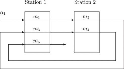
Each buffer is assumed to have infinite capacity. Following Harrison (1988), we adopt the notion of job classes. A job belongs to class k if it is either processing in step k or waiting in buffer k. We use the terms “class” and “buffer” interchangeably, with the understanding that a job in step k processing still belongs to buffer k. Let $m_k{T}_{s,k}(i)$ be the processing time of the ith class k job and let $\{m_k{T}_{s,k}(i),i\ge 1\}$ be the corresponding sequence of processing times. We assume that the elements of this sequence are independent and identically distributed (i.i.d.) with mean m_k and $\mathbb{E}[T_{s,k}(i)]=1$. The interarrival times $\{(1/{\lambda }_1)T_{e,1}(i),i\ge 1\}$ of the exogenous arrival process are assumed to be i.i.d. with mean $1/{\lambda }_1$ and $\mathbb{E}[T_{e,1}(i)]=1$. We assume these sequences are defined on a probability space $(\mathrm{\Omega },\mathcal{F},\mathbb{P})$. We also assume that different i.i.d. sequences are independent. For a positive random variable U, its squared coefficient of variation (SCV), denoted as $c^2(U)$, is defined to be

When server 1 completes the processing of a class $k\in \{1,3,5\}$ job, it needs a service discipline to decide which buffer the next job should be picked from. For our pilot example, we specify service discipline by the following list:

This list means that, at station 1, this discipline gives the highest priority to class 5, the next priority to class 3, and the lowest priority to class 1, whereas at station 2, the highest priority goes to class 2 and the lowest priority to class 4. We further assume that the service discipline is preemptive-resume: When a job with a higher rank than the one currently being served arrives at the server’s station, the service of the current job is interrupted. When all jobs of higher rank are served, the interrupted service continues from where it left off. This service discipline is referred to as SBP, which is defined for a general multiclass queueing network in Section 3.

2.2. Markov Process and Its Stability

For $t\ge 0$ define

where $Z_k(t)$ is the number of class k jobs at time t, including possibly the one in service, $U_1(t)$ is the remaining interarrival time of the next class 1 job, and $V_k(t)$ is the remaining service time of the leading class k job at time t, assuming that the class k server devotes its entire service capacity to this job. If there is no class k job in service at time t, then $V_k(t)$ is the service time of the next class k job in service.

In this paper all vectors as column vectors, but, notationally, column vectors are bulkier than row vectors. Although we could write

keeping track of all the transpose scripts ^T is also cumbersome. Therefore, going forward we omit the script ^T and envision vectors to be column vectors, unless we state otherwise. For example, we write $X(t)=(Z(t),U_1(t),V(t))$ to denote the column vector in (2.2).

It is known that $\{X(t),t\ge 0\}$ is a continuous-time Markov process with state space $S={\mathbb{Z}}_{+}^5\times {\mathbb{R}}_{+}^6$, where ${\mathbb{Z}}_{+}=\{0,1,\dots \}$, and we call X(t) the state of the queueing network at time t. This process is piecewise deterministic because between jumps, X(t) evolves deterministically in t. We adopt the convention that each sample path of the state process is right continuous.

It follows from theorem 4.1 of Dai (1995) and section 8.7 of Dai and Harrison (2020) that, under a mild assumption on the interarrival time distribution, the Markov process $\{X(t),t\ge 0\}$ is positive Harris recurrent and thus has a unique stationary distribution when the conditions

are satisfied. In such a case, we useto denote the random vector distributed according to the stationary distribution.

Lemma 2.1.

When Conditions (2.3)–(2.5) are satisfied, the following are satisfied:

$${\beta }_1\equiv \mathbb{P}\{Z_1=0,Z_3=0,Z_5=0\}=1-{\lambda }_1(m_1+m_3+m_5)=1-{\rho }_1,$$(2.6)

$${\beta }_3\equiv \mathbb{P}\{Z_3=0,Z_5=0\}=1-{\lambda }_1(m_3+m_5),\hspace{1em}{\beta }_5\equiv \mathbb{P}\{Z_5=0\}=1-{\lambda }_1{m}_5,$$(2.7)

$${\beta }_4\equiv \mathbb{P}\{Z_2=0,Z_4=0\}=1-{\lambda }_1(m_2+m_4)=1-{\rho }_2,\hspace{1em}{\beta }_2\equiv \mathbb{P}\{Z_2=0\}=1-{\lambda }_1{m}_2.$$(2.8)

For a proof of this lemma, see Lemma 6.6 in Section 6.2. Thus, when (2.3)–(2.5) hold, the quantity ρ_i is the long-run utilization of server $i\in \{1,2\}$. Conditions (2.3) and (2.4) ensure that servers 1 and 2 are not overloaded in the long run. Condition (2.5) is known as the virtual station condition, where ρ_v is the traffic intensity of the virtual station and is unusual. As explained in Dai and Vande Vate (2000), under the SBP discipline (2.1), classes 2 and 5 form a virtual station for which Condition (2.5) is the load condition. When the Markov process has a stationary distribution, we call the queueing network stable. For a general queueing network (to be introduced in Section 3) operating under an arbitrary SBP discipline, characterizing its stability region in a manner similar to (2.3)–(2.5) remains an open problem.

2.3. Heavy-Traffic Limit Theorem

We consider a sequence of queueing networks indexed by $r\in (0,1]$. Readers are referred to Section 3 for a motivation for studying a sequence of networks. For notational simplicity, only the arrival rate ${\lambda }_1^{(r)}$ is assumed to depend on r. We assume that ${\lambda }_1^{(r)}=1-r$ for $r\in (0,1]$ and that

Under Condition (2.9), (2.10) is equivalent to

Under Condition (2.9), ${\rho }_1^{(r)}={\rho }_2^{(r)}=1-r$. Thus,

In particular, ${\rho }_i^{(r)}\uparrow 1$ for i = 1, 2, as $r\to 0$. Condition (2.12) is a special case of the heavy-traffic Condition (5.4)–(5.6) to be introduced in Section 5 for a general sequence of networks. Condition (2.10) implies stability of the queueing network for any $r\in (0,1)$, and we let $X^{(r)}$ denote the random element having the stationary distribution of the Markov process $\{X^{(r)}(t),t\ge 0\}$. We let

be the column vector of steady-state job counts. The following proposition is a special case of Theorem 5.1 in Section 5. The SRBM in the proposition has been well studied; see, for example, section 2.3 of Braverman et al. (2017). To make this paper as self-contained as possible, the background materials on SRBM will be presented in Section 4.

Proposition 2.1.

There exists a random element $(Z_1^{*},Z_4^{*})\in {\mathbb{R}}_{+}^2$ such that

$$r{Z}^{(r)}\Rightarrow Z^{*}={(Z_1^{*},0,0,Z_4^{*},0)}^T,\hspace{1em} as r\to 0,$$(2.13)

where “$\Rightarrow$” denotes convergence in distribution. Furthermore, the distribution of $(Z_1^{*},Z_4^{*})$ on ${\mathbb{R}}_{+}^2$ is the unique stationary distribution of a semimartingale reflecting Brownian motion (SRBM) with covariance matrix Σ, reflection matrix R, and drift vector −Rb, where

$$\mathrm{\Sigma }=\left(\begin{array}{cc}{\mathrm{\Sigma }}_{11}& {\mathrm{\Sigma }}_{14}\\ {\mathrm{\Sigma }}_{41}& {\mathrm{\Sigma }}_{44}\end{array}\right),\hspace{1em}R=\left(\begin{array}{cc}{R}_{11}& R_{14}\\ R_{41}& R_{44}\end{array}\right)=\frac{1}{m_4-m_5}\left(\begin{array}{cc}{m}_4& -m_5\\ -1& 1\end{array}\right),\hspace{1em}b=\left(\begin{array}{c}{b}_1\\ b_4\end{array}\right)=\left(\begin{array}{c}1\\ 1\end{array}\right),$$(2.14)

and

$${\mathrm{\Sigma }}_{11}=\frac{1}{2{({\mu }_5-{\mu }_4)}^2}({({\mu }_5-{\mu }_4)}^2{c}_{e,1}^2+m_1^2{\mu }_5^2{c}_{s,1}^2+{({\mu }_4-1)}^2{c}_{s,2}^2+m_3^2{\mu }_5^2{c}_{s,3}^2+c_{s,4}^2+c_{s,5}^2),$$(2.15)

$${\mathrm{\Sigma }}_{14}={\mathrm{\Sigma }}_{41}=\frac{-1}{{({\mu }_5-{\mu }_4)}^2}(m_1^2{\mu }_5^2{\mu }_4{c}_{s,1}^2+{({\mu }_4-1)}^2{\mu }_5{c}_{s,2}^2+m_3^2{\mu }_5^2{\mu }_4{c}_{s,3}^2+{\mu }_5{c}_{s,4}^2+{\mu }_4{c}_{s,5}^2),$$(2.16)

$${\mathrm{\Sigma }}_{44}=\frac{1}{2{({\mu }_5-{\mu }_4)}^2}(m_1^2{\mu }_5^2{\mu }_4^2{c}_{s,1}^2+{({\mu }_4-1)}^2{\mu }_5^2{c}_{s,2}^2+m_3^2{\mu }_5^2{\mu }_4^2{c}_{s,3}^2+{\mu }_5^2{c}_{s,4}^2+{\mu }_4^2{c}_{s,5}^2).$$(2.17)

The remainder of this section is dedicated to proving the proposition, first for the case when interarrival and service-time distributions are exponential and then for the case when interarrival and service time distributions are general with bounded support.

2.4. Exponential Distributions

In this section, we prove Proposition 2.1, under the assumption that interarrival and service-time distributions are exponential. In such a case, we can drop the components $(U_1^{(r)}(t),V^{(r)}(t))$ in the state description $X^{(r)}(t)$ because $\{Z^{(r)}(t),t\ge 0\}$ is a CTMC on the state space $S={\mathbb{Z}}_{+}^5$, where ${\mathbb{Z}}_{+}=\{0,1,\dots \}$. When ${\lambda }_1^{(r)}=1-r$ and (2.9)–(2.10) are satisfied, each CTMC in the sequence has a unique stationary distribution, and we recall that $Z^{(r)}\in {\mathbb{Z}}_{+}^5$ denotes the steady-state job count.

2.4.1. BAR.

For the moment, we focus on a single network within the sequence of networks. We omit the index r for convenience; for example, ${\lambda }_1^{(r)}$ is denoted by λ₁. The main purpose of this section is to derive the Laplace transform version of the BAR (2.27). We use the terminology “Laplace transform” for a moment-generating function (MGF) if its domain is nonpositive.

It is well known that the stationary distribution π of the CTMC is characterized by the basic adjoint relationship (BAR)

where for each state $z\in S$ and each function $f:S\to \mathbb{R}$,and $e^{(j)}\in {\mathbb{R}}^5$ is the vector with a one in the jth component and zeros elsewhere. For a proof of (2.18), see, for example, Glynn and Zeevi (2008). When all states in S are linearly ordered, each test function $f:S\to \mathbb{R}$ is equivalent to a column vector of infinite dimensions and Gf is the usual matrix-vector product, where G is the corresponding square matrix known as the generator matrix of the CTMC.

The term

represents the state transition from state z to state $z-e^{(3)}+e^{(4)}$ due to the service completion of a class 3 job by server 1. Because of the SBP discipline in (2.1), this can happen only when class 5 has no job and class 3 has jobs. Hence, the term has the indicator function of the set $(z_5=0,z_3>0)$. The service completion triggers a deletion of a job in class 3 (the $-e^{(3)}$ term) and an addition of a job to class 4 (the $+e^{(4)}$ term). The μ₃ term reflects the service rate when server 1 is fully dedicated to a class 3 job. Other terms in the definition of Gf can be understood similarly.

Equation (2.18) is a shorthand for

The latter sum is equal to $\pi Gf$ when the stationary distribution π is viewed as a row vector, G as a square matrix, and f as a column vector. Clearly, $\pi Gf=0$ for each bounded $f:S\to \mathbb{R}$ is equivalent to

which is known as the balance equations that characterize the stationary distribution π of a CTMC with generator G.

Throughout this paper, we use the following notion. For each integer d > 0, let

Fixing a $\theta \in {\mathbb{R}}_{-}^5$, we define the bounded test function $g_{\theta }:S\to \mathbb{R}$ by

where for $a,b\in {\mathbb{R}}^5,〈a,b〉={\sum }_{k=1}^5{a}_k{b}_k$. Applying G to this function, one has

Here,

It follows from the BAR (2.18) and (2.21) that

We call this the Laplace transform version of the BAR (2.18). Let us define

The following lemma rewrites (2.23) in a more convenient form. Namely, (2.23) is written as a linear combination form of $\varphi (\theta )$ and $\varphi (\theta )-{\varphi }_i(\theta )$ for $i=1,2,\dots 5$.

Lemma 2.2.

For each $\theta \in {\mathbb{R}}_{-}^5$,

$$\begin{array}{ll}\hfill & ({\lambda }_1{\eta }_1({\theta }_1)+{\displaystyle \sum _{k=1}^5{\lambda }_1}{\xi }_k(\theta ))\varphi (\theta )+[{\mu }_5{\xi }_5(\theta )-{\mu }_3{\xi }_3(\theta )]{\beta }_5(\varphi (\theta )-{\varphi }_5(\theta ))\hfill \\ \hfill & +[{\mu }_3{\xi }_3(\theta )-{\mu }_1{\xi }_1(\theta )]{\beta }_3(\varphi (\theta )-{\varphi }_3(\theta ))+{\mu }_1{\xi }_1(\theta )(1-{\rho }_1)(\varphi (\theta )-{\varphi }_1(\theta ))\hfill \\ \hfill & +{\mu }_4{\xi }_4(\theta )(1-{\rho }_2)(\varphi (\theta )-{\varphi }_4(\theta ))+[{\mu }_2{\xi }_2(\theta )-{\mu }_4{\xi }_4(\theta )]{\beta }_2(\varphi (\theta )-{\varphi }_2(\theta ))=0,\hfill \end{array}$$(2.27)

where β_k, defined in Lemma 2.1, is the steady-state probability that all classes with priority greater or equal to class k have no customers.

Proof.

Our starting point is (2.23). Consider the last line in (2.23). Lemma 2.1 implies that

$$\begin{array}{ll}\hfill & \mathbb{E}[g_{\theta }(Z)1(Z_2>0)]=\mathbb{E}[g_{\theta }(Z)]-\mathbb{E}[g_{\theta }(Z)1(Z_2=0)]=\varphi (\theta )-{\beta }_2{\varphi }_2(\theta ),\hfill \\ \hfill & \mathbb{E}[g_{\theta }(Z)1(Z_2=0,Z_4>0)]={\beta }_2{\varphi }_2(\theta )-{\beta }_4{\varphi }_4(\theta ).\hfill \end{array}$$

Hence,

$$\begin{array}{l}\mathbb{E}[({\mu }_2{\xi }_2(\theta )1(Z_2>0)+{\mu }_4{\xi }_4(\theta )1(Z_2=0,Z_4>0))g_{\theta }(Z)]\hfill \\ ={\mu }_2{\xi }_2(\theta )\varphi (\theta )+[{\mu }_2{\xi }_2(\theta )-{\mu }_4{\xi }_4(\theta )]{\beta }_2(-{\varphi }_2(\theta ))+{\mu }_4{\xi }_4(\theta ){\beta }_4(-{\varphi }_4(\theta ))\hfill \\ =({\mu }_2{\xi }_2(\theta )-[{\mu }_2{\xi }_2(\theta )-{\mu }_4{\xi }_4(\theta )]{\beta }_2-{\mu }_4{\xi }_4(\theta ){\beta }_4)\varphi (\theta )\hfill \\ +[{\mu }_2{\xi }_2(\theta )-{\mu }_4{\xi }_4(\theta )]{\beta }_2(\varphi (\theta )-{\varphi }_2(\theta ))+{\mu }_4{\xi }_4(\theta ){\beta }_4(\varphi (\theta )-{\varphi }_4(\theta ))\hfill \\ =({\mu }_2{\xi }_2(\theta )(1-{\beta }_2)+{\mu }_4{\xi }_4(\theta )({\beta }_2-{\beta }_4))\varphi (\theta )\hfill \\ +[{\mu }_2{\xi }_2(\theta )-{\mu }_4{\xi }_4(\theta )]{\beta }_2(\varphi (\theta )-{\varphi }_2(\theta ))+{\mu }_4{\xi }_4(\theta ){\beta }_4(\varphi (\theta )-{\varphi }_4(\theta )).\hfill \end{array}$$

From Lemma 2.1, we know that ${\beta }_4=1-{\lambda }_1(m_2+m_4)=1-{\rho }_2$ and ${\beta }_2=1-{\lambda }_1{m}_2$, implying that the right-hand side equals

$$\begin{array}{l}({\lambda }_1{\xi }_2(\theta )+{\lambda }_1{\xi }_4(\theta ))\varphi (\theta )\hfill \\ +[{\mu }_2{\xi }_2(\theta )-{\mu }_4{\xi }_4(\theta )]{\beta }_2(\varphi (\theta )-{\varphi }_2(\theta ))+{\mu }_4{\xi }_4(\theta )(1-{\rho }_2)(\varphi (\theta )-{\varphi }_4(\theta )).\hfill \end{array}$$(2.28)

Similarly, one can show that

$$\begin{array}{l}\mathbb{E}[({\mu }_5{\xi }_5(\theta )1(Z_5>0)+{\mu }_3{\xi }_3(\theta )1(Z_3>0,Z_5=0)+{\mu }_1{\xi }_1(\theta )1(Z_1>0,Z_3=0,Z_5=0))g_{\theta }(Z)]\hfill \\ =({\lambda }_1{\xi }_1(\theta )+{\lambda }_1{\xi }_3(\theta )+{\lambda }_1{\xi }_5(\theta ))\varphi (\theta )+[{\mu }_5{\xi }_5(\theta )-{\mu }_3{\xi }_3(\theta )]{\beta }_5(\varphi (\theta )-{\varphi }_5(\theta ))\hfill \\ +[{\mu }_3{\xi }_3(\theta )-{\mu }_1{\xi }_1(\theta )]{\beta }_3(\varphi (\theta )-{\varphi }_3(\theta ))+{\mu }_1{\xi }_1(\theta )(1-{\rho }_1)(\varphi (\theta )-{\varphi }_1(\theta )).\hfill \end{array}$$(2.29)

Finally, (2.27) follows from (2.23) and the expressions in (2.28) and (2.29). □

2.4.2. Taylor Expansion and Asymptotic BAR.

For each $\theta \in {\mathbb{R}}_{-}^5$, define

which is analogous to the definition of $\varphi (\theta )$ in (2.24). Define ${\varphi }_k^{(r)}(\theta )$ similarly for $k\in \{1,\dots ,5\}$. We now present Lemma 2.3, in which we start with (2.27) and replace ${\eta }_1({\theta }_1)$ and ${\xi }_k(\theta )$ by their second-order Taylor expansions, which are simpler to work with, to derive what we call the asymptotic BAR in (2.34). Later we will see how the asymptotic BAR allows us to characterize the limiting distribution of $r{Z}^{(r)}$ as $r\to 0$.

To state Lemma 2.3, we define

We will see in the proof of Lemma 2.3 that ${\overline{\eta }}_1({\theta }_1)$ and ${\tilde{\eta }}_1({\theta }_1)$ are the first- and second-order terms, respectively, of the Taylor expansion of ${\eta }_1({\theta }_1)$. Similarly, we define

Last, we define

to be the second-order approximations of ${\eta }_1({\theta }_1)$ and ${\xi }_k(\theta )$, respectively.

Lemma 2.3.

For each $\theta \in {\mathbb{R}}_{-}^5$, as $r\to 0$,

$$\begin{array}{ll}\hfill & r^2({\lambda }_1^{(r)}{\tilde{\eta }}_1({\theta }_1)+{\displaystyle \sum _{k=1}^5{\lambda }_1^{(r)}}\widetilde{{\xi }_k}(\theta )){\varphi }^{(r)}(\theta )\hfill \\ \hfill & \hspace{1em}+r^2{\mu }_1{\overline{\xi }}_1(\theta )({\varphi }^{(r)}(\theta )-{\varphi }_1^{(r)}(\theta ))+{\mu }_4{r}^2{\overline{\xi }}_4(\theta )({\varphi }^{(r)}(\theta )-{\varphi }_4^{(r)}(\theta ))\hfill \\ \hfill & \hspace{1em}+[{\mu }_3{\xi }_3^{*}(r\theta )-{\mu }_1{\xi }_1^{*}(r\theta )]{\beta }_3^{(r)}({\varphi }^{(r)}(\theta )-{\varphi }_3^{(r)}(\theta ))\hfill \\ \hfill & \hspace{1em}+[{\mu }_5{\xi }_5^{*}(r\theta )-{\mu }_3{\xi }_3^{*}(r\theta )]{\beta }_5^{(r)}({\varphi }^{(r)}(\theta )-{\varphi }_5^{(r)}(\theta ))\hfill \\ \hfill & \hspace{1em}+[{\mu }_2{\xi }_2^{*}(r\theta )-{\mu }_4{\xi }_4^{*}(r\theta )]{\beta }_2^{(r)}({\varphi }^{(r)}(\theta )-{\varphi }_2^{(r)}(\theta ))=o(r^2).\hfill \end{array}$$(2.34)

Proof.

Replacing θ in (2.27) by $r\theta$, one has that for each $\theta \in {\mathbb{R}}_{-}^5$ and each $r\in (0,1)$,

$$\begin{array}{ll}\hfill & ({\lambda }_1^{(r)}{\eta }_1(r{\theta }_1)+{\displaystyle \sum _{k=1}^5{\lambda }_1^{(r)}}{\xi }_k(r\theta )){\varphi }^{(r)}(\theta )+[{\mu }_5{\xi }_5(r\theta )-{\mu }_3{\xi }_3(r\theta )]{\beta }_5^{(r)}({\varphi }^{(r)}(\theta )-{\varphi }_5^{(r)}(\theta ))\hfill \\ \hfill & +[{\mu }_3{\xi }_3(r\theta )-{\mu }_1{\xi }_1(r\theta )]{\beta }_3^{(r)}({\varphi }^{(r)}(\theta )-{\varphi }_3^{(r)}(\theta ))+{\mu }_1{\xi }_1(r\theta )(1-{\rho }_1^{(r)})({\varphi }^{(r)}(\theta )-{\varphi }_1^{(r)}(\theta ))\hfill \\ \hfill & +{\mu }_4{\xi }_4(r\theta )(1-{\rho }_2^{(r)})({\varphi }^{(r)}(\theta )-{\varphi }_4^{(r)}(\theta ))+[{\mu }_2{\xi }_2(r\theta )-{\mu }_4{\xi }_4(r\theta )]{\beta }_2^{(r)}({\varphi }^{(r)}(\theta )-{\varphi }_2^{(r)}(\theta ))=0.\hfill \end{array}$$

Using the Taylor expansion $e^x=1+x+\frac{1}{2}{x}^2+o(x)$ when $x\to 0$, one has

$${\eta }_1({\theta }_1)={\eta }_1^{*}({\theta }_1)+o({\theta }_1^2) \text{as} {\theta }_1\to 0,$$(2.35)

$${\xi }_k(\theta )={\xi }_k^{*}(\theta )+o(|\theta {|}^2) \text{as} \theta \to 0 \text{for} k\in \{1,\dots ,5\}.$$(2.36)

Therefore, for each $\theta \in {\mathbb{R}}_{-}^5$ as $r\to 0$,

$$\begin{array}{ll}\hfill & ({\lambda }_1^{(r)}{\eta }_1^{*}(r{\theta }_1)+{\displaystyle \sum _{k=1}^5{\lambda }_1^{(r)}}{\xi }_k^{*}(r\theta )){\varphi }^{(r)}(\theta )+[{\mu }_5{\xi }_5^{*}(r\theta )-{\mu }_3{\xi }_3^{*}(r\theta )]{\beta }_5^{(r)}({\varphi }^{(r)}(\theta )-{\varphi }_5^{(r)}(\theta ))\hfill \\ \hfill & +[{\mu }_3{\xi }_3^{*}(r\theta )-{\mu }_1{\xi }_1^{*}(r\theta )]{\beta }_3^{(r)}({\varphi }^{(r)}(\theta )-{\varphi }_3^{(r)}(\theta ))+{\mu }_1{\xi }_1^{*}(r\theta )(1-{\rho }_1^{(r)})({\varphi }^{(r)}(\theta )-{\varphi }_1^{(r)}(\theta ))\hfill \\ \hfill & +{\mu }_4{\xi }_4^{*}(r\theta )(1-{\rho }_2^{(r)})({\varphi }^{(r)}(\theta )-{\varphi }_4^{(r)}(\theta ))+[{\mu }_2{\xi }_2^{*}(r\theta )-{\mu }_4{\xi }_4^{*}(r\theta )]{\beta }_2^{(r)}({\varphi }^{(r)}(\theta )-{\varphi }_2^{(r)}(\theta ))=o(r^2).\hfill \end{array}$$

Using the facts that ${\overline{\eta }}_1({\theta }_1)+{\sum }_{k=1}^5{\overline{\xi }}_k(\theta )=0$, that ${\tilde{\xi }}_k(r\theta )=r^2{\tilde{\xi }}_k(\theta )$ for each $\theta \in {\mathbb{R}}_{-}^5$, and that $1-{\rho }_i^{(r)}=r$, we have (2.34), proving the lemma. □

2.4.3. SSC.

It follows from theorem 3.7 and section 4.1 of Cao et al. (2022) that the following moment SSC holds:

In fact, we now argue that as a consequence of (2.37), for any $\theta \in {\mathbb{R}}_{-}^5$,

where, for a function $f:{\mathbb{R}}^5\to \mathbb{R},\hspace{0.17em}f({\theta }_L,0)$ is a shorthand for $f({\theta }_1,0,0,{\theta }_4,0)$ with ${\theta }_L={({\theta }_1,{\theta }_4)}^T$. We refer to (2.38) as the Laplace transform version of SSC. To prove the first equality in (2.38),where the second inequality follows from $1-e^{-x}\le x$ for $x\ge 0$. The last term converges to zero because of (2.37) and Jensen’s inequality. The rest of (2.38) is proved similarly.

Proof of Proposition 2.1.

The SSC in the preceding paragraph implies that ${\lim }_{r\to 0}r{Z}_k^{(r)}\Rightarrow 0$ for $k\in \{2,3,5\}$. To prove Proposition 2.1, it remains to show that $(r{Z}_1^{(r)},r{Z}_4^{(r)})$ converges and characterizes the limit. We begin with the following lemma, which is stated for the general queueing network setting in Lemma 7.1.

Lemma 2.4.

For any sequence ${\{({\varphi }^{(r_n)}(\theta ),{\varphi }_1^{(r_n)}(\theta ),\dots ,{\varphi }_5^{(r_n)}(\theta ))\}}_{n=1}^{\infty }$ with $r_n\in (0,1)$ and ${\lim }_{n\to \infty }{r}_n=0$, there exists a subsequence indexed by $\{r_{n_k}\}$ such that

$$\underset{k\to \infty }{\lim }({\varphi }^{(r_{n_k})}(\theta ),{\varphi }_1^{(r_{n_k})}(\theta ),\dots ,{\varphi }_5^{(r_{n_k})}(\theta ))=({\varphi }^{*}(\theta ),{\varphi }_1^{*}(\theta ),\dots ,{\varphi }_5^{*}(\theta ))\hspace{1em} \mathit{\text{for}} \mathit{\text{each}} \theta \in {\mathbb{R}}_{-}^5.$$

We call $({\varphi }^{*}(\theta ),{\varphi }_1^{*}(\theta ),\dots ,{\varphi }_5^{*}(\theta ))$ a limit point of ${\{({\varphi }^{(r)}(\theta ),{\varphi }_1^{(r)}(\theta ),\dots ,{\varphi }_5^{(r)}(\theta ))\}}_{r\in (0,1)}$.

We show that the set of all limit points in Lemma 2.4 is a singleton by proving that there is a random vector $(Z_1^{*},Z_4^{*})\in {\mathbb{R}}_{+}^2$, independent of the subsequence $\{r_{n_k}\}$, such that

Because every sequence ${\{{\varphi }^{(r_n)}(\theta )\}}_{n=1}^{\infty }$ contains a convergent subsequence that converges to the limit point defined by (2.39), it follows that

which is equivalent to the convergence in (2.13). The following informal discussion outlines how we prove (2.39).

Let us assume for simplicity that ${\varphi }^{(r)}(\theta ),{\varphi }_1^{(r)}(\theta ),\dots ,{\varphi }_5^{(r)}(\theta )$ converge pointwise as $r\to 0$. Otherwise, we can replace r by $r_{n_k}$ and be assured that ${\varphi }^{(r_{n_k})}(\theta ),{\varphi }_1^{(r_{n_k})}(\theta ),\dots ,{\varphi }_5^{(r_{n_k})}(\theta )$ converge. We characterize the limit point using the asymptotic BAR (2.34) as follows. Dividing both sides of (2.34) by r² and letting $r\to 0$ yields

We proceed in two steps. In step one, we identify a subset of ${\mathbb{R}}_{-}^5$ such that the right-hand side of (2.40) is zero for all θ in this subset. We do this because we are unable to characterize the right-hand side outside this subset. Step 1 requires Lemmas 2.5, 2.6, and 2.7, which are stated later. Following these lemmas, we use (2.40), the right-hand side of which now equals zero, to characterize ${\varphi }^{*}(\theta )$ and prove (2.39)—this is step 2.

Let us compare our example to Braverman et al. (2017), who applied the BAR approach with Laplace transforms to generalized Jackson networks (GJNs). In that paper, the authors derived an asymptotic BAR for GJNs, which allowed them to obtain an equation that is analogous to (2.40). However, because GJNs are single-class queueing networks, the right-hand side of their equation equals zero. This means that Braverman et al. (2017) did not need to perform step one of the previous paragraph, whereas we do because our two-station example is a multiclass queueing network.

We now carry out step 1. To understand how to choose θ so the right-hand side of (2.40) equals zero, we examine the first term inside the parentheses. Namely,

Because ${\overline{\xi }}_k(\theta )$ are linear in θ, we show in Lemma 2.5 that we can choose θ to make the first term on the right-hand side equal zero. Furthermore, ${\sup }_{r\in (0,1)}|{\tilde{\xi }}_k(r\theta )|/r^2<\infty$ because ${\tilde{\xi }}_k(\theta )$ are quadratic in θ; see (2.31). Therefore, to prove that the second term vanishes as $r\to 0$, we show in Lemma 2.6 that ${\lim }_{r\to 0}({\varphi }^{(r)}(\theta )-{\varphi }_k^{(r)}(\theta ))=0$ for $k\in \{2,3,5\}$.

Recall that all vectors are envisioned as column vectors, and recall our convention of writing column vectors discussed in Section 2.2.

Lemma 2.5.

Recall the definition of ${\overline{\xi }}_k(\theta )$ from (2.31) and consider the system of linear equations:

$${\mu }_3{\overline{\xi }}_3(\theta )-{\mu }_1{\overline{\xi }}_1(\theta )={\mu }_3({\theta }_4-{\theta }_3)-{\mu }_1({\theta }_2-{\theta }_1)=0,$$(2.41)

$${\mu }_5{\overline{\xi }}_5(\theta )-{\mu }_3{\overline{\xi }}_3(\theta )=-{\mu }_5{\theta }_5-{\mu }_3({\theta }_4-{\theta }_3)=0,$$(2.42)

$${\mu }_2{\overline{\xi }}_2(\theta )-{\mu }_4{\overline{\xi }}_4(\theta )={\mu }_2({\theta }_3-{\theta }_2)-{\mu }_4({\theta }_5-{\theta }_4)=0.$$(2.43)

For each fixed ${\theta }_L=({\theta }_1,{\theta }_4)\in {\mathbb{R}}^2$, there exists a unique $h({\theta }_L)=({\theta }_2,{\theta }_3,{\theta }_5)$ such that $\theta =({\theta }_1,{\theta }_2,{\theta }_3,{\theta }_4,{\theta }_5)$ satisfies (2.41)–(2.43). Furthermore, the set Θ_L, defined as

$${\mathrm{\Theta }}_L=\{({\theta }_1,{\theta }_4)\in {\mathbb{R}}_{-}^2:m_4-\frac{{\mu }_5{m}_4-1}{m_1{\mu }_5}<\frac{{\theta }_4}{{\theta }_1}<m_4\},$$(2.44)

is a nonempty and open set, and

$$h({\theta }_L)=({\theta }_2,{\theta }_3,{\theta }_5)<0\hspace{1em} \mathit{\text{for}} \mathit{\text{all}} \hspace{1em}{\theta }_L=({\theta }_1,{\theta }_4)\in {\mathrm{\Theta }}_L.$$(2.45)

Proof.

Fix a ${\theta }_L=({\theta }_1,{\theta }_4)\in {\mathbb{R}}^2$. One can verify that $\theta =({\theta }_1,{\theta }_2,{\theta }_3,{\theta }_4,{\theta }_5)$ with

$${\theta }_5=\frac{1}{{\mu }_5{m}_4-1}[m_4{\theta }_1-{\theta }_4],$$(2.46)

$${\theta }_2={\theta }_1-m_1{\mu }_5{\theta }_5,$$(2.47)

$${\theta }_3={\theta }_4+m_3{\mu }_5{\theta }_5.$$(2.48)

This satisfies Equations (2.41)–(2.43). Now for ${\theta }_L\in {\mathrm{\Theta }}_L$, we have ${\theta }_4>m_4{\theta }_1$ and ${\theta }_4<0$, which implies that ${\theta }_5<0$ and ${\theta }_3<0$. Finally, ${\theta }_2<0$ follows from $m_4-({\mu }_5{m}_4-1)/(m_1{\mu }_5)<\frac{{\theta }_4}{{\theta }_1}$ and ${\theta }_1<0$. □

Lemma 2.6.

For each $\theta \in {\mathbb{R}}_{-}^5$,

$$\underset{r\to 0}{\lim }({\varphi }^{(r)}(\theta )-{\varphi }_k^{(r)}(\theta ))=0,\hspace{1em}k\in \{2,3,5\}.$$(2.49)

Proof.

We prove the lemma for k = 2. Other cases can be proved similarly. Recalling from (2.33) that ${\xi }_k^{*}(\theta )={\overline{\xi }}_k(\theta )+{\tilde{\xi }}_k(\theta )$, it follows from (2.34) that for each $\theta \in {\mathbb{R}}_{-}^5$,

$$\begin{array}{ll}\hfill & [{\mu }_3{\overline{\xi }}_3(\theta )-{\mu }_1{\overline{\xi }}_1(\theta )]{\beta }_3^{(r)}({\varphi }^{(r)}(\theta )-{\varphi }_3^{(r)}(\theta ))+[{\mu }_5{\overline{\xi }}_5(\theta )-{\mu }_3{\overline{\xi }}_3(\theta )]{\beta }_5^{(r)}({\varphi }^{(r)}(\theta )-{\varphi }_5^{(r)}(\theta ))\hfill \\ \hfill & +[{\mu }_2{\overline{\xi }}_2(\theta )-{\mu }_4{\overline{\xi }}_4(\theta )]{\beta }_2^{(r)}({\varphi }^{(r)}(\theta )-{\varphi }_2^{(r)}(\theta ))=o(1).\hfill \end{array}$$(2.50)

For each fixed ${\theta }_L=({\theta }_1,{\theta }_4)\in {\mathbb{R}}_{-}^2$ and ${\theta }_5\in \mathbb{R}$, set θ₂ and θ₃ follows (2.47) and (2.48), respectively. One can verify that $\theta =({\theta }_1,{\theta }_2,{\theta }_3,{\theta }_4,{\theta }_5)$ satisfies (2.41) and (2.42). Furthermore, it follows from (2.46) that one can choose ${\theta }_5<0$ small enough so that ${\theta }_2<0,\hspace{0.17em}{\theta }_3<0$ and

$${\mu }_2{\overline{\xi }}_2(\theta )-{\mu }_4{\overline{\xi }}_4(\theta )\ne 0.$$(2.51)

For this choice of $\theta =({\theta }_1,{\theta }_2,{\theta }_3,{\theta }_4,{\theta }_5)$, (2.50) gives

$$\underset{r\to 0}{\lim }({\varphi }^{(r)}(\theta )-{\varphi }_2^{(r)}(\theta ))=0,$$

which, together with SSC (2.38), yields

$$\underset{r\to 0}{\lim }({\varphi }^{(r)}({\theta }_L,0)-{\varphi }_2^{(r)}({\theta }_L,0))=0\hspace{1em} \text{for} \text{each} \hspace{1em}{\theta }_L\in {\mathbb{R}}_{-}^2.$$(2.52)

Now for any $\theta \in {\mathbb{R}}_{-}^5$, Equation (2.52) and SSC (2.38) imply (2.49) for k = 2. □

Lemma 2.7.

For each ${\theta }_L\in {\mathrm{\Theta }}_L$, let $\theta =({\theta }_L,{\theta }_H)$ be the unique θ that satisfies (2.41)–(2.43). Then any limit point $({\varphi }^{*}(\theta ),{\varphi }_1^{*}(\theta ),\dots ,{\varphi }_5^{*}(\theta ))$ satisfies

$$\begin{array}{ll}0\hfill & =({\tilde{\eta }}_1({\theta }_1)+{\displaystyle \sum _{k=1}^5\widetilde{{\xi }_k}}(\theta )){\varphi }^{*}(\theta )+{\mu }_1{\overline{\xi }}_1(\theta )({\varphi }^{*}(\theta )-{\varphi }_1^{*}(\theta ))+{\mu }_4{\overline{\xi }}_4(\theta )({\varphi }^{*}(\theta )-{\varphi }_4^{*}(\theta ))\hfill \\ \hfill & =({\tilde{\eta }}_1({\theta }_1)+{\displaystyle \sum _{k=1}^5\widetilde{{\xi }_k}}(\theta )){\varphi }^{*}({\theta }_L,0)+{\mu }_1{\overline{\xi }}_1(\theta )({\varphi }^{*}({\theta }_L,0)-{\varphi }_1^{*}({\theta }_L,0))\hfill \\ \hfill & \hspace{1em}+{\mu }_4{\overline{\xi }}_4(\theta )({\varphi }^{*}({\theta }_L,0)-{\varphi }_4^{*}({\theta }_L,0)),\hspace{1em}\hspace{1em}\hspace{1em}\hspace{1em}\hspace{1em}\hspace{1em}\hspace{1em}\hspace{1em}\hspace{1em}\hspace{1em}\hspace{1em}\hspace{1em}\hspace{1em}\hspace{1em}\hspace{1em}\hspace{1em}\hspace{1em}\hspace{1em}\hspace{0.5em}\hspace{1em}{\theta }_L\in {\mathrm{\Theta }}_L.\hfill \end{array}$$(2.53)

Proof.

The first equality follows by combining Lemmas 2.5 and 2.6 with the discussion preceding Lemma 2.5. The second equality follows from the Laplace transform version of SSC (2.38). □

We now prove that for each limit point ${\varphi }^{*}$, (2.39) holds for some random vector $(Z_1^{*},Z_4^{*})$ that is independent of the subsequence that generates the limit point.

Our starting point is (2.53) in Lemma 2.7. In (2.53), for each ${\theta }_L=({\theta }_1,{\theta }_4)\in {\mathrm{\Theta }}_L$, θ is set to be the vector $({\theta }_1,{\theta }_2,{\theta }_3,{\theta }_4,{\theta }_5)$ with ${\theta }_5,{\theta }_2$, and with θ₃ being defined through (2.46)–(2.48). Observe that

where the 2 × 2 matrix R is given in (2.14), and $R^{(1)}$ and $R^{(4)}$ are the first and fourth columns of R, respectively. Also,where the second equality follows from Lemma 2.8 and ${\mathrm{\Sigma }}_{11}$, ${\mathrm{\Sigma }}_{14}$ and ${\mathrm{\Sigma }}_{44}$ are given by (2.15)–(2.17) with $c_{e,1}^2=c_{s,k}^2=1$ for $k=1,\dots ,5$; the latter is true because the interarrival and service-time distributions are exponential. Therefore, (2.53) is reduced to

Because R in (2.14) is an $\mathcal{M}$ matrix, it follows from Proposition 5.1 and the proof of (6.3) and (6.4) in Braverman et al. (2017) that ${\varphi }^{*}(0-,0,0,0-,0)=1,\hspace{0.17em}{\varphi }_1^{*}(0,0,0,0-,0)=1$, and ${\varphi }_4^{*}(0-,0,0,0,0)=1$, where

It follows that ${\varphi }^{*}({\theta }_1,0,0,{\theta }_4,0)$ is the Laplace transform of a probability measure ν on ${\mathbb{R}}_{+}^2$, ${\varphi }_1^{*}(0,0,0,{\theta }_4,0)$ is the Laplace transform of a probability measure ν₁ on ${\mathbb{R}}_{+}$, and ${\varphi }_4^{*}({\theta }_1,0,0,0,0)$ is the Laplace transform of a probability measure ν₄ on ${\mathbb{R}}_{+}$, namely

see, for example, lemma 6.1 of Braverman et al. (2017) for an argument. Furthermore, it follows from Lemma 4.1 in Section 4 that the probability measures ν, ν₁, and ν₄ are unique. If we consider θ₁ and θ₄ as complex variables, then the aforementioned Laplace transforms have analytic extensions from Θ_L to ${\mathbb{R}}_{-}^2$. Let $(Z_1^{*},Z_4^{*})$ be a random vector that has the distribution of ν. Then,where the first equality follows the Laplace version of SSC (2.38). The uniqueness of the probability measure ν proves (2.39). □

Thus, the proof of Proposition 2.1 is completed by Lemma 2.8 below, which computes ${\mathrm{\Sigma }}_{i,j}$ for $i,j=1,4$.

Lemma 2.8.

For each $({\theta }_1,{\theta }_4)\in {\mathbb{R}}^2$, let θ₂, θ₃, and θ₅ be defined through (2.46)–(2.48). Then, the quadratic equation

$$\frac{1}{2}\left(c_{e,1}^2{\theta }_1^2+{\displaystyle \sum _{k=1}^4{c}_{s,k}^2}{(-{\theta }_k+{\theta }_{k+1})}^2+c_{s,5}^2{\theta }_5^2\right)={\mathrm{\Sigma }}_{11}{\theta }_1^2+2{\mathrm{\Sigma }}_{14}{\theta }_1{\theta }_4+{\mathrm{\Sigma }}_{44}{\theta }_4^2$$(2.56)

holds for each $({\theta }_1,{\theta }_4)\in {\mathbb{R}}^2$ if and only if ${\mathrm{\Sigma }}_{11},\hspace{0.17em}{\mathrm{\Sigma }}_{14}$, and ${\mathrm{\Sigma }}_{44}$ are given by (2.15)–(2.17).

Proof.

Because ${\theta }_5=({\theta }_1-{\mu }_4{\theta }_4)/({\mu }_5-{\mu }_4)$ and $(m_1+m_3){\mu }_5={\mu }_5-1$ by $m_1+m_3+m_5=1$, quadratic terms in the left side of (2.56) are computed as

$$\begin{array}{ll}{({\theta }_2-{\theta }_1)}^2\hfill & =m_1^2{\mu }_5^2{\theta }_5^2=\frac{m_1^2{\mu }_5^2}{{({\mu }_5-{\mu }_4)}^2}{({\theta }_1-{\mu }_4{\theta }_4)}^2,\hfill \\ {({\theta }_3-{\theta }_2)}^2\hfill & ={({\theta }_4-{\theta }_1+(m_1+m_3){\mu }_5{\theta }_5)}^2={({\theta }_4-{\theta }_1+({\mu }_5-1){\theta }_5)}^2\hfill \\ \hfill & ={\left({\theta }_4-{\theta }_1+\frac{{\mu }_5-1}{{\mu }_5-{\mu }_4}({\theta }_1-{\mu }_4{\theta }_4)\right)}^2=\frac{{({\mu }_4-1)}^2}{{({\mu }_5-{\mu }_4)}^2}{({\theta }_1-{\mu }_5{\theta }_4)}^2,\hfill \\ {({\theta }_4-{\theta }_3)}^2\hfill & =\frac{m_3^2{\mu }_5^2}{{({\mu }_5-{\mu }_4)}^2}{({\theta }_1-{\mu }_4{\theta }_4)}^2,\hfill \\ {({\theta }_5-{\theta }_4)}^2\hfill & ={\left(\frac{{\theta }_1-{\mu }_4{\theta }_4}{{\mu }_5-{\mu }_4}-{\theta }_4\right)}^2=\frac{1}{{({\mu }_5-{\mu }_4)}^2}{({\theta }_1-{\mu }_5{\theta }_4)}^2,\hfill \\ {\theta }_5^2\hfill & =\frac{1}{{({\mu }_5-{\mu }_4)}^2}{({\theta }_1-{\mu }_4{\theta }_4)}^2.\hfill \end{array}$$

Hence, collecting the coefficients of ${\theta }_1^2$, we have

$$\begin{array}{ll}{\mathrm{\Sigma }}_{11}\hfill & =\frac{1}{2}(c_{e,1}^2+c_{s,1}^2\frac{m_1^2{\mu }_5^2}{{({\mu }_5-{\mu }_4)}^2}+c_{s,2}^2{\left(\frac{{\mu }_4-1}{{\mu }_5-{\mu }_4}\right)}^2\hfill \\ \hfill & \hspace{1em}\hspace{1em}+c_{s,3}^2\frac{m_3^2{\mu }_5^2}{{({\mu }_5-{\mu }_4)}^2}+c_{s,4}^2\frac{1}{{({\mu }_5-{\mu }_4)}^2}+c_{s,5}^2\frac{1}{{({\mu }_5-{\mu }_4)}^2})\hfill \\ \hfill & =\frac{1}{2{({\mu }_5-{\mu }_4)}^2}({({\mu }_5-{\mu }_4)}^2{c}_{e,1}^2+m_1^2{\mu }_5^2{c}_{s,1}^2+{({\mu }_4-1)}^2{c}_{s,2}^2+m_3^2{\mu }_5^2{c}_{s,3}^2+c_{s,4}^2+c_{s,5}^2).\hfill \end{array}$$

(2.16) and (2.17) are similarly obtained. □

2.5. General Bounded Distributions

In this section, we prove Proposition 2.1 when interarrival and service-time distributions are general. To keep our notational system simple, we further assume these distributions have bounded supports. The bounded support assumption will be replaced with a moment condition in Sections 7 and 8.

Define

where $c_{e,1}^2$ is the SCV of the interarrival time distribution, and $c_{s,k}^2$ is the SCV of the class k service-time distribution.

The main purpose of this section is to prove the following lemma.

Lemma 2.9.

Assume that interarrival and service-time distributions have bounded supports. Then Lemma 2.7 continues to hold with ${\tilde{\eta }}_1({\theta }_1)$ and ${\tilde{\xi }}_k(\theta )$ defined in (2.57) and ${\overline{\eta }}_1({\theta }_1)$ and ${\overline{\xi }}_k(\theta )$ defined in (2.30) and (2.31).

Once Lemma 2.9 is proved, the remaining steps in the proof of Proposition 2.1 for the general distribution case are the same as for the exponential case. To prove Lemma 2.9, we define, for each $\theta \in {\mathbb{R}}^5,\hspace{0.17em}{\eta }_1({\theta }_1)$ and ${\xi }_k(\theta )$ as the solutions to

We intentionally reuse the notation ${\eta }_1(\theta )$ and ${\xi }_k(\theta )$ from (2.22). This causes no harm because these two sets of definitions are identical when $T_{e,1}$ and $T_{s,k}$ are exponentially distributed. It is proved in Braverman et al. (2017) that when $T_{e,1}$ and $T_{s,k}$ have bounded support, then ${\eta }_1({\theta }_1)$ and ${\xi }_k(\theta )$ are well defined for each $\theta \in {\mathbb{R}}_{-}^5$. Furthermore, the following lemma holds.

Lemma 2.10.

Taylor expansions (2.35)–(2.36) continue to hold with ${\tilde{\eta }}_1({\theta }_1)$ and ${\tilde{\xi }}_k(\theta )$ defined in (2.57).

Recall that we assume the sequence of two-station, five-class networks has arrival rates ${\lambda }_1^{(r)}=1-r$ and mean service times satisfying (2.9) and (2.10). Let $\kappa >0$ be the constant such that the support of each distribution is contained in the interval $[0,\kappa ]$. Recall that $X^{(r)}$ is the random vector representing the unique stationary distribution on $S\equiv {\mathbb{Z}}_{+}^5\times {[0,\kappa ]}^6$ of the corresponding Markov process. In the following, we use

to denote a generic state. For each $\theta \in {\mathbb{R}}_{-}^5$, define

For each fixed $\theta \in {\mathbb{R}}_{-}^5$, it is clear that $f_{\theta }(x)$ is a bounded function of $x\in S$. For each $\theta \in {\mathbb{R}}_{-}^5$, define

Lemma 2.9 follows immediately from the following two lemmas.

Lemma 2.11.

For each ${\theta }_L\in {\mathrm{\Theta }}_L$, let $\theta =({\theta }_L,{\theta }_H)$ be the unique θ that satisfies (2.41)–(2.43). Then, any limit point $({\psi }^{*}(\theta ),{\psi }_1^{*}(\theta ),\dots ,{\psi }_5^{*}(\theta ))$ of ${\{({\psi }^{(r)}(\theta ),{\psi }_1^{(r)}(\theta ),\dots ,{\psi }_5^{(r)}(\theta ))\}}_{r\in (0,1)}$ satisfies

$$({\tilde{\eta }}_1({\theta }_1)+{\displaystyle \sum _{k=1}^5\widetilde{{\xi }_k}}(\theta )){\psi }^{*}(\theta )+{\mu }_1{\overline{\xi }}_1(\theta )({\psi }^{*}(\theta )-{\psi }_1^{*}(\theta ))+{\mu }_4{\overline{\xi }}_4(\theta )({\psi }^{*}(\theta )-{\psi }_4^{*}(\theta ))=0,$$

where ${\tilde{\eta }}_1({\theta }_1)$ and ${\tilde{\xi }}_k(\theta )$ are defined in (2.57) and ${\overline{\xi }}_k(\theta )$ is defined in (2.31).

This lemma is similar to Lemma 2.7, with ${\psi }^{(r)}(\theta )$ replacing ${\varphi }^{(r)}(\theta )$. The proof of Lemma 2.11 will be at the end of this section after we introduce the BAR for $X^{(r)}$. The following lemma allows one to derive Lemma 2.7 from Lemma 2.11 immediately.

Lemma 2.12.

For each $\theta \in {\mathbb{R}}_{-}^5$, as $r\to 0$,

$${\varphi }^{(r)}(\theta )-{\psi }^{(r)}(\theta )=o(1)\hspace{1em} \mathit{\text{and}} \hspace{1em}{\varphi }_k^{(r)}(\theta )-{\psi }_k^{(r)}(\theta )=o(1).$$

Proof.

Fix a $\theta \in {\mathbb{R}}_{-}^5$. For each $x\in S$ and each $r\in (0,1)$,

$$\begin{array}{ll}|g_{r\theta }(z)-f_{r\theta }(x)|\hfill & =g_{r\theta }(z)\left|1-\exp (-{\lambda }_1^{(r)}{\eta }_1(r{\theta }_1)u_1-{\displaystyle \sum _{k=1}^5{\mu }_k}{\xi }_k(r\theta )v_k)\right|\hfill \\ \hfill & \le e^{|\mathrm{\Lambda }(r,\theta ,u_1,v)|}|\mathrm{\Lambda }(r,\theta ,u_1,v)|\le e^{\mathrm{\Lambda }(r\theta )}\mathrm{\Lambda }(r\theta ),\hfill \end{array}$$

where

$$\begin{array}{ll}\hfill & \mathrm{\Lambda }(r,\theta ,u_1,v)\equiv -{\lambda }_1^{(r)}{\eta }_1(r{\theta }_1)u_1-{\displaystyle \sum _{k=1}^5{\mu }_k}{\xi }_k(r\theta )v_k,\hfill \\ \hfill & \mathrm{\Lambda }(\theta )\equiv \kappa |{\eta }_1({\theta }_1)|+{\displaystyle \sum _{k=1}^5\kappa }{\mu }_k|{\xi }_k(\theta )|.\hfill \end{array}$$

Therefore,

$$|{\varphi }^{(r)}(\theta )-{\psi }^{(r)}(\theta )|\le e^{\mathrm{\Lambda }(r\theta )}\mathrm{\Lambda }(r\theta ) \text{and} |{\varphi }_k^{(r)}(\theta )-{\psi }_k^{(r)}(\theta )|\le e^{\mathrm{\Lambda }(r\theta )}\mathrm{\Lambda }(r\theta ).$$

It follows from Lemma 2.10 that

$$\underset{r\to 0}{\lim }{\eta }_1(r{\theta }_1)=0 \text{and} \underset{r\to 0}{\lim }{\xi }_k(r\theta )=0,$$

which implies that ${\lim }_{r\to 0}\mathrm{\Lambda }(r\theta )=0$ and the lemma is proved. □

2.4.4. BAR.

This section proves that for each $\theta \in {\mathbb{R}}_{-}^5$,

where ${\tilde{\eta }}_1({\theta }_1)$ and ${\tilde{\xi }}_k(\theta )$ are defined in (2.57) and ${\xi }_k^{*}(\theta )$ retains the definition in (2.33). Equation (2.62) is analogous to (2.34) in the exponential case. In the exponential case, (2.34) leads to the proof of Lemma 2.7. Copying exactly the same proof, one can readily prove Lemma 2.11 from (2.62), thereby proving Proposition 2.1 for the general distribution case.

In the remainder of this section, we prove (2.62). In the following, we drop the superscript (r) everywhere to focus on one queueing network within the family of queueing networks. Recall that

is the random vector distributed according to the stationary distribution of $\{X(t),t\ge 0\}$. We first develop a Laplace transform version of the BAR for X. Readers should be aware that the rest of this section is a simplified version of Section 6, Section 7, and Section 8. The simplification comes from the simplified notational system offered by the two-station, five-class reentrant line and the bounded support assumption on interarrival and service-time distributions.

Let $\mathcal{D}$ be the set of bounded function $f:S\to \mathbb{R}$ satisfying the following conditions: (a) f(x) is bounded in $x\equiv (z,u_1,v_1,\dots ,v_5)\in S$. (b) For each fixed $z\in {\mathbb{Z}}_{+}^5,\hspace{0.17em}f(z,u_1,v_1,\dots ,v_5)$ has partial derivative from the right in u₁ and v_k, and these partial derivatives are bounded. For each $f\in \mathcal{D}$, define “interior operator”

We intend to derive a BAR corresponding to (2.18) using this operator. We first note that $\mathcal{A}f(X(t))$ is the derivative of $f(X(u))$ at u = t when X(u) is continuous at u = t. However, $f(X(t))$ may change at jump instants of X(t). Taking this into account, we observe that the total change of the sample path of $f(X(u))$ from u = 0 to u = t is

where $X(u-)={\lim }_{t\uparrow u}X(t)$ is the left limit of $X(·)$ at u, and there are finitely many $u\in (0,t]$ such that $f(X(u))\ne f(X(u-))$. Because $f\in \mathcal{D}$, the summation in (2.64) is well defined.

We fix t = 1 in (2.64). Assuming X(0) follows the stationary distribution, $\{X(u),0\le u\le 1\}$ is a stationary process. Taking the expectations in both sides of (2.64) and using

due to the boundedness of $\mathcal{A}f(X(u))$, we havewhere all the expectations are well defined because f and its partial derivatives are bounded.

By our convention, X(u) is right continuous. Therefore, $U_1(u)>0$ and $V_k(u)>0$ for each u > 0. When $f(X(u))\ne f(X(u-))$ at u > 0, at least one of the following events happens:

• (a) An external arrival occurs at u, which is equivalent to $U_1(u-)=0$ or

• (b) A service completion occurs at class k, which is equivalent to $V_k(u-)=0$, $k\in \{1,2,3,4,5\}$.

For evaluating the second expectation in (2.65), we separate different event types and define probability distributions ${\mathbb{P}}_{e,1}$ and ${\mathbb{P}}_{s,k}$ for $k\in \mathcal{K}\equiv \{1,2,\dots ,5\}$ on S² as, for $B\in \mathcal{B}(S^2)$,

Here ${\mathbb{P}}_{e,k}$ and ${\mathbb{P}}_{s,k}$ are indeed probability distributions because $\mathbb{E}[{\sum }_{0<u\le 1}1(U_1(u-)=0)]$ and $\mathbb{E}[{\sum }_{0<u\le 1}1(V_k(u-)=0)]$ are the mean arrival rate of exogenous customers at station 1 and the mean departure rate at station k, respectively, and both of them are λ₁; see Lemma 6.1 for a proof. We call these distributions Palm distributions concerning the exogenous arrivals at station 1 and the departures from class k.

Denote an identity function from S² to S² by $(X_{-},X_{+})$; then it can be considered as a pair of random variables taking values in S² on the measurable space $(S^2,\mathcal{B}(S^2))$. We consider it on the probability spaces $(S^2,\mathcal{B}(S^2),{\mathbb{P}}_{e,1})$ and $(S^2,\mathcal{B}(S^2),{\mathbb{P}}_{s,k})$. For $f\in \mathcal{D}$, let

then we havewhere ${\mathbb{E}}_{e,1}$ is the expectation under the Palm distribution ${\mathbb{P}}_{e,1}$, and ${\mathbb{E}}_{s,k}$ is the expectation under the Palm distribution ${\mathbb{P}}_{s,k}$.

Substituting these formulas into (2.65), we have the following lemma.

Lemma 2.13.

The random vectors X and $(X_{-},X_{+})$ satisfy the following BAR: for each $f\in \mathcal{D}$,

$$\mathbb{E}[\mathcal{A}f(X)]+{\lambda }_1{\mathbb{E}}_{e,1}[\mathrm{\Delta }f(X_{+},X_{-})]+{\displaystyle \sum _{k=1}^5{\lambda }_1}{\mathbb{E}}_{s,k}[\mathrm{\Delta }f(X_{+},X_{-})]=0.$$(2.68)

Applying (2.68), it remains to evaluate expectations under the Palm distributions. From the definitions, (2.66) and (2.67), one can see that $X_{-}$ represents the network state just before its jump instants under the Palm distributions, and $X_{+}$ does so just after the jump instants. More specifically, one can intuitively see that

where, under ${\mathbb{P}}_{e,1},\hspace{0.17em}{T}_{e,1}$ is independent of $X_{-}$ and has the same distribution $T_{e,1}(1)$ under $\mathbb{P}$, and, under ${\mathbb{P}}_{s,k},\hspace{0.17em}{T}_{s,k}$ is independent of $X_{-}$ and has the same distribution $T_{e,1}(1)$ under $\mathbb{P}$. This representation is formally proved for the general multiclass network with SBP service discipline in Lemma 6.3. Note that X and $(X_{-},X_{+})$ are defined on different probability spaces. Random vector X under $\mathbb{P}$ follows the stationary distribution of the Markov process.

Fix a $\theta \in {\mathbb{R}}_{-}^5$. For the $f_{\theta }$ in (2.61), one can check that $f_{\theta }\in \mathcal{D}$ and

Setting $f=f_{\theta }$, it follows from (2.69), (2.70), and (2.58)–(2.60) that

Hence, (2.68) becomes that $\mathbb{E}[\mathcal{A}f(X)]=0$. Define

Then, it follows from (2.71) that

which is analogous to (2.23) for the exponential case. Identical to the derivation of (2.27) from (2.23), one haswhere the β_k is the steady-state probability that all classes with priority greater or equal to class k have no customers, as defined in (2.6)–(2.8). Finally, (2.62) follows from Lemma 2.10 and (2.77) with θ being replaced by $r\theta$ and $\psi (r\theta )$ being replaced by ${\psi }^{(r)}(\theta )$.

3. Multiclass Queueing Networks

In this section, we introduce multiclass queueing networks that operate under SBP service disciplines. Our terminology and notation follow Bramson and Dai (2001) closely. In a multiclass queueing network, there are J service stations that process K classes of jobs, where J and K are positive integers such that J < K. (When K = J, our multiclass queueing networks become generalized Jackson networks, which were studied in Braverman et al. (2017).) Denote

Each station is assumed to have a single server with unlimited waiting space. When a job arrives from outside the network, it receives service at a finite number of stations sequentially, after which it leaves the network. At any given time during its lifetime in the network, the job belongs to one of the job classes. It moves through the network, changing classes each time a service is completed; all jobs within a class are served at a unique station. Each job is assumed to eventually leave the network. The ordered sequence of classes that a job visits in the network is called its route; if all jobs follow the same route, the network is called a reentrant line. An example of a reentrant line is depicted in Figure 1.

Stations are labeled $j\in \mathcal{J}$, and classes are labeled $k\in \mathcal{K}$. We use $\mathcal{C}(j)$ to denote the set of classes belonging to station j, and s(k) to denote the station to which class k belongs. Associated with each class k of a queueing network are two i.i.d. sequences of random variables, $T_{e,k}(·)=\{T_{e,k}(i),\hspace{0.17em}i\ge 1\}$ and $T_{s,k}(·)=\{T_{s,k}(i),\hspace{0.17em}i\ge 1\}$, one i.i.d. sequence of ${\mathbb{R}}^K$-valued random vectors ${\mathrm{\Phi }}^{(k)}(·)=\{{\mathrm{\Phi }}^{(k)}(i),i\ge 1\}$, and two real numbers, $a_k\ge 0$ and m_k > 0.

We assume that the 3K sequences

are defined on a common probability space $(\mathrm{\Omega },\mathcal{F},\mathbb{P})$ and are mutually independent. We use $T_{e,k},\hspace{0.17em}{T}_{s,k}$, and ${\mathrm{\Phi }}^{(k)}$ to denote generic random element in sequences $T_{e,k}(·),\hspace{0.17em}{T}_{s,k}(·)$, and ${\mathrm{\Phi }}^{(k)}(·)$, respectively. We assume that $T_{e,k}$ and $T_{s,k}$ are unitized; that is, $\mathbb{E}[T_{e,k}]=1$ and $\mathbb{E}[T_{s,k}]=1$, and ${\mathrm{\Phi }}^{(k)}$ takes values in $\{e^{(0)},e^{(\mathcal{\ell })},\mathcal{\ell }\in \mathcal{K}\}$, where $e^{(\mathcal{\ell })}$ is the K-vector with component $\mathcal{\ell }$ being one and all other components being zero, and $e^{(0)}$ is the K-vector of zeros. For each i, $a_k{T}_{e,k}(i)$ will denote the interarrival time between the $(i-1)$th and the ith externally arriving job at class k, $m_k{T}_{s,k}(i)$ will denote the service time for the ith class k job, and ${\mathrm{\Phi }}^{(k)}(i)=e^{(\mathcal{\ell })}$ means that the job that completes the ith class k service will join next as a class $\mathcal{\ell }$ job for $\mathcal{\ell }\in \mathcal{K}$ or will exit the network when $\mathcal{\ell }=0$.

Let ${\lambda }_k=1/a_k$ and ${\mu }_k=1/m_k$ for each class k. Then λ_k is the external arrival rate to class k, and m_k is the mean service time for class k jobs. We allow ${\lambda }_k=0$ for some classes k, in which case class k has no external arrivals. We set

where $|A|$ denotes the number of elements of a set A. We assume that there exists a ${\delta }_0>0$ such thatand set

Thus, $c_{e,k}^2$ and $c_{s,k}^2$ are the squared coefficients of variation for interarrival and service times. Let

The K × K matrix $P=(P_{k\mathcal{\ell }})$ is the routing matrix of the network. We assume our networks are open; that is, the matrix $(I-P)$ is invertible where I denotes the identity matrix. We note that $P_{k0}$ in (3.3) is the probability of a job leaving the network after completing a class k service.

3.1. Service Discipline

A service discipline dictates the order in which jobs are served at each station. A service discipline is said to be nonidling if a server is always active when there are jobs waiting to be served at its station. In this paper, we restrict our discipline to SBP, which is defined later. Under an SBP discipline, the classes at each station are assigned a fixed ranking. When the server switches from one job to another, the new job will be taken from the leading (or longest-waiting) job at the highest-ranking nonempty class at the server’s station. We assume that the ranking is strict; that is, there is no tie in the ranking. We also assume that the service discipline is preemptive-resume. That is, when a job with a higher rank than the one currently being served arrives at the server’s station, the service of the current job is interrupted. When service of all jobs with higher ranks is completed, the interrupted service continues from where it left off.

Two SBP disciplines for reentrant lines that have been studied in the literature are FBFS and LBFS. Under the FBFS discipline, earlier classes along the route are assigned higher priorities. Under the LBFS discipline, later classes along the route are assigned higher priorities. For the two-station, five-class reentrant line pictured in Figure 1, we have $\mathcal{K}=\{1,2,3,4,5\},\hspace{0.17em}\mathcal{E}=\{1\}$, $\mathcal{L}=\{1,4\}$ and $\mathcal{H}=\{2,3,5\}$.

3.2. Notation Facilitating an SBP Discipline

For each class $k\in \mathcal{K}$, denote

as the set of classes at station s(k) whose priorities are at least as high as class k. Letbe the set of classes at station s(k) whose priorities are strictly higher than class k. $H_{+}(k)$ is empty when class k has the highest priority at station s(k). Under our preemptive-resume priority discipline, class k jobs are processed only when there are no class $\mathcal{\ell }$ jobs for all $\mathcal{\ell }\in H_{+}(k)$. For each station $j\in \mathcal{J}$, define $\mathcal{\ell }(j)$ to be the lowest-priority class at station j, and define h(j) to be highest-priority class at station j. Defineto be the sets of the highest and lowest classes, respectively, andto be the set of “high priority” classes that exclude all the lowest priority classes. Clearly, $\mathcal{H}\cap \mathcal{L}=\varnothing$, but ${\mathcal{K}}_1\cap \mathcal{L}$ is not necessarily empty as there may be stations serving only one job class. For a subset $\mathcal{C}\subset \mathcal{K}$, let $|\mathcal{C}|$ be its cardinality, that is, the number of its elements. Let $H=|\mathcal{H}|$ and $L=|\mathcal{L}|$. The latter is also equal to J.

For each class $k\in \mathcal{H}$, define

When $k-$ and $k+$ are undefined, the quantities indexed by them are explained there.

3.3. Traffic Equations

To investigate open multiclass queueing networks, one uses the solution ${\alpha }_{\mathcal{\ell }},\hspace{0.17em}\mathcal{\ell }\in \mathcal{K}$, of the traffic equations

or equivalently, in vector form, of $\alpha =\lambda +P^T\alpha$. All vectors in this paper are to be interpreted as column vectors unless we explicitly state otherwise. Because the network corresponding to P is open, the unique solution to (3.10) is $\alpha ={(I-P^T)}^{-1}\lambda$. The term α_k is referred to as the nominal total arrival rate at class k; it depends on both external and internal arrivals. If, for each class k, there is a long-run average rate of flow into the class that is equal to the long-run average rate out of that class, this rate will equal α_k.

Using m and α, one defines the traffic intensity ρ_j for the jth server as

In vector form, ρ is given by $\rho =CM\alpha$, where $M=\text{diag}(m)$ and C is the $\mathcal{J}\times \mathcal{K}$ constituency matrix

In our study, it is convenient to replace $\mathcal{J}$ with $\mathcal{L}$ using the fact that $\mathcal{J}$ and $\mathcal{L}$ have the same cardinality.

(For a d-dimensional vector x, $\text{diag}(x)$ denotes the d × d matrix whose diagonal entries are given by the components of x and all other entries are zero.) When ${\rho }_j\le 1$, ρ_j is also referred to as the nominal fraction of time that server j is busy. In this paper, we are interested in networks in which ρ_j is close to one for each station j. Such networks are said to be “heavily loaded.” The precise meaning of that term will be defined in Section 5.

3.4. Markov Process

At time $t\ge 0$, for $k\in \mathcal{K}$, let $Z_k(t)$ be the number of class k jobs including possibly the one in service, and let $R_{s,k}(t)$ be the remaining service time of a class k job in service or the service time of the next class k job if $Z_k(t)=0$. For $k\in \mathcal{E}$, let $R_{e,k}(t)$ be the remaining time for a class k job to externally arrive. Let $Z(t),R_e(t),R_s(t)$ be the random vectors whose kth entries are $Z_k(t),R_{e,k}(t),R_{s,k}(t)$, respectively. Let

Let ${\mathbb{R}}_{+}^{\mathcal{E}}$ be the set of all vectors $(u_k;k\in \mathcal{E})$ for $u_k\ge 0$, and let $X(·)=\{X(t),t\ge 0\}$. Then, when dropping the bounded supports assumption on the interarrival and service-time distributions, X(t) has state space

and $X(·)$ is a Markov process with respect to the filtration ${\mathbb{F}}^X\equiv \{{\mathcal{F}}_t^X;t\ge 0\}$, where ${\mathcal{F}}_t=\sigma (\{X(u);0\le u\le t\})$. We here assume that $X(·)$ is right continuous on $[0,\infty )$ and has a limit from the left in $(0,\infty )$. When interarrival and service-time distributions are exponential, because of the memoryless property of an exponential distribution, $\{Z(t),t\ge 0\}$ itself is a continuous-time Markov chain with (discrete) state space ${\mathbb{Z}}_{+}^K$.

A distribution π on S is said to be a stationary distribution of the Markov process $X(·)$ if X(t) follows distribution π for any t > 0 when X(0) is initialized with distribution π. A necessary condition for the existence of a stationary distribution is

(See, for example, theorem 5.2 of Dai and Harrison (2020) for a proof when all distributions are phase type.) Dai (1995) provides a sufficient condition for the existence of a stationary distribution. The condition is in terms of the stability of a fluid model corresponding to the queueing network.

4. Basic Adjoint Relationship of an SRBM

In this paper, SRBMs are not used explicitly, but they are in the background somewhat prominently. For the definition of an SRBM, see, for example, section 2.3 of Braverman et al. (2017) or definition 3.1 in Bramson and Dai (2001). Recall that the queueing network defined in Section 3 has K classes and J stations. In the following, $\mathcal{L}$ can be any subset of $\mathcal{K}$ and $L=|\mathcal{L}|$. To be specific, the set $\mathcal{L}\subset \mathcal{K}$ is the lowest classes at stations in the queueing network. Therefore, L = J the number of stations in the network. We use ${\mathbb{R}}^{\mathcal{L}}$ to denote the L-dimensional Euclidean space; for a vector $x=(x_{\mathcal{\ell }})\in {\mathbb{R}}^{\mathcal{L}}$, its components $x_{\mathcal{\ell }}$ are indexed by $\mathcal{\ell }\in \mathcal{L}$. Similarly, for an $\mathcal{L}\times \mathcal{L}$ matrix $A=(A_{ij})$, its entries A_ij are indexed by $i,j\in \mathcal{L}$. For a subset $\mathcal{C}\subset \mathcal{L}$, matrix $(A_{ij},i,j\in \mathcal{C})$ is called a principal submatrix of A.

Definition 4.1

(Completely-$\mathcal{S}$ Matrix). Let R be an $\mathcal{L}\times \mathcal{L}$ matrix. Then R is called an $\mathcal{S}$ matrix if there exists $u\in {\mathbb{R}}_{+}^{\mathcal{L}}$ such that Ru > 0 (vector inequalities are to be interpreted componentwise). The matrix R is said to be completely $\mathcal{S}$ if each principal submatrix of R is an $\mathcal{S}$ matrix.

Given a finite measure ν on ${\mathbb{R}}_{+}^{\mathcal{L}}\equiv \{x\in {\mathbb{R}}^{\mathcal{L}}:x\ge 0\}$ whose total mass is not greater than 1, that is, ν is a subprobability distribution, let $\varphi$ be its Laplace transform. Namely,

$$\varphi (\theta )={\displaystyle {\int }_{{\mathbb{R}}_{+}^{\mathcal{L}}}{e}^{〈\theta ,x〉}}\nu (dx),\hspace{1em}\theta \in {\mathbb{R}}_{-}^{\mathcal{L}},$$(4.1)

where $〈x,y〉={\sum }_{i\in \mathcal{L}}{x}_i{y}_i$ is the inner product of of vectors $x,y\in {\mathbb{R}}^{\mathcal{L}}$.

The following lemma follows from the uniqueness of the stationary distribution of an SRBM in Dai and Kurtz (1994). The current form follows from lemma 2.1 of Braverman et al. (2017) and the appendix of the arXiv version of Dai et al. (2014).

Lemma 4.1.

Given an $\mathcal{L}\times \mathcal{L}$ positive definite matrix Σ, an $\mathcal{L}\times \mathcal{L}$ completely-$\mathcal{S}$ matrix R, and a positive $\mathcal{L}$-vector b, there is at most one set of probability measures ν and ν_j, $j\in \mathcal{L}$, such that ν_j has the support in $\{x\in {\mathbb{R}}_{+}^{\mathcal{L}}:x_j=0\}$ for each $j\in \mathcal{L}$ and for Laplace transforms $\varphi$ and ${\varphi }_{\mathcal{\ell }}$ of ν and ${\nu }_{\mathcal{\ell }}$, respectively,

$$〈\theta ,\mathrm{\Sigma }\theta 〉\varphi (\theta )+{\displaystyle \sum _{\mathcal{\ell }\in \mathcal{L}}{b}_{\mathcal{\ell }}}〈\theta ,R^{(\mathcal{\ell })}〉({\varphi }_{\mathcal{\ell }}(\theta )-\varphi (\theta ))=0,\hspace{1em}\hspace{1em}\theta \in {\mathbb{R}}_{-}^{\mathcal{L}},$$(4.2)

where $R^{(\mathcal{\ell })}$ is the $\mathcal{\ell }$th column of matrix R for $\mathcal{\ell }\in \mathcal{L}$.

When the probability measure ν in the lemma exists, it is the unique stationary distribution of an SRBM with reflection matrix R, covariance matrix Σ, and drift vector −Rb. In what follows, we say ν is the distribution uniquely determined by the set of parameters $(R,\mathrm{\Sigma },b)$.

In our application of Lemma 4.1, $\varphi$ and ${\varphi }_{\mathcal{\ell }}$ are obtained as the limits of a sequence of the Laplace transforms of probability distributions. Namely, they are the Laplace transforms of vague limits of the probability distributions. Hence, they may not be Laplace transforms of probability distributions. Thus, for successfully using Lemma 4.1, we need to verify that those $\varphi$ and ${\varphi }_{\mathcal{\ell }}$ are the Laplace transforms of probability distributions. We introduce a notion of a tight system for this verification.

Definition 4.2

(Tight System). Given an $\mathcal{L}\times \mathcal{L}$ matrix R and a positive $\mathcal{L}$-vector b, we say that (R, b) is a tight system if the set of linear equations and inequalities:

$$\begin{array}{lll}\hfill & {\displaystyle \sum _{j\in \mathcal{L}}{b}_j}{R}_{ij}(x_A^{(j)}-x_A)=0,\hfill & \hspace{1em}\hspace{1em}\hspace{1em}\hspace{0.5em}i\in A,\hspace{0.17em}A\subset \mathcal{L},\hfill \\ \hfill & x_A,x_A^{(j)}\in [0,1],\hfill & \hspace{1em}\hspace{1em}\hspace{1em}\hspace{1em}A\subset A\prime \subset \mathcal{L},\hfill \\ \hfill & x_A\ge x_{A\prime },\hspace{0.17em}{x}_A^{(j)}\ge x_{A\prime }^{(j)},\hfill & \hspace{1em}j\in \mathcal{L},A\subset A\prime \subset \mathcal{L},\hfill \\ \hfill & x_A^{(j)}=x_{A\backslash \left\{j\right\}}^{(j)},\hfill & \hspace{1em}\hspace{1em}\hspace{1em}\hspace{1em}\hspace{1em}j\in A\subset \mathcal{L},\hfill \\ \hfill & x_{\varnothing }=x_{\varnothing }^{(j)}=1,\hfill & \hspace{1em}\hspace{1em}\hspace{1em}\hspace{1em}\hspace{1em}\hspace{1em}\hspace{1em}j\in \mathcal{L}.\hfill \end{array}$$(4.3)

This system has a unique solution $x_A=x_A^{(j)}=1$ for all $j\in \mathcal{L}$ and $A\subset \mathcal{L}$. □

The meaning of Condition (4.3) of tight system can be seen through the following lemma, which is proved similarly to lemma 5.1 of Braverman et al. (2017). For completeness, we prove it in Appendix A.

Lemma 4.2.

Let $\varphi$ and ${\varphi }_{\mathcal{\ell }}$ for $\mathcal{\ell }\in \mathcal{L}$ be the Laplace transforms of finite measures on ${\mathbb{R}}_{+}^{\mathcal{L}}$ that satisfy (4.2). Then, (i) for $A\subset \mathcal{L}$,

$${\varphi }_A(0-)=\underset{\theta \uparrow 0}{\lim }\varphi ({\theta }_A),\hspace{1em}\hspace{1em}{\varphi }_{A,\mathcal{\ell }}(0-)=\underset{\theta \uparrow 0}{\lim }{\varphi }_{\mathcal{\ell }}({\theta }_A),\hspace{1em}\mathcal{\ell }\in \mathcal{L}.$$(4.4)

These are well defined, where θ_A is the L-dimensional vector θ whose entries $\mathcal{\ell }\notin A$ are replaced by zero. (ii) If (R, b) is a tight system, then $(x_A,x_A^{(\mathcal{\ell })})\equiv ({\varphi }_A,{\varphi }_{A,\mathcal{\ell }})$ for $A\subset \mathcal{L}$ satisfy condition (4.3), and therefore there exist unique probability distributions whose Laplace transforms $\varphi$ and ${\varphi }_{\mathcal{\ell }}$ satisfy (4.2).

All our work is to find $\varphi$ and ${\varphi }_{\mathcal{\ell }}$ satisfying (4.2) and to verify (R, b) to be a tight system by Lemma 4.2. We list sufficient conditions for this tightness.

• (4.a) If R is an $\mathcal{M}$ matrix and b > 0, then (R, b) is a tight system for any b as long as b > 0, where an $\mathcal{L}\times \mathcal{L}$ matrix is said be an $\mathcal{M}$ matrix if it is invertible and has nonpositive off-diagonal entries and positive diagonal entries.

• (4.b) For L = 2, $R\equiv \{R_{i,j};i.j=1,2\}$ with $R_{i,i}>0$ for i = 1, 2 and b > 0 is a tight system if and only if one of the following conditions holds: (4b.1) $R_{12}\le 0$ and $R_{21}\le 0$, (4b.2) $R_{12}<0,R_{21}\ge 0$, and (4b.3) $R_{12}\ge 0,R_{21}<0$.

• (4.c) (R, b) for any reentrant line operating LBFS is tight.

Here, (4.a) follows from the proof of proposition 5.1 of Braverman et al. (2017), whereas (4.b) and (4.c) are proved in Dai et al. (2024).

5. Heavy Traffic Assumption and the Main Result

In this section, we first introduce five assumptions that will be used in our main theorem. We will then state the main theorem. Finally, we discuss reasons for making these assumptions after the statement of the main theorem.

We consider a sequence of multiclass networks with SBP service discipline indexed by $r\in (0,1]$, where r monotonically tends to 0. (With some abuse of notation, we refer to such networks as a sequence of networks.) For the rth network, let $a_k^{(r)}{T}_{e,k}(n)$ and $m_k^{(r)}{T}_{s,k}(n)$ be the nth interarrival time of exogenous class k arrivals and the nth service times of class k customers, respectively, where $T_{e,k}(·)\equiv \{T_{e,k}(i),i\ge 1\}$ and $T_{s,k}(·)\equiv \{T_{s,k}(i),i\ge 1\}$ are independent sequences of i.i.d. random variables introduced in (3.1). Thus, we use the same primitive increments for the entire sequence of queueing networks. In a more general setting, these families of variables are given by triangular arrays of random variables, where the underlying $T_{e,k}^{(r)}(i),\hspace{0.17em}{T}_{s,k}^{(r)}(i)$ vary with r. Heavy-traffic limit theorems under this more general setup are robust under perturbations of the interarrival and service vectors. The purpose of the present setup is to keep the notation simple. Because Braverman et al. (2017) use the framework of triangular arrays, our main result, Theorem 5.1, can be generalized straightforwardly to that setting.

We assume the following moment condition on interarrival and service-time distributions.

Assumption 5.1.

Assume Condition (3.2) is satisfied. Namely, interarrival and service times have finite $2+{\delta }_0$ moments for some ${\delta }_0>0$.

For $r\in (0,1]$ and $k\in \mathcal{K}$, let

which are the exogenous arrival and service rates of class k customers, respectively. The squared coefficients of variation of the interarrival times and service times for class k, $c_{e,k}$ and $c_{s,k}$, do not depend on the index r. We assume that $\{k\in \mathcal{K};{\lambda }_k^{(r)}>0\}$ does not depend on $r\in (0,1]$ and is also denoted by $\mathcal{E}$. We also assume that the routing matrix P and the priority order do not depend on $r\in (0,1]$.

With vectors ${\lambda }^{(r)}\equiv ({\lambda }_k^{(r)};k\in \mathcal{E})$ and $m^{(r)}\equiv (m_k^{(r)};k\in \mathcal{K})$ replacing λ and m, define ${\alpha }_k^{(k)},\hspace{0.17em}{\gamma }_k^{(r)}$, and ${\rho }_j^{(r)}$, following (3.10), (3.12), and (3.11), respectively, for $k\in \mathcal{K}$ and $j\in \mathcal{J}$. In vector form,

where C is the constituency matrix defined in (3.13). Definewhich is the probability that class k customers can be served. Recall that $\mathcal{L}$ is the set of low-priority classes defined in (3.6), and s(k) is the station at which class k customers get service. Because $H(\mathcal{\ell })=\{k\in \mathcal{K};s(k)=\mathcal{\ell }\}$ for $\mathcal{\ell }\in \mathcal{L}$, it follows from (5.1) and (5.2) that

Assumption 5.2.

We assume that there are K-vectors $\lambda \ge 0,\hspace{0.17em}{\lambda }^{*}$, m > 0 and $m^{*}$ with ${\lambda }_k={\lambda }_k^{*}=0$ for $k\notin \mathcal{E}$ such that, for index $r\in (0,1]$,

$${\lambda }_k^{(r)}={\lambda }_k-r{\lambda }_k^{*}>0\hspace{1em}\mathit{\text{for}} k\in \mathcal{E},\hspace{1em}\hspace{1em}{m}_k^{(r)}=m_k-r{m}_k^{*}>0\hspace{1em}\mathit{\text{for}} k\in \mathcal{K},$$(5.4)

$$\rho =CM\alpha =e,$$(5.5)

$$c\equiv C[\text{diag}(m^{*})\alpha +\text{diag}(m){\alpha }^{*}]>0,$$(5.6)

where $M=\text{diag}(m)$, e is the $\mathcal{J}$-vector of all 1’s, $\alpha ={(I-P^T)}^{-1}\lambda ,\hspace{0.17em}{\alpha }^{*}={(I-P^T)}^{-1}{\lambda }^{*}$.

Condition (5.5) implies ${\rho }^{(r)}\to e$, which says that each station is critically loaded in the limit as $r\downarrow 0$. We do not impose a sign restriction on the “deviation vectors” ${\lambda }^{*}\in {\mathbb{R}}^K$ and $m^{*}\in {\mathbb{R}}^K$ in (5.4). One can check that

We do require c > 0 in Condition (5.6) to make sure ${\rho }^{(r)}<e$, a necessary condition for the rth network to be stable, when r > 0 is small enough. Recall there is a one-to-one map between $\mathcal{J}$ and $\mathcal{L}$. Both ρ and c are $\mathcal{J}$-vectors. For notational convenience in the rest of the paper, we convert the $\mathcal{J}$-vector c into an equivalent $\mathcal{L}$-vector b via

For the reentrant line considered in Section 2, the heavy-traffic conditions (5.4)–(5.6) are satisfied with $b_1=b_4=1$.

We are concerned with the sequence of the multiclass queueing networks with SBP service disciplines that are indexed by $r\in (0,1]$. Denote the Markov process describing this network with index r by $X^{(r)}(·)\equiv \{X^{(r)}(t);t\ge 0\}$, where

We are interested in the stationary distributions of the Markov process $X^{(r)}(·)$. This motivates us to make the following assumption.

Assumption 5.3.

For each index $r\in (0,1],\hspace{0.17em}{X}^{(r)}(·)$ has a unique stationary distribution.

It is well known that ${\rho }^{(r)}<e$ is not sufficient for Assumption 5.3 to hold. For example, for the two-station, five-class reentrant line in Section 2, we remarked that the virtual station stability condition (2.5) is needed in addition to ${\rho }^{(r)}<e$ for Assumption 5.3 to be satisfied.

For each $r\in (0,1]$, denote an S-valued random variable subject to the stationary distribution ${\pi }^{(r)}$ of $X^{(r)}(·)$ by $X^{(r)}\equiv (Z^{(r)},R_e^{(r)},R_s^{(r)})$. Our main objective is to study the weak limit of the distribution of $r{Z}^{(r)}$ as $r\downarrow 0$ under the heavy-traffic condition. We wish to prove

where “$\Rightarrow$” denotes convergence in distribution, and, for a vector $z\in {\mathbb{R}}^K$, we define $z_L=(z_k;k\in \mathcal{L})\in {\mathbb{R}}^{\mathcal{L}}$ and $z_H=(z_k;k\in \mathcal{H})\in {\mathbb{R}}^{\mathcal{H}}$. Readers are warned that we have abused the notation in (5.10) by adopting the convention thatfor a vector $z\in {\mathbb{R}}^K$. Recall that vectors are considered column vectors unless stated otherwise. Thus z, z_L, and z_H are all column vectors with appropriate dimensions. We believe Notation (5.11) is more attractive than the cumbersome expression $z={(z_L^T,z_H^T)}^T$, where the superscript ^T denotes transpose.

In (5.10), $r{Z}_H^{(r)}\Rightarrow 0$. This is an example of state space collapse (SSC) under the priority service discipline. The SSC is somewhat expected because heavy-traffic Conditions (5.4)–(5.6) imply that

which means that each server has excess capacity after serving all high-priority jobs. Therefore, the load from high-priority jobs is not in heavy traffic, and job counts in high-priority classes should not blow up even though the entire network goes into heavy traffic. However, the preceding intuition holds only when Assumption 5.3 holds, and proving SSC in steady state is an independent task, which can be difficult. In this paper, we assume the following.

Assumption 5.4.

For each $k\in \mathcal{H}$, the collection of the steady-state job-count vectors $\{Z_k^{(r)};r\in (0,1]\}$ is uniformly integrable, namely,

$$\underset{a\to \infty }{\lim }\underset{r\in (0,1]}{\sup }\mathbb{E}[Z_k^{(r)}1(Z_k^{(r)}>a)]=0.$$(5.12)

As a consequence,

$$\underset{r\in (0,1]}{\sup }\mathbb{E}[Z_k^{(r)}]<\infty \hspace{1em} \mathit{\text{and}} \hspace{1em}\underset{r\to 0}{\lim } \mathbb{E}[Z_k^{(r)}1(Z_k^{(r)}\ge h(r))]=0,\hspace{1em}k\in \mathcal{H}$$(5.13)

for any $h:(0,1]\to {\mathbb{R}}_{+}$ satisfying ${\lim }_{r\to 0}h(r)=\infty$.

It is well known that

for some $\delta >0$, implies that the collection is uniformly integrable. Cao et al. (2022) develops a sufficient condition to prove (5.14) based on SSC of corresponding fluid models.

As stated in the main theorem, the random vector $Z_L^{*}\in {\mathbb{R}}_{+}^{\mathcal{L}}$ in (5.10) has the stationary distribution ν of an SRBM. For a given set of parameters $(R,\mathrm{\Sigma },b)$, such a stationary distribution ν is characterized in Lemma 4.1. To state the theorem, we need to define two $\mathcal{L}\times \mathcal{L}$ matrices R and Σ. By imposing conditions on R and Σ, we will argue that probability measures ν and ν_j on ${\mathbb{R}}_{+}^{\mathcal{L}}$ for $j\in \mathcal{L}$ corresponding to $(R,\mathrm{\Sigma },b)$ in Lemma 4.1 exist and are unique, where b > 0 is the vector in heavy-traffic Conditions (5.6) and (5.8).

To define R, let

and B is the K × K matrix defined byfor classes $\mathcal{\ell },k\in \mathcal{K}$, where we call that $k+$ is the lowest class in $H(k)\backslash \{k\}$ (see (3.9)). Define matrices A_L, A_LH, A_HL, and A_H as

• (i) A_L and A_H are the principal submatrices corresponding the index set $\mathcal{L}\subset \mathcal{K}$ and $\mathcal{H}\subset \mathcal{K}$, respectively.

• A_LH and A_HL are corresponding other blocks of A.

Thus, if the indexes of customer classes are appropriately chosen, then we can write A as

Assumption 5.5.

The matrix A_H is assumed to be invertible. Furthermore, define $\mathcal{L}\times \mathcal{L}$ matrix R via

$$R=A_L-A_{LH}{A}_H^{-1}{A}_{HL};$$(5.18)

then R is completely $\mathcal{S}$, and (R, b) is a tight system as defined in Definition 4.2.

To define the $\mathcal{L}\times \mathcal{L}$ matrix Σ, let

By Jensen’s inequality, ${\sum }_{\mathcal{\ell }\in \mathcal{K}}{P}_{k,\mathcal{\ell }}{\theta }_{\mathcal{\ell }}^2-{({\sum }_{\mathcal{\ell }\in \mathcal{K}}{P}_{k,\mathcal{\ell }}{\theta }_{\mathcal{\ell }})}^2\ge 0$; thus, $q(\theta )$ is a nonnegative quadratic function of $\theta \in {\mathbb{R}}^K$. For each (column) vector ${\theta }_L\in {\mathbb{R}}^{\mathcal{L}}$, define vector

With θ_H defined through Equation (5.20), it is clear that $q({\theta }_L,{\theta }_H)$ is a nonnegative quadratic function of ${\theta }_L\in {\mathbb{R}}^{\mathcal{L}}$, where $({\theta }_L,{\theta }_H)$ is the K-vector θ following Convention (5.11). Therefore, there is a nonnegative definite $\mathcal{L}\times \mathcal{L}$ symmetric matrix Σ such that

Theorem 5.1.

Assume Assumptions 5.1–5.5 hold. Assume further that Σ defined in (5.21) is positive definite. Then the heavy-traffic steady-state convergence (5.10) holds, where $Z_L^{*}$ is a random vector whose distribution is uniquely determined from (4.2) in Lemma 4.1 with parameters $(R,\mathrm{\Sigma },b)$ defined in (5.18), (5.21), and (5.8).

We used Assumption 5.1 in this theorem for simplicity in the exposition. This assumption can be replaced by the following weaker one.

Assumption 5.1A.

All interarrival distributions and the service-time distributions of classes $k\in {\mathcal{K}}_1$ have finite second moments, whereas the service-time distributions of class $k\in \mathcal{K}\backslash {\mathcal{K}}_1$ have finite $(2+{\delta }_0)$th moments for some ${\delta }_0>0$, where the set of highest classes ${\mathcal{K}}_1$ is defined in (3.6).

We explain in Appendix B the reason that Assumption 5.1 in Theorem 5.1 can be replaced by Assumption 5.1A. One may wonder whether Assumption 5.1A can be replaced by a further weaker assumption.

Assumption 5.1B.

All the interarrival and service-time distributions have finite second moments.

At this point, we could not verify this replacement, and we leave it as a future research topic.

Specializing Theorem 5.1 to reentrant lines, we have the following corollary. For a reentrant line, without loss of generality, we assume $\mathcal{E}=\{1\}$.

Corollary 5.1.

Consider a sequence of reentrant lines in the setting of this section that satisfies Assumption 5.2. Assume that

$$\mathbb{E}{(T_{e,1})}^{2+{\delta }_0}<\infty ,\hspace{1em}\mathbb{E}{(T_{s,k})}^{2+{\delta }_0}<\infty ,\hspace{1em}k\in \mathcal{K}$$(5.22)

for some ${\delta }_0>0$. Then, matrix Σ is well defined through (5.21). Assume Σ is positive definite. Assume further that $T_{e,1}$ is “unbounded” and “spread out” as defined in (1.4) and (1.5) of Dai (1995). Then,

• (a) The heavy-traffic steady-state convergence (5.10) holds for reentrant lines under LBFS service discipline.

• (b) The heavy-traffic steady-state convergence (5.10) holds for the two-station, five-class reentrant line in Section 2 operating under SBP Discipline (2.1) if Condition (2.11) is satisfied.

Proof.

Clearly, Condition (5.22) implies Assumption 5.1. For both cases, Assumption 5.3 is verified using theorem 4.1 of Dai (1995). To verify that this assumption is satisfied for each of these two cases, we need to prove the stability of the corresponding fluid model. The stability of the LBFS reentrant fluid model is proved in theorem 4.4 of Dai and Weiss (1996). Under Condition (2.11), the fluid model stability of the two-station, five-class reentrant line is proved in theorem 8.25 of Dai and Harrison (2020). In both cases, state space collapse Condition (5.14) is satisfied by Cao et al. (2022), which in turn implies Assumption 5.4. In both cases, Assumption 5.5 is verified in Dai et al. (2024). □

For the two-station, five-class reentrant line, Assumptions 5.4 (SSC) and 5.5 (matrix R) are equivalent to Condition (2.11). However, Assumption 5.3 (stability) is weaker than (2.11). Understanding the relationship among these three assumptions in a general network is a future research direction.

In Section 7.1, we give an outline of the proof of Theorem 5.1. The main tool is the basic adjoint relationship (BAR) that characterizes the stationary distribution ${\pi }^{(r)}$. For this BAR, we extend the approach that was developed in Braverman et al. (2017) for single-class networks (generalized Jackson networks), which we call the BAR approach. For a special case, we have done this for the two-station, five-class reentrant line in Section 2, starting from the case that interarrival and service-time distributions are exponential.

Compared with Braverman et al. (2017), the novelty of the present BAR approach, to be developed in detail in Sections 6–8, is to explicitly define Palm distributions carefully and demonstrate the intricate interplay between the stationary measure and Palm measures in the setting of multiclass queueing networks. This interplay has recently been explored in Guang et al. (2024).

Readers who are not familiar with our setting may be puzzled by our reason for introducing a sequence of networks and imposing the heavy-traffic conditions (5.4)–(5.6). As a motivation, one can consider the following situation. In a production system, it is up to the manager to decide how quickly jobs are to be released into the system. In particular, one needs to decide how heavily the system should be loaded to effectively use its resources. Ideally, one would like to choose each ρ_j close to one. A sequence corresponding to such a network arises by varying the load condition imposed by the manager; one envisions the network as a member of the sequence, with r chosen small since ρ is close to e. The heavy-traffic limit corresponding to this sequence of networks should then provide insight on the behavior of the original network.

Finally, for later usage, we state the following lemma, whose proof is straightforward, where we recall that ${\beta }_k^{(r)}$ is the probability that class k can be served.

Lemma 5.1.

Equations (5.4) and (5.5) imply that as $r\to 0$,

$${\mu }_k^{(r)}={\mu }_k+r{\mu }_k^{*}+o(r),\hspace{1em}\hspace{1em}k\in \mathcal{K},$$(5.23)

$${\beta }_{\mathcal{\ell }}^{(r)}=1-{\rho }_{s(\mathcal{\ell })}^{(r)}=r{b}_{\mathcal{\ell }}+o(r),\hspace{1em}\hspace{1em}\mathcal{\ell }\in \mathcal{L},$$(5.24)

$${\beta }_k^{(r)}={\beta }_k+o(1) \mathit{\text{with}} {\beta }_k>0,\hspace{1em}\hspace{1em}k\in \mathcal{H},$$(5.25)

where ${\mu }_k^{*}=-m_k^{*}/(m_k^2),\hspace{0.17em}{\beta }_k=1-{\sum }_{\mathcal{\ell }\in H(k)}{\gamma }_k$, and ${\gamma }_k={\alpha }_k{m}_k>0$ for $k\in \mathcal{K}$. Here and later, we adopt the convention that $f(r)=o(g(r))$ and $f(r)=O(g(r))$ mean, respectively,

$$\underset{r\downarrow 0}{\lim }\frac{f(r)}{g(r)}=0,\hspace{1em}\hspace{1em}\underset{r\downarrow 0}{\text{lim sup}}\left|\frac{f(r)}{g(r)}\right|<\infty .$$

6. BAR Approach for Queueing Networks

Our final goal is to prove Theorem 5.1, in which the interarrival and service times are generally distributed. Under this distributional assumption, $Z(·)\equiv \{Z(t);t\ge 0\}$ is not a Markov process. Because of this, we first consider continuous-time Markov process $X(·)\equiv \{X(t);t\ge 0\}$, which was introduced in Section 3. A prominent feature of this Markov process is that it has finitely many jumps in each finite interval and partially differentiable deterministic sample paths between adjacent jump instants of them. This class of Markov processes is called a piecewise deterministic Markov process and was studied in Davis (1984).

Our starting point is the stationary distribution of this Markov process $X(·)$, assuming its existence. To consider this distribution, we derive its basic adjoint relationship (BAR), also known in the literature as the stationary equation (Miyazawa 1994). In Davis (1984), such a stationary equation is derived, but it requires a boundary condition as an additional condition, which is hard to handle. Here, we do not use such an additional condition. Namely, we recapitulate the BAR approach that was first developed in Miyazawa (2017) and later expanded in Braverman et al. (2017) for generalized Jackson networks. Most of the foundational results are carefully developed here again for the purpose of completeness and easy reference.

BAR has been used to characterize the stationary distributions for various Markov processes. See, for example, Ethier and Kurtz (1986) for diffusion processes, Harrison and Williams (1987) for SRBMs, and Glynn and Zeevi (2008) for Markov chains. The present BAR approach is in the same line, but a crucially different feature is included to handle well the discontinuous state changes of $X(·)$, for which Palm distributions are used. We will fully detail these Palm distributions, which are slightly different from those in Miyazawa (2017) and not explicitly considered in Braverman et al. (2017).

6.1. Framework for Deriving BAR for $X(·)$

In this section, we present a framework of our BAR approach for the piecewise deterministic Markov process $X(·)$ introduced in Section 3. Recall that this Markov process has state space $S={\mathbb{Z}}_{+}^K\times {\mathbb{R}}_{+}^{\mathcal{E}}\times {\mathbb{R}}_{+}^K$, and $X(t)=(Z(t),R_e(t),R_s(t))$ at time $t\ge 0$.

Define the set $\mathcal{D}$ as the set of functions $f:S\to \mathbb{R}$ satisfying the following conditions.

• (6.a) f(x) is bounded in $x\equiv (z,u,v)\in S$ and $f(z,u,v)$ is continuous in $(u,v)\in {\mathbb{R}}_{+}^{E+K}$ for each fixed $z\in {\mathbb{Z}}_{+}^K$.

• (6.b) For each fixed $z\in {\mathbb{Z}}_{+}^K,\hspace{0.17em}f(z,u,v)$ has partial derivatives from the right in $u_{\mathcal{\ell }}$ and v_k for each $\mathcal{\ell }\in \mathcal{E}$ and $k\in \mathcal{K}$, and these partial derivatives are bounded, where $u\equiv {(u_k)}_{k\in \mathcal{E}}$ and $v\equiv {(v_k)}_{k\in \mathcal{K}}$.

  For $f\in \mathcal{D}$, we introduce the following notations for describing the dynamics of $X(·)$.

  $$\mathcal{A}f(x)=-{\displaystyle \sum _{k\in \mathcal{E}}\frac{\partial f}{\partial u_k}}(x)-{\displaystyle \sum _{k\in \mathcal{K}}\frac{\partial f}{\partial v_k}}(x)1(z_k>0,z_{H_{+}(k)}=0),$$(6.1)
  $$\mathrm{\Delta }f(X)(t)=f(X(t))-f(X(t-)),$$(6.2)
  where again $H_{+}(k)$ is defined in (3.5), and $X(t-)\equiv {\lim }_{\epsilon \downarrow 0}X(t-\epsilon )$ for t > 0. It follows from the fundamental theorem of calculus that for t > 0,
  $$f(X(t))-f(X(0))={\displaystyle {\int }_0^t\mathcal{A}}f(X(s))ds+{\displaystyle \sum _{m=1}^{\infty }\mathrm{\Delta }}f(X)({\tau }_m)1(0<{\tau }_m\le t),$$(6.3)
  where τ_m is the mth jump instant of $X(·)$ for $m\ge 1$. It is not hard to see that τ_m is finite for each $m\ge 1$ and ${\tau }_m\to \infty$ as $m\to \infty$ since $T_{e,k}$ and $T_{s,k}$ are finite with probability one.

  To facilitate the introduction of our version of Palm probability measures, for each class $\mathcal{\ell }\in \mathcal{E}$, we use $t_{e,\mathcal{\ell }}^n$ to denote the arrival time of the nth class $\mathcal{\ell }$ external arrival. Similarly, for each $k\in \mathcal{K}$, we use $t_{s,k}^n$ to denote the service completion time of the nth class k job. We call each entry in $\{t_{e,\mathcal{\ell }}^n,n\ge 1\}$ for $\mathcal{\ell }\in \mathcal{E}$ and $\{t_{s,k}^n,n\ge 1\}$ for $k\in \mathcal{K}$ an event time of the queueing network. It is possible that multiple event times are identical, corresponding to a single jump instant of $X(·)$. In the following, we first assume that

• (6.c) multiple events cannot occur simultaneously.

At the end of this subsection, we will argue that all results in this section continue to hold when this assumption is removed.

For each $\mathcal{\ell }\in \mathcal{E}$ and $k\in \mathcal{K}$, let $N_{e,\mathcal{\ell }}(·)=\{N_{e,\mathcal{\ell }}(t),t\ge 0\}$ and $N_{s,k}(·)=\{N_{s,k}(t),t\ge 0\}$ be the counting processes associated with $\{t_{e,\mathcal{\ell }}^n,n\ge 1\}$ and $\{t_{s,k}^n,n\ge 1\}$, respectively. In general, $N(·)=\{N(t);t\ge 0\}$ is called a counting process if it is a nonnegative integer-valued process on $[0,\infty )$ that is nondecreasing and right-continuous and that has limits from the left. Note that $N(·)$ must have finitely many jump instants in each finite interval. Define the integration of a function $g:{\mathbb{R}}_{+}\to \mathbb{R}$ by counting process $N(·)$ by

where $0<s_1<s_2<\cdots <s_m<\cdots$ are the jump times of $N(·)$ and $\mathrm{\Delta }N(s_m)$ is the jump size at time s_m. It follows from (6.3) that

Note that (6.4) directly follows from (6.3) when $N_{e,\mathcal{\ell }}(t)$ and $N_k(t)$ for $\mathcal{\ell }\in \mathcal{E}$ and $k\in \mathcal{K}$ do not have a common jump at any time $t\ge 0$.

Under Assumption 5.3, $X(·)=X^{(r)}(·)$ has the stationary distribution. Taking it as the initial distribution at time 0, then $X(·)$ is a stationary process. In what follows, we always assume that $X(·)$ is a stationary Markov process and denote an S-valued random vector subject to the stationary distribution $\pi ={\pi }^{(r)}$ of $X(·)$ by $X\equiv (Z,R_e,R_s)$.

For $f\in \mathcal{D}$, because both f and $\mathcal{A}f$ are bounded, taking expectation for both sides of (6.4) with t = 1 yields

This equation exactly corresponds to (2.65) of the two-station, five-class reentrant network in Section 2.5. We there have introduced Palm distributions to handle well the second expectation in (2.65), which corresponds to the last two terms in (6.5). We will take the same approach here. We first introduce a state space for the network states just before its jump instants. For $\mathcal{\ell }\in \mathcal{E}$ and $k\in \mathcal{K}$, define

We call Γ the boundary of state space S. By our convention, the state process $X(·)$ is right continuous. As a consequence, one can verify that $X(t)\in S\backslash \mathrm{\Gamma }$ for $t\ge 0$, and $X(t_m-)\in \mathrm{\Gamma }$ for each $m\ge 1$.

As we have experienced in the definitions (2.66) and (2.67), it is important to evaluate $\mathbb{E}[N_{e,k}(1)]$ and $\mathbb{E}[N_{s,k}(1)]$ for defining Palm distributions. For this, recall that $\{{\alpha }_k;k\in \mathcal{K}\}$ is the unique solution of the traffic Equation (3.10). We also note that $\mathbb{E}[N_{e,k}(1)]$ and $\mathbb{E}[N_{s,k}(1)]$ must be finite by the law of large numbers because $T_{e,k}$ and $T_{s,k}$ have finite and positive expectations.

Lemma 6.1.

Assume Assumption 5.3. For each $r\in (0,1]$,

$$\mathbb{E}[N_{e,k}(1)]={\lambda }_k,\hspace{1em}k\in \mathcal{E},$$(6.6)

$$\mathbb{E}[N_{s,k}(1)]={\alpha }_k,\hspace{1em}k\in \mathcal{K}.$$(6.7)

Proof.

We first prove Equation (6.6). The proof is different from the proof for (A.12) in Braverman et al. (2017). Fix a $k\in \mathcal{E}$. For constant $\kappa >0$, take $f(x)=u_k\wedge \kappa$ for (6.4). Because$\{R_{e,k}(t);t\ge 0\}$ is a stationary process and

$$\mathcal{A}f(x)=-1(u_k\le \kappa ),\hspace{1em}\hspace{1em}\mathrm{\Delta }f(X(t_{e,k}^n))=a_k{T}_{e,k}(n)\wedge \kappa ,$$

where $t_{e,k}^n$ is the nth increasing instant of $N_{e,k}(·)$, taking the expectation of (6.4) for t = 1, we have

$$-\mathbb{P}[R_{e,k}\le \kappa ]+\mathbb{E}\left[{\displaystyle \sum _{n=1}^{\infty }(a_k{T}_{e,k}(n)\wedge \kappa )1(n\le N_{e,k}(1))}\right]=0.$$

Because $T_{e,k}(n)$ and $\{n\le N_{e,k}(1)\}=\mathrm{\Omega }\backslash \{N_{e,k}(1)<n\}$ are independent for each $n\ge 1$, this yields that

$$\mathbb{P}[R_{e,k}\le \kappa ]=\mathbb{E}[a_k{T}_{e,k}(1)\wedge \kappa ]\mathbb{E}[N_{e,k}(1)].$$

Letting $\kappa \to \infty$ in this formula, we have (6.6) because $\mathbb{E}[a_k{T}_{e,k}(1)\wedge \kappa ]$ converges to $a_k=1/{\lambda }_k$. (6.7) is similarly proved. In this case, for $k\in \mathcal{K}$, we take $f(x)=z_k$ for (6.4). Then,

$$\begin{array}{ll}\mathrm{\Delta }f(X(s))\hfill & =1(R_{e,k}(s-)=0)-1({\mathrm{\Phi }}^{(k)}\ne e^{(k)})1(R_{s,k}(s-)=0)\hfill \\ \hfill & \hspace{1em}+{\displaystyle \sum _{\mathcal{\ell }\in \mathcal{K}\backslash \left\{k\right\}}1}({\mathrm{\Phi }}^{(\mathcal{\ell })}=e^{(k)})1(R_{s,\mathcal{\ell }}(s-)=0),\hfill \end{array}$$

and $\mathcal{A}f(x)=0$. Hence, taking the expectation of (6.4) yields

$$\mathbb{E}[N_{e,k}(1)]-(1-P_{k,k})\mathbb{E}[N_{s,k}(1)]+{\displaystyle \sum _{\mathcal{\ell }\in \mathcal{K}\backslash \left\{k\right\}}\mathbb{E}}[N_{s,\mathcal{\ell }}(1)]P_{\mathcal{\ell },k}=0.$$

Because $\mathbb{E}[N_{e,k}(1)]={\lambda }_k$ by (6.6), this equation implies that $\{\mathbb{E}[N_{s,k}(1)];k\in \mathcal{K}\}$ is the solution of the traffic Equation (3.10). Hence, we have (6.7) because $\{{\alpha }_k;k\in \mathcal{K}\}$ is the unique solution of (3.10). □

Similar to (2.66) and (2.67), we define probability distributions ${\mathbb{P}}_{e,k}$ and ${\mathbb{P}}_{s,k}$ on $(S^2,\mathcal{B}(S^2))$ as

where ${\mathbb{P}}_{e,k}$ and ${\mathbb{P}}_{s,k}$ are indeed probability distributions because Lemma 6.1 implies ${\mathbb{P}}_{e,k}[S^2]={\mathbb{P}}_{s,k}[S^2]=1$. We call these distributions Palm distributions concerning $N_{e,k}$ and $N_{s,k}$, respectively. Similar to the arguments in Section 2.5, let $(X_{-},X_{+})$ be a pair of canonical random variables taking values in S² on the measurable space $(S^2,\mathcal{B}(S^2))$. Namely,

It follows from definitions, on each one of the probability spaces $(S^2,\mathcal{B}(S^2),{\mathbb{P}}_{e,k})$ and $(S^2,\mathcal{B}(S^2),{\mathbb{P}}_{s,k})$, with probability one,

Hence, $X_{-}$ can be considered the prejump state for each jump type caused by either an exogenous arrival or a service completion, and $X_{+}$ is the postjump state under the Palm distributions. Denote the expectations under ${\mathbb{P}}_{e,k}$ and ${\mathbb{P}}_{s,k}$ by ${\mathbb{E}}_{e,k}$ and ${\mathbb{E}}_{s,k}$, respectively. Then, for Borel measurable functions $f:\mathrm{\Gamma }\to {\mathbb{R}}_{+}$ and $g:S\to {\mathbb{R}}_{+}$, we have

Probability distributions ${\mathbb{P}}_{e,k}$ and ${\mathbb{P}}_{s,k}$ are closely related to Palm measures in the literature; see, for example, Baccelli and Brémaud (2003) and Miyazawa (1994). In this regard, we make the following two remarks. First, Palm measures in Miyazawa (1994) are defined on the same measurable space $(\mathrm{\Omega },\mathcal{F})$, where $(\mathrm{\Omega },\mathcal{F},\mathbb{P})$ is the original probability space on which primitives such as $T_{e,k}(·)$ and $T_{s,k}(·)$ are defined; in our definitions, the measurable space is $(S^2,\mathcal{B}(S^2))$ on which $(X_{-},X_{+})$ is defined. This paper does not require knowledge of the Palm measures beyond what is defined in (6.8) and (6.9) and thus is self-contained. However, one must be careful because we are dealing with multiple probability spaces $(\mathrm{\Omega },\mathcal{F},\mathbb{P}),\hspace{0.17em}(S^2,\mathcal{B}(S^2),{\mathbb{P}}_{e,k})$ and $(S^2,\mathcal{B}(S^2),{\mathbb{P}}_{s,k})$ at once. Because this is different from the standard stochastic analysis using a single probability space, one may be puzzled at first. However, we will work only through expected values computed on those probability spaces, so there should be no confusion.

For each measurable function f from S to $\mathbb{R}$, let

Thus, random variables $X_{-},\hspace{0.17em}{X}_{+}$, and $\mathrm{\Delta }f(X_{+},X_{-})$ are defined on the common measurable space $(S^2,\mathcal{B}(S^2))$. The notation $\mathrm{\Delta }f(X_{+},X_{-})$ is inconsistent with $\mathrm{\Delta }f(X(t))$, but they can be distinguished by their arguments. Immediately from (6.11) and (6.12), we have the following lemma.

Lemma 6.2.

For each bounded Borel measurable function $f:S\to \mathbb{R}$,

$$\mathbb{E}[{\int }_{(0,1]}\mathrm{\Delta }f(X(s))d{N}_{e,\mathcal{\ell }}(s)]={\lambda }_{\mathcal{\ell }}{\mathbb{E}}_{e,\mathcal{\ell }}[\mathrm{\Delta }f(X_{+},X_{-})],\hspace{1em}\mathcal{\ell }\in \mathcal{E},$$(6.14)

$$\mathbb{E}[{\int }_{(0,1]}\mathrm{\Delta }f(X(s))d{N}_{s,k}(s)]={\alpha }_k{\mathbb{E}}_{s,k}[\mathrm{\Delta }f(X_{+},X_{-})],\hspace{1em}k\in \mathcal{K}.$$(6.15)

With the new notational system, BAR (6.5) becomes

At this point, (6.5) and (6.16) differ only in symbols and not in mathematical substance. Our next lemma and its corollary allow a practical way to compute ${\mathbb{E}}_{e,\mathcal{\ell }}[\mathrm{\Delta }f(X_{+},X_{-})]$ and ${\mathbb{E}}_{s,k}[\mathrm{\Delta }f(X_{+},X_{-})]$. They also show that $X_{+}-X_{-}$ exactly corresponds to $X(t)-X(t-)$ at jump instants.

Lemma 6.3.

The prejump state $X_{-}$ and the postjump state $X_{+}$ have the following representation,

$$X_{+}=X_{-}+(e^{(k)},a_k{T}_{e,k}{e}^{(k)},0)),\hspace{1em}\hspace{1em}\mathit{\text{under}} {\mathbb{P}}_{e,k},k\in \mathcal{E},$$(6.17)

$$X_{+}=X_{-}+(-e^{(k)}+{\mathrm{\Phi }}^{(k)},0,m_k{T}_{s,k}{e}^{(k)}),\hspace{1em}\hspace{1em}\mathit{\text{under}} {\mathbb{P}}_{s,k},k\in \mathcal{K},$$(6.18)

where $T_{e,\mathcal{\ell }}$ for $\mathcal{\ell }\in \mathcal{E}$ and $T_{s,k},{\mathrm{\Phi }}^{(k)}$ for $k\in \mathcal{K}$ are random variables defined on the measurable space $(S^2,\mathcal{B}(S^2))$ such that, under Palm distribution ${\mathbb{P}}_{e,\mathcal{\ell }},\hspace{0.17em}{T}_{e,\mathcal{\ell }}$ is independent of $X_{-}$ and has the same distribution as that of $T_{e,\mathcal{\ell }}(1)$ on $(\mathrm{\Omega },\mathcal{F},\mathbb{P})$, and, under Palm distribution ${\mathbb{P}}_{s,k},\hspace{0.17em}(T_{s,k},{\mathrm{\Phi }}^{(k)})$ is independent of $X_{-}$ and has the same distribution as that of $(T_{s,k}(1),{\mathrm{\Phi }}^{(k)}(1))$ on $(\mathrm{\Omega },\mathcal{F},\mathbb{P})$.

Proof.

Let $t_{e,k}^m$ be the mth increasing instant of $N_{e,k}(·)$. From (6.11), for bounded Borel measurable functions $f:\mathrm{\Gamma }\to {\mathbb{R}}_{+}$ and $h:S\to {\mathbb{R}}_{+}$

$$\begin{array}{ll}{\mathbb{E}}_{e,k}[f(X_{-})h(X_{+}-X_{-})]\hfill & =\frac{1}{{\lambda }_k}\mathbb{E}[{\int }_{(0,1]}f(X(t-))h(X(t)-X(t-))d{N}_{e,k}(t)]\hfill \\ \hfill & =\frac{1}{{\lambda }_k}\mathbb{E}\left[{\displaystyle \sum _{m=1}^{\infty }1}(t_{e,k}^m\le 1)f(X(t_{e,k}^m-))h(X(t_{e,k}^m)-X(t_{e,k}^m-))\right]\hfill \\ \hfill & =\frac{1}{{\lambda }_k}{\displaystyle \sum _{m=1}^{\infty }\mathbb{E}}\left[1(t_{e,k}^m\le 1)f(X(t_{e,k}^m-))\right]\mathbb{E}[h((e^k,a_k{T}_{e,k}(1),0))]\hfill \\ \hfill & ={\mathbb{E}}_{e,k}[f(X_{-})]\mathbb{E}[h((e^k,a_k{T}_{e,k}(1),0))],\hfill \end{array}$$(6.19)

where in obtaining the third equality, we have used the following three facts on probability space $(\mathrm{\Omega },\mathcal{F},\mathbb{P})$:

• (a)

  $$X(t_{e,k}^m)=X(t_{e,k}^m-)+(e^{(k)},a_k{T}_{e,k}(m)e^{(k)},0)),$$

• (b) $T_{e,k}(m)$ is independent of $X(t_{e,k}^m-)$ and $t_{e,k}^m$, and (c) $\{T_{e,k}(m),m\ge 1\}$ is an $i.i.d.$ sequence. Because (6.19) implies that ${\mathbb{E}}_{e,k}[h(X_{+}-X_{-})]=\mathbb{E}[h((e^k,a_k{T}_{e,k}(1),0))]$ for $f(x)\equiv 1$, we have

  $${\mathbb{E}}_{e,k}[f(X_{-})h(X_{+}-X_{-})]={\mathbb{E}}_{e,k}[f(X_{-})]{\mathbb{E}}_{e,k}[h(X_{+}-X_{-})].$$

That is, $X_{-}$ and $X_{+}-X_{-}$ are independent under ${\mathbb{P}}_{e,k}$, and $X_{+}-X_{-}$ under ${\mathbb{P}}_{e,k}$ has the same distribution as $(e^k,a_k{T}_{e,k}(1),0)$ under $\mathbb{P}$. Thus, there exists a random variable $T_{e,k}$ on $(S^2,\mathcal{B}(S^2))$ that has the same distribution as $T_{e,k}(1)$ under that of $\mathbb{P}$ such that

$$X_{+}=X_{-}+(e^{(k)},a_k{T}_{e,k}{e}^{(k)},0),\hspace{1em}\text{under}\hspace{1em}{\mathbb{P}}_{e,k},$$

where $T_{e,k}$ is independent of $X_{-}$. This proves all the claims on $X_{+}-X_{-}$. Similar results are also obtained for ${\mathbb{P}}_{s,k}$. Thus, the lemma is proved. □

The following lemma is immediate from this lemma.

Corollary 6.1.

For each $f\in \mathcal{D}$, define ${\overline{f}}_{e,k},\hspace{0.17em}{\overline{f}}_{s,k}$ and $\overline{f}$ as

$$\begin{array}{ll}\hfill & {\overline{f}}_{e,k}(x)={\mathbb{E}}_{e,k}[f(z+e^{(k)},\hspace{0.17em}u+a_k{T}_{e,k}(1)e^{(k)},v)]\hspace{1em}x\in {\mathrm{\Gamma }}_{e,k},\hspace{1em}k\in \mathcal{E},\hfill \\ \hfill & {\overline{f}}_{s,k}(x)={\mathbb{E}}_{s,k}[f(z-e^{(k)}+{\mathrm{\Phi }}^{(k)}(1),\hspace{0.17em}u,\hspace{0.17em}v+m_k{T}_{s,k}{e}^{(k)})]\hspace{1em}x\in {\mathrm{\Gamma }}_{s,k}.\hspace{1em}k\in \mathcal{K},\hfill \\ \hfill & \overline{f}(x)={\displaystyle \sum _{k\in \mathcal{E}}{\overline{f}}_{e,k}}(x)1(u_k=0)+{\displaystyle \sum _{k\in \mathcal{K}}{\overline{f}}_{s,k}}(x)1(v_k=0),\hspace{1em}x=(z,u,v)\in S,\hfill \end{array}$$

then

$${\mathbb{E}}_{e,k}[\mathrm{\Delta }f(X_{+},X_{-})]={\mathbb{E}}_{e,k}[\mathrm{\Delta }\overline{f}(X_{-})],\hspace{1em}k\in \mathcal{E},$$(6.20)

$${\mathbb{E}}_{s,k}[\mathrm{\Delta }f(X_{+},X_{-})]={\mathbb{E}}_{s,k}[\mathrm{\Delta }\overline{f}(X_{-})],\hspace{1em}k\in \mathcal{K},$$(6.21)

where $\mathrm{\Delta }\overline{f}(x)=\overline{f}(x)-f(x),\hspace{1em}x\in S$.

It can be proved that (6.16) fully characterizes the stationary distribution of $X(·)$ in the following sense (e.g., see Miyazawa (1991) for its proof). The stationary distribution exists if and only if there are distributions ν on S and ${\nu }_{e,k},{\nu }_{s,k}$ on Γ such that

We now use (6.16) to prove the following lemmas. For each of our proofs, we construct a particular test function $f\in \mathcal{D}$ to be used in BAR (6.16). For $f\in \mathcal{D}$, both f and $\mathcal{A}f$ need to be bounded. In the following, our f’s are not always bounded. To overcome this difficulty, we apply (6.16) to test function $f\wedge \kappa$ for each fixed $\kappa >0$. Then, we take the limit in each of the terms in (6.16) as $\kappa \to \infty$. Since this limit procedure is standard (see, for example, the proof of (A.12) in Braverman et al. (2017)), we omit it in our proofs.

We next state and prove a lemma that evaluates the tail of expectations.

Lemma 6.4.

For $n\ge 0$,

$$\mathbb{E}[R_{e,k}^{n}1(R_{e,k}\ge c)]=\frac{1}{n+1}{a}_k^n\mathbb{E}[(T_{e,k}^{n+1}-c^{n+1}/a_k^{n+1})1(a_k{T}_{e,k}\ge c)],\hspace{1em}\hspace{1em}k\in \mathcal{E},\hspace{0.17em}c\in {\mathbb{R}}_{+}$$(6.22)

$$\begin{array}{l}\mathbb{E}[R_{s,k}^{n}1(R_{s,k}\ge c,Z_k>0,Z_{H_{+}(k)}=0)]\\ =\frac{1}{n+1}{\gamma }_k{m}_k^n\mathbb{E}[(T_{s,k}^{n+1}-c^{n+1}/m_k^{n+1})1(m_k{T}_{s,k}\ge c)],\hspace{1em}\hspace{1em}k\in \mathcal{K},\hspace{0.17em}c\in {\mathbb{R}}_{+},\end{array}$$(6.23)

where we recall ${\gamma }_k={\alpha }_k{m}_k$.

Proof.

Fix $n\ge 0,\hspace{0.17em}k\in \mathcal{E}$, and $c\in {\mathbb{R}}_{+}$. We first prove (6.22). Let $f(x)={[\max (u_k,c)]}^{n+1}$ for $x=(z,u,v)\in S$. It follows that

$$\begin{array}{ll}\hfill & \mathcal{A}f(X)=-(n+1)R_{e,k}^{n}1(R_{e,k}\ge c),\hfill \\ \hfill & \mathrm{\Delta }f(X_{+},X_{-})=a_k^{n+1}(T_{e,k}^{n+1}-c^{n+1}/a_k^{n+1})1(a_k{T}_{e,k}\ge c)1(R_{-,e,k}=0).\hfill \end{array}$$

By (6.16),

$$\begin{array}{ll}(n+1)\mathbb{E}[R_{e,k}^{n}1(R_{e,k}\ge c)]\hfill & ={\lambda }_k{a}_k^{n+1}(\mathbb{E}[T_{e,k}^{n+1}-c^{n+1}/a^{n+1})1(a_k{T}_{e,k}\ge c)]{\mathbb{E}}_{e,k}[1]\hfill \\ \hfill & =a_k^n\mathbb{E}[(T_{e,k}^{n+1}-c^{n+1}/a^{n+1})1(a_k{T}_{e,k}\ge c)],\hfill \end{array}$$

proving (6.22). Next we prove (6.23). Let $f(x)={[\max (v_k,c)]}^{n+1}$, then

$$\begin{array}{ll}\hfill & \mathcal{A}f(X)=-(n+1)R_{s,k}^n(R_{s,k}\ge c,Z_k>0,Z_{H_{+}(k)}=0),\hfill \\ \hfill & \mathrm{\Delta }f(X_{+},X_{-})=m_k^{n+1}(T_{s,k}^{n+1}-c^{n+1}/m_k^{n+1})1(m_k{T}_{s,k}\ge c)1(R_{-,s,k}=0).\hfill \end{array}$$

Hence, similarly to (6.22), BAR (6.16) implies (6.23). □

This lemma will be used in the proofs of Lemmas 6.6 and 8.2 and Appendix B. We now make a connection with Braverman et al. (2017). The following lemma appeared in Braverman et al. (2017). Its proof follows from (6.16) immediately.

Lemma 6.5.

Assume $f\in \mathcal{D}$ satisfies

$${\overline{f}}_{e,k}(x)=f(x),\hspace{1em}\hspace{1em}k\in \mathcal{E},\hspace{1em}x\in {\mathrm{\Gamma }}_{e,k},$$(6.24)

$${\overline{f}}_{s,k}(x)=f(x),\hspace{1em}\hspace{1em}k\in \mathcal{K},\hspace{1em}x\in {\mathrm{\Gamma }}_{s,k}.$$(6.25)

Then

$$\mathbb{E}(\mathcal{A}f(X))=0.$$(6.26)

BAR (6.26) is the main tool used in Braverman et al. (2017). We can still rely on (6.26) to prove some cases of Theorem 5.1 in this paper. For example, assume that $T_{e,k}$ for $k\in \mathcal{E}$ and $T_{s,k}$ for $k\in \mathcal{K}$ have general distributions but have bounded supports. Then, similar to (2.61), redefine $f_{\theta }$ as

where $\lambda u=({\lambda }_k{u}_k,k\in \mathcal{E}),\hspace{0.17em}\mu v=({\mu }_k{v}_k,k\in \mathcal{K})$, andand, similar to (2.58)–(2.60), functions ${\eta }_k({\theta }_k)$ and ${\xi }_k(\theta )$ are defined through the following equations:

Then we can derive a BAR of $X^{(r)}$ because Conditions (6.24) and (6.25) are satisfied, respectively. Indeed, it follows from (6.28) and (6.1) that

Therefore, (6.26) implies that for each $\theta \in {\mathbb{R}}_{-}^K$

Furthermore, if a set ${\mathrm{\Theta }}_L\subset {\mathbb{R}}_{-}^{\mathcal{L}}$ similar to the one defined in (2.44) is nonempty, all the arguments in the case of the two-station, five-class network in Section 2 similarly work for the present network, and Theorem 5.1 can be proved.

However, it is too strong to assume that $T_{e,k}$ for $k\in \mathcal{E}$ and $T_{s,k}$ for $k\in \mathcal{K}$ have bounded supports, and we are not able to prove Θ_L nonempty in general. To prevent these extra assumptions, we truncate u, v, and z_H in the test function $f_{\theta }(z,u,v)$ in (6.27), where $z=(z_L,z_H)$. This kind of truncation was done for u, v in Braverman et al. (2017). However, the truncation of z_H causes a serious problem in deriving a BAR because (6.24) and (6.25) are no longer satisfied after the truncation. This is a challenge that did not arise in Braverman et al. (2017). We will attack this problem using a so-called asymptotic BAR in the next section.

We end this section by outlining an approach to remove the no-simultaneous-events assumption (6.c). First we sort all event times $t_{e,\mathcal{\ell }}^n$ and $t_{e,\mathcal{\ell }}^n$, $n\ge 1,\hspace{0.17em}\mathcal{\ell }\in \mathcal{E}$, and $k\in \mathcal{K}$. The sorted sequence in nondecreasing order is denoted by $\{{\tau }_m,m\ge 1\}$. We assume there is a rule to break ties when multiple event times are equal. For example, one may adopt a rule that arrival events precede service completion events, and low-class events precede high-class events. The event sequence $\{{\tau }_m,m\ge 1\}$ here is different from the jump instant sequence in (6.3). Here, when ${\tau }_m={\tau }_{m+1}$ by definition

We now define what we call intermediate states Y_m and $Y_{m-}$ for $m\ge 1$. In general, $Y_m\ne Y_{m+1}$ in contrast to $X({\tau }_m)=X({\tau }_{m+1})$ in (6.32). To define intermediate states, we call

an event block of size δ starting from n. We now define Y_m and $Y_{m-}$ for $m=n,\dots ,n-1+\delta$ as follows:

One can verify that all the exposition and proofs in this section continue to be valid as long as for each $m\ge 1,\hspace{0.17em}X({\tau }_m)$ and $X({\tau }_m-)$ are replaced by Y_m and $Y_{m-}$, respectively. The paragraph below (3.13) of Braverman et al. (2017) provides a similar approach to dealing with simultaneous events in generalized Jackson networks. See also (M4) of Miyazawa (2024) for a similar treatment.

6.2. Test Functions for BAR of $X^{(r)}$

Recall that $X^{(r)}=(Z^{(r)},R_e^{(r)},R_s^{(r)})$ is subject to the stationary distribution of Markov process $X^{(r)}(·)$. To prove Theorem 5.1, we need to find an equation to characterize the limit of the distributions $Z^{(r)}$ as $r\downarrow 0$. To this end, we first derive a BAR for $X^{(r)}$, then derive a BAR for $Z^{(r)}$. For the BAR of $X^{(r)}$, we take a test function from the state space $S={\mathbb{Z}}_{+}^K\times {\mathbb{R}}_{+}^{\mathcal{E}}\times {\mathbb{R}}_{+}^K$ to $\mathbb{R}$. The choice of this test function is crucial to our approach.

As discussed at the end of Section 6.1, we truncate $z_H,u,v$ in the test function $f_{\theta }^{(r)}(x)$. This is done in the following way. We first truncate the queue length vector, and define test function $g_{\theta ,s}$ for $z\in {\mathbb{Z}}_{+}^K$ as

where $z_H\wedge 1/s$ is the H-dimensional vector whose kth entry is $\min (z_k,1/s)$ for $k\in \mathcal{H}$. Then, incorporating those two truncations on u, v, we define the test function $f_{\theta ,s,t}^{(r)}$ for $r,s,t\in (0,1]$ and $\theta \in \mathrm{\Theta }$ for $X^{(r)}$ as

For this test function, we have to change (6.29) and (6.30) to

These ${\eta }_k({\theta }_k,t)$ and ${\xi }_k(\theta ,t)$ are uniquely determined by (6.36) and (6.37) as shown in Braverman et al. (2017), but the proof there is a bit complicated. Therefore, we will verify these facts in a simpler way by Lemma C.1 in Appendix C.

Define

We are now ready to define two sets of moment generating functions (MGFs) for $Z^{(r)}$ and $X^{(r)}$. Recall that $H(k)\subset \mathcal{K}$ is the set of classes at station s(k) with priority at least as high as k (see (3.4)). For $Z^{(r)}$, define, for each $\theta \in \mathrm{\Theta }$ and $r\in (0,1]$,

where $z\in {\mathbb{R}}^K$, z_A is defined to be $(z_k;k\in A)$. Note that ${\varphi }^{(r)}(r\theta )$ is the Laplace transform of $r{Z}^{(r)}$ for $\theta \in {\mathbb{R}}_{-}^{\mathcal{K}}\subset \mathrm{\Theta }$. Because $\mathbb{P}\{Z_{H(k)}^{(r)}=0\}$ is the probability that there is no customer whose priority is at least k at station s(k), the following lemma is intuitively clear.

Lemma 6.6.

Under Assumption 5.3,

$$\mathbb{P}\{Z_{H(k)}^{(r)}=0\}={\beta }_k^{(r)},\hspace{1em}\hspace{1em}k\in \mathcal{K},\hspace{1em}r\in (0,1],$$(6.40)

where ${\beta }_k^{(r)}$ is defined in (5.2).

Proof.

Note that (6.40) is a special case of (6.23) (by setting n = 0 and c = 0 there) in Lemma 6.4 of Section 6.1 because $\mathbb{P}(Z_k^{(r)}>0,Z_{H_{+}(k)}^{(r)}=0)=\mathbb{P}(Z_{H_{+}(k)}^{(r)}=0)-\mathbb{P}(Z_{H(k)}^{(r)}=0)$. □

For $X^{(r)}$, we let s = r and $t=r^{1-{\epsilon }_0}$, where ${\epsilon }_0\in (0,{\delta }_0/(1+{\delta }_0)]$, and define truncated MGFs ${\psi }^{(r)}(\theta )$ and ${\psi }_k^{(r)}(\theta )$ for $k\in \mathcal{K}$ as

which are well defined for each $\theta \in \mathrm{\Theta }$ because $f_{\theta ,s,t}^{(r)}(x)$ is bounded in x for each $\theta \in \mathrm{\Theta },\hspace{0.17em}r,s,t\in (0,1]$. These MGFs cannot be called Laplace transforms because their domains are not limited to ${\mathbb{R}}_{-}^K$.

7. Proof of Theorem 5.1

The aim of this section is to prove Theorem 5.1. Throughout this section, we assume Assumptions 5.1–5.5 and use $X^{(r)}\equiv (Z^{(r)},R_e^{(r)},R_s^{(r)})$ to denote an S-valued random variable subject to the stationary distribution of the Markov process $X^{(r)}(·)$. This proof of Theorem 5.1 requires several steps. We first outline the proof in six steps in Section 7.1. All steps are fully detailed in the subsequent sections.

7.1. Outline of the Proof

Recall that, once Lemma 4.1 is proved, the proof of Theorem 5.1 is completed with help of Lemma 4.2. Thus, we aim to prove the BAR (4.2) in Lemma 4.1. This BAR will be obtained from prelimit BARs, which takes six steps.

• (Step 1) Using the MGFs ${\psi }^{(r)}$ and ${\psi }_k^{(r)}$ of (6.41), we derive an asymptotic BAR for $X^{(r)}$ in the following proposition.

Proposition 7.1.

Assume the assumptions in Theorem 5.1. Then, for each fixed $\theta \in \mathrm{\Theta }$,

$$\begin{array}{ll}\hfill & q^{(r)}(r\theta ,r^{1-{ϵ}_0}){\psi }^{(r)}(r\theta )-{\displaystyle \sum _{\mathcal{\ell }\in \mathcal{L}}{\beta }_{\mathcal{\ell }}^{(r)}}{\mu }_{\mathcal{\ell }}^{(r)}{\xi }_{\mathcal{\ell }}(r\theta ,r^{1-{ϵ}_0})({\psi }_{\mathcal{\ell }}^{(r)}(r\theta )-{\psi }^{(r)}(r\theta ))\hfill \\ \hfill & \hspace{1em}+{\displaystyle \sum _{\mathcal{\ell }\in \mathcal{H}}{\beta }_{\mathcal{\ell }}^{(r)}}({\mu }_{\mathcal{\ell }-}^{(r)}{\xi }_{\mathcal{\ell }-}(r\theta ,r^{1-{ϵ}_0})-{\mu }_{\mathcal{\ell }}^{(r)}{\xi }_{\mathcal{\ell }}(r\theta ,r^{1-{ϵ}_0}))({\psi }_{\mathcal{\ell }}^{(r)}(r\theta )-{\psi }^{(r)}(r\theta ))=o(r^2)\hfill \end{array}$$(7.1)

where, for $s\in (0,1),\hspace{0.17em}{q}^{(r)}(\theta ,s)$ is defined by

$$q^{(r)}(\theta ,s)={\displaystyle \sum _{k\in \mathcal{E}}{\lambda }_k^{(r)}}{\eta }_k({\theta }_k,s)+{\displaystyle \sum _{k\in \mathcal{K}}{\alpha }_k^{(r)}}{\xi }_k(\theta ,s),\hspace{1em}\hspace{1em}\theta \in {\mathbb{R}}^K.$$(7.2)

We call (7.1) an asymptotic BAR of $X^{(r)}$. The proof of this proposition is lengthy and complicated because it requires SSC under the Palm distributions. We defer it to Section 8.

• (Step 2) To rewrite (7.1) in more tractable form, we prepare asymptotic expansions of η_k and ξ_k. Namely, uniformly bound ${\eta }_k(r{\theta }_k,r^{1-{ϵ}_0})$ for $k\in \mathcal{E}$ and ${\xi }_k(r\theta ,r^{1-{ϵ}_0})$ for $k\in \mathcal{K}$ by linear functions of θ_k and θ, respectively, and expand them as quadratic functions ${\eta }_k^{*}(r{\theta }_k)$ of θ_k and ${\xi }_k^{*}(r\theta )$ of θ, respectively, plus $o(r^2)$, where they are defined as

  $${\eta }_k^{*}({\theta }_k)={\overline{\eta }}_k({\theta }_k)+{\tilde{\eta }}_k({\theta }_k),\hspace{1em}k\in \mathcal{E},\hspace{1em}\hspace{1em}{\xi }_k^{*}(\theta )={\overline{\xi }}_k({\theta }_k)+{\tilde{\xi }}_k({\theta }_k),\hspace{1em}k\in \mathcal{K},$$(7.3)
  where
  $${\overline{\eta }}_k({\theta }_k)={\theta }_k,\hspace{1em}\hspace{1em}{\tilde{\eta }}_k({\theta }_k)=\frac{1}{2}{c}_{e,k}^2{\theta }_k^2,\hspace{1em}\hspace{1em}k\in \mathcal{E},$$(7.4)
  $${\overline{\xi }}_k(\theta )=-{\theta }_k+{\displaystyle \sum _{\mathcal{\ell }\in \mathcal{K}}{P}_{k,\mathcal{\ell }}}{\theta }_{\mathcal{\ell }},\hspace{1em}\hspace{1em}k\in \mathcal{K},$$(7.5)
  $${\tilde{\xi }}_k(\theta )=\frac{1}{2}\left({\displaystyle \sum _{\mathcal{\ell }\in \mathcal{K}}{P}_{k,\mathcal{\ell }}}{\theta }_{\mathcal{\ell }}^2-{\left({\displaystyle \sum _{\mathcal{\ell }\in \mathcal{K}}{P}_{k,\mathcal{\ell }}}{\theta }_{\mathcal{\ell }}\right)}^2+c_{s,k}^2{\left(-{\theta }_k+{\displaystyle \sum _{\mathcal{\ell }\in \mathcal{K}}{P}_{k,\mathcal{\ell }}}{\theta }_{\mathcal{\ell }}\right)}^2\right),\hspace{1em}\hspace{1em}k\in \mathcal{K}.$$(7.6)

• (Step 3) Using the results obtained in Step 2, we replace ${\eta }_k(r{\theta }_k,r^{1-{ϵ}_0})$ and ${\xi }_k(r\theta ,r^{1-{ϵ}_0})$ in (7.1) by ${\eta }_k^{*}({\theta }_k)$ and ${\xi }_k^{*}(\theta )$ of θ. This yields, for $\theta \in \mathrm{\Theta }\equiv {\mathbb{R}}_{-}^{\mathcal{L}}\times {\mathbb{R}}^{\mathcal{H}}$ (see (6.38)),

  $$\begin{array}{ll}\hfill & q^{*}(r\theta ,r){\psi }^{(r)}(r\theta )-{\displaystyle \sum _{\mathcal{\ell }\in \mathcal{L}}{\mu }_{\mathcal{\ell }}^{(r)}}{\xi }_{\mathcal{\ell }}^{*}(r\theta ){\beta }_{\mathcal{\ell }}^{(r)}({\psi }_{\mathcal{\ell }}^{(r)}(r\theta )-{\psi }^{(r)}(r\theta ))\hfill \\ \hfill & \hspace{1em}+{\displaystyle \sum _{\mathcal{\ell }\in \mathcal{H}}({\mu }_{\mathcal{\ell }-}^{(r)}{\xi }_{\mathcal{\ell }-}^{*}(r\theta )-{\mu }_{\mathcal{\ell }}^{(r)}{\xi }_{\mathcal{\ell }}^{*}(r\theta ))}{\beta }_{\mathcal{\ell }}^{(r)}({\psi }_{\mathcal{\ell }}^{(r)}(r\theta )-{\psi }^{(r)}(r\theta ))=o(r^2),\hfill \end{array}$$(7.7)
  where
  $$q^{*}(\theta ,r)={\displaystyle \sum _{k\in \mathcal{E}}{\lambda }_k^{(r)}}{\eta }_k^{*}({\theta }_k)+{\displaystyle \sum _{k\in \mathcal{K}}{\alpha }_k^{(r)}}{\xi }_k^{*}(\theta ),\hspace{1em}\theta \in {\mathbb{R}}^K.$$(7.8)

• (Step 4) Note that ${\varphi }^{(r)}(r\theta )$ is a Laplace transform for $\theta \in {\mathbb{R}}_{-}^K$ and is bounded by one. Hence, by a standard “diagonal argument,” we have the following.

Lemma 7.1

(Theorem 5.19 in Kallenberg 2001). For any sequence in $(0,1]$ that goes to zero, there exists a subsequence $r_n\to 0$, and Laplace transforms $\varphi (\theta )$ and ${\varphi }_k(\theta ),\hspace{0.17em}k\in \mathcal{K}$, of finite measures such that

$$\underset{n\to \infty }{\lim }({\varphi }^{(r_n)}(r_n\theta ),{\varphi }_k^{(r_n)}(r_n\theta ),k\in \mathcal{K})=(\varphi (\theta ),{\varphi }_k(\theta ),k\in \mathcal{K}),\hspace{1em}\hspace{1em}\theta \in {\mathbb{R}}_{-}^K.$$(7.9)

We call $(\varphi ,{\varphi }_k,k\in \mathcal{K})$ in (7.9) a limit point. The limit point may depend on the original sequence in $(0,1]$. Thus, there could be multiple limit points. Following the general theory, each component of a limit point $(\varphi (\theta ),{\varphi }_k(\theta ),k\in \mathcal{K})$ for $\theta \in {\mathbb{R}}_{-}^K$ is not necessarily the Laplace transform of a probability measure.

• (Step 5) Using the moment-SSC Assumption 5.4 and the expansions in Step 2, we prove the following.

Lemma 7.2.

Under heavy-traffic Assumption 5.2 and moment-SSC Assumption 5.4, the following transform SSCs hold. For each $\theta \in \mathrm{\Theta }$,

$$\underset{r\downarrow 0}{\lim }({\psi }^{(r)}(r\theta )-{\varphi }^{(r)}({\theta }_L,0))=0,\hspace{1em}\underset{r\downarrow 0}{\lim }({\psi }_k^{(r)}(r\theta )-{\varphi }_k^{(r)}({\theta }_L,0))=0,\hspace{1em}k\in \mathcal{K}.$$(7.10)

In the remainder of this step and Step 6, we use $(\varphi ,{\varphi }_k,k\in \mathcal{K})$ to denote a fixed limit point with corresponding subsequence $\{r_n\}$. For notational simplicity, we omit index n and simply write r_n as r in both $r\downarrow 0$ and $o(r^2)$. This does not cause any problems because the subsequence $\{r_n;n\ge 1\}$ is fixed once it is chosen.

By Lemmas 7.1 and 7.2, we have

Hence, we can replace ${\psi }^{(r)}(r\theta )$ and ${\psi }_{\mathcal{\ell }}^{(r)}(r\theta )$ in (7.7) by $\varphi ({\theta }_L,0)$ and ${\varphi }_k({\theta }_L,0)$, which yields

• (Step 6) Suitably choosing θ_H, we can remove the second summation in (7.12) as $r\downarrow 0$. In this way, we prove the next lemma.

Lemma 7.3.

Assume Assumptions 5.1–5.5. Then each limit point $(\varphi ,{\varphi }_k,k\in \mathcal{K})$ in (7.9) satisfies

$$q({\theta }_L,{\theta }_H)\varphi ({\theta }_L,0)+{\displaystyle \sum _{\mathcal{\ell }\in \mathcal{L}}{b}_{\mathcal{\ell }}}〈{\theta }_L,R^{(\mathcal{\ell }))}〉({\varphi }_{\mathcal{\ell }}({\theta }_L,0)-\varphi ({\theta }_L,0))=0,\hspace{1em}{\theta }_L\in {\mathbb{R}}_{-}^{\mathcal{L}},$$(7.13)

where q is defined by (5.19) and ${\theta }_H=-(A_H^{-1})\prime (A_{LH})\prime {\theta }_L$.

Obviously, this lemma yields the BAR (4.2) in Lemma 4.1, where Σ is determined through (5.21). Furthermore, $\varphi ({\theta }_L,0_H)$ and ${\varphi }_k({\theta }_L{.0}_H)$ are the Laplace transforms of unique probability measures by Lemma 4.2. Denote those probability measures by ν and ${\nu }_{\mathcal{\ell }},\hspace{0.17em}\mathcal{\ell }\in \mathcal{L}$, respectively. Then, they are uniquely stationary distributions of SRBM with $(R,\mathrm{\Sigma },b)$ because R is assumed to be completely $\mathcal{S}$ and Σ is assumed to be nondegenerate. This completes the proof of Theorem 5.1.

In what follows, we detail Steps 2–6, including the proofs of Lemmas 7.2 and 7.3, whereas Step 1 is proved in Section 8.

7.2. Expansions of ${\eta }_k,{\xi }_k$ and Bounds for MGFs (Step 2)

In moving from MGFs ${\psi }^{(r)}(r\theta ),{\psi }_k^{(r)}(r\theta )$ to MGFs ${\varphi }^{(r)}(r\theta ),{\varphi }_k^{(r)}(r\theta )$, we need to well control the extra terms involving $R_e^{(r)},R_s^{(r)}$ in ${\psi }^{(r)}(r\theta ),{\psi }_k^{(r)}(r\theta )$ so that they are ignorable as $r\downarrow 0$. For this, we bound and expand ${\eta }_k({\theta }_k,r^{1-{\epsilon }_0})$ and ${\xi }_k(\theta ,r^{1-{\epsilon }_0})$.

Lemma 7.4.

For each fixed a > 0, there are positive constants $d_{e,a}$ and $d_{s,a}$ such that for any $r\in (0,1]$ and any $\theta \in {\mathbb{R}}^K$ with $|\theta |<a$

$$|{\eta }_k({\theta }_k,r^{1-{\epsilon }_0})|\le d_{e,a}|{\theta }_k|,\hspace{1em}k\in \mathcal{E},|{\xi }_k({\theta }_k,r^{1-{\epsilon }_0})|\le d_{s,a}|\theta |,\hspace{1em}k\in \mathcal{K},$$(7.14)

where $|\theta |={\sum }_{k\in \mathcal{K}}|{\theta }_k|$.

For the expansions, recall the definitions (7.3) in Step 2. Then, Taylor expansions for $\eta (r\theta ,r^{1-{\epsilon }_0})$ and $\xi (r\theta ,r^{1-{\epsilon }_0})$ as $r\to 0$ are obtained as follows.

Lemma 7.5.

For each fixed $\theta \in {\mathbb{R}}^K$, as $r\downarrow 0$,

$${\eta }_k(r{\theta }_k,r^{1-{\epsilon }_0})={\eta }_k^{*}(r{\theta }_k)+o(r^2),\hspace{1em}\hspace{1em}k\in \mathcal{E},$$(7.15)

$${\xi }_k(r\theta ,r^{1-{\epsilon }_0})={\xi }_k^{*}(r\theta )+o(r^2),\hspace{1em}\hspace{1em}k\in \mathcal{K}.$$(7.16)

These two lemmas are essentially the same as lemmas 4.2 and 4.3 in Braverman et al. (2017), but the results are notationally much simplified. For completeness and easy reference, these two lemmas will be proved in Appendix C. We observe that when all distributions are exponential, Taylor expansions for ${\eta }_k(r\theta )$ and ${\xi }_k(r\theta )$ (2.35)–(2.36) are identical to the ones given in (7.15) and (7.16), respectively.

To bound $f_{\theta ,r,r^{1-{\epsilon }_0}}^{(r)}$ of (6.35), we rewrite it as

where

Then, we have the following facts.

Lemma 7.6.

For each $\theta \in \mathrm{\Theta }$, we have

$$g_{r\theta ,r}(z)\le e^{|{\theta }_H|},\hspace{1em}\hspace{1em}\forall z\in {\mathbb{Z}}_{+}^K \mathit{\text{and}} \forall r\in (0,1],$$(7.19)

and for each a > 0,

$$|{\mathrm{\Lambda }}_{r\theta ,r^{1-{\epsilon }_0}}^{(r)}(u,v)|\le |\theta |(d_{e,a}{\displaystyle \sum _{\mathcal{\ell }\in \mathcal{E}}(r{\lambda }_{\mathcal{\ell }}^{(r)}{u}_{\mathcal{\ell }}\wedge r^{{\epsilon }_0})}+d_{s,a}{\displaystyle \sum _{\mathcal{\ell }\in \mathcal{K}}(r{\mu }_{\mathcal{\ell }}^{(r)}{v}_{\mathcal{\ell }}\wedge r^{{\epsilon }_0})})$$(7.20)

$$\le r^{{\epsilon }_0}|\theta |(d_{e,a}E+d_{s,a}K),\hspace{1em}\forall x\in S,\forall r\in (0,1] \mathit{\text{with}} r|\theta |<a,$$(7.21)

where we recall that $d_{e,a}$ and $d_{s,a}$ are constants in Lemma 7.4, $E=|\mathcal{E}|$, and $K=|\mathcal{K}|$. Hence, for each fixed $\theta \in \mathrm{\Theta }$ and a > 0,

$$\begin{array}{ll}{f}_{r\theta ,r,r^{1-{\epsilon }_0}}^{(r)}(x)\hfill & \le e^{|{\theta }_H|+|\theta |(d_{e,a}E+d_{s,a}K)}\hfill \\ \hfill & \mathit{\text{for}} x=(z,u,v)\in S \mathit{\text{and}} r\in (0,1] \mathit{\text{with}} |\theta |\le a.\hfill \end{array}$$(7.22)

Proof.

Note that (7.19) is immediate from the definition (6.34) of $g_{\theta ,s}(x)$ for s = r. To prove (7.20), we apply Lemma 7.4 to the definition (7.18), and then for any $r\in (0,1]$,

$$|{\mathrm{\Lambda }}_{r\theta ,r^{1-{\epsilon }_0}}^{(r)}(u,v)|\le r|\theta |\left(d_{e,a}{\displaystyle \sum _{\mathcal{\ell }\in \mathcal{E}}({\lambda }_{\mathcal{\ell }}^{(r)}{u}_{\mathcal{\ell }}\wedge r^{{\epsilon }_0-1})}+d_{s,a}{\displaystyle \sum _{\mathcal{\ell }\in \mathcal{K}}({\mu }_{\mathcal{\ell }}^{(r)}{v}_{\mathcal{\ell }}\wedge r^{{\epsilon }_0-1})}\right),$$

which proves (7.20) and (7.21). Finally, the bound (7.22) on $f_{r\theta ,r,r}^{(r)}$ immediately follows from (7.19) and (7.21). □

To prove Proposition 7.1, we also use the following lemma, which is a direct consequence of (6.22) and (6.23) in Lemma 6.4 of Section 6.1.

Lemma 7.7.

Assume Assumption 5.1 and Assumption 5.3. For each $\mathcal{\ell }\in \mathcal{E}$ and $k\in \mathcal{K}$, $\{R_{e,\mathcal{\ell }}^{(r)},r\in (0,1]\}$ and $\{R_{s,k}^{(r)}1(Z_k^{(r)}>0,Z_{H_{+}(k)}^{(r)}=0),r\in (0,1]\}$ are uniformly integrable.

7.3. Tractable BAR (Step 3) and Limit Points (Step 4)

For Step 3, we first bound ${\psi }^{(r)}(r\theta )$ and ${\psi }_{\mathcal{\ell }}^{(r)}(r\theta )$ for each $\theta \in \mathrm{\Theta }$ by the deterministic bound in (7.22). Namely,

Then, (7.7) is obtained from the asymptotic BAR (7.1) by applying Lemmas 7.5 and 7.6. In Step 4, Lemma 7.1 shows the existence of the limit points $\varphi (\theta )$ and ${\varphi }_k(\theta )$ for ${\varphi }^{(r)}(r\theta )$ and ${\varphi }_k^{(r)}(r\theta )$ for $\theta \in {\mathbb{R}}_{-}^K$. Note that $\varphi (\theta )$ and ${\varphi }_k(\theta )$ are the Laplace transforms of finite measures but may not be the Laplace transform of probability measures.

7.4. SSC (Step 5)

Using the moment SSC Assumption 5.4, we prove a version of transform SSC.

Lemma 7.8.

Under Assumption 5.4, for each $\theta =({\theta }_L,{\theta }_H)\in {\mathbb{R}}_{-}^K$,

$$\underset{r\downarrow 0}{\lim }({\varphi }^{(r)}(r\theta )-{\varphi }^{(r)}(r{\theta }_L,0))=0,\hspace{1em}\hspace{1em}\underset{r\downarrow 0}{\lim }({\varphi }_k^{(r)}(r\theta )-{\varphi }_k^{(r)}(r{\theta }_L,0))=0,\hspace{1em}k\in \mathcal{K}.$$(7.24)

Furthermore, each limit point $(\varphi ,{\varphi }_k,k\in \mathcal{K})$ satisfies

$$\varphi (\theta )=\varphi ({\theta }_L,0_H),\hspace{1em}\hspace{1em}{\varphi }_k(\theta )={\varphi }_k({\theta }_L,0_H),\hspace{1em}k\in \mathcal{K},\hspace{1em}\hspace{1em}\theta \in {\mathbb{R}}_{-}^K.$$(7.25)

Proof.

We prove (7.24). Fix a $\theta =({\theta }_L,{\theta }_H)\in \mathrm{\Theta }$. One can verify that

$$\begin{array}{ll}|g_{r({\theta }_L,0),r}(z)-g_{r\theta ,r}(z)|\hfill & =\exp (〈{\theta }_L,r{z}_L〉)|\exp (〈{\theta }_H,r{z}_H\wedge 1〉)-1|\hfill \\ \hfill & \le e^{|〈{\theta }_H,r{z}_H\wedge 1〉|}|〈{\theta }_H,r{z}_H\wedge 1〉|\le e^{|{\theta }_H|}|{\theta }_H||r{z}_H\wedge 1|\hfill \\ \hfill & \le r{e}^{|{\theta }_H|}|{\theta }_H||z_H|,\hfill \end{array}$$

where the first equation follows from ${\theta }_L\le 0$ and

$$|e^x-1|\le e^{|x|}|x|\text{for} x\in \mathbb{R}.$$(7.26)

Hence, it follows by Assumption 5.4 that

$$|{\varphi }^{(r)}(r{\theta }_L,0)-{\varphi }^{(r)}(r\theta ))|\le r{e}^{|{\theta }_H|}|{\theta }_H|{\displaystyle \sum _{\mathcal{\ell }\in \mathcal{H}}\mathbb{E}}\left[Z_{\mathcal{\ell }}^{(r)}\right]\to 0,\hspace{1em}\hspace{1em}r\downarrow 0.$$

Thus, the first equation of (7.24) is obtained. For the second equation, we first consider it for $k\in \mathcal{H}$. Similarly to the case of the first equation, we have

$$\begin{array}{ll}|{\varphi }_k^{(r)}(r{\theta }_L,0)-{\varphi }_k^{(r)}(r\theta ))|\hfill & \le r{e}^{|{\theta }_H|}|{\theta }_H|{\displaystyle \sum _{\mathcal{\ell }\in \mathcal{H}}\mathbb{E}}\left[Z_{\mathcal{\ell }}^{(r)}|Z_{H(k)}^{(r)}=0\right]\hfill \\ \hfill & \le \frac{r{e}^{|{\theta }_H|}|{\theta }_H|}{\mathbb{P}(Z_{H(k)}^{(r)}=0)}{\displaystyle \sum _{\mathcal{\ell }\in \mathcal{H}}\mathbb{E}}\left[Z_{\mathcal{\ell }}^{(r)}1(Z_{H(k)}^{(r)}=0)\right]\to 0,\hfill \end{array}$$

because $\mathbb{E}[Z_{\mathcal{\ell }}^{(r)}]$ is uniformly bounded for each $\mathcal{\ell }\in \mathcal{H}$ and $\mathbb{P}(Z_{H(k)}^{(r)}=0)={\beta }_k^{(r)}\to {\beta }_k>0$ as $r\downarrow 0$ for $k\in \mathcal{H}$ by Lemma 6.6. We next consider the case for $k\in \mathcal{L}$. Because ${\beta }_k^{(r)}=r{b}_k+o(r)$ by Lemma 5.1, we need to show that

$$\underset{r\downarrow 0}{\lim } \mathbb{E}\left[Z_{\mathcal{\ell }}^{(r)}1(Z_{H(k)}^{(r)}=0)\right]=0,\hspace{1em}\hspace{1em}\mathcal{\ell }\in \mathcal{H},k\in \mathcal{L}.$$(7.27)

For this, we use the following inequality:

$$\begin{array}{ll}\mathbb{E}[Z_{\mathcal{\ell }}^{(r)}1(Z_{H(k)}^{(r)}=0)]\hfill & =\mathbb{E}[Z_{\mathcal{\ell }}^{(r)}1(Z_{\mathcal{\ell }}^{(r)}>r^{-1/2}{Z}_{H(k)}^{(r)}=0)]+\mathbb{E}[Z_{\mathcal{\ell }}^{(r)}1(Z_{\mathcal{\ell }}^{(r)}\le r^{-1/2}{Z}_{H(k)}^{(r)}=0)]\hfill \\ \hfill & \le \mathbb{E}[Z_{\mathcal{\ell }}^{(r)}1(Z_{\mathcal{\ell }}^{(r)}>r^{-1/2})]+r^{-1/2}\mathbb{P}[Z_{H(k)}^{(r)}=0].\hfill \end{array}$$

This proves (7.27) because of Assumption 5.4. Thus, the second equation in (7.24) is obtained for all $k\in \mathcal{K}$. Finally, (7.25) is immediate from (7.24). □

Lemma 7.8 is the first version of transform-SSC. We extend it to the MGF ${\psi }^{(r)}(r\theta )\equiv \mathbb{E}[f_{\theta }^{(r)}(X^{(r)})]$, which is Lemma 7.2. Recall that $\mathrm{\Theta }\equiv {\mathbb{R}}_{-}^L\times {\mathbb{R}}^H$ and we use $\theta =({\theta }_L,{\theta }_H)$ to denote an element in ${\mathbb{R}}^K={\mathbb{R}}^L\times {\mathbb{R}}^H$ following convention (5.11).

Proof of Lemma 7.2.

We first prove that

$$\underset{r\downarrow 0}{\lim }({\psi }^{(r)}(r\theta )-{\varphi }^{(r)}(r\theta ))=0,\hspace{1em}\hspace{1em}\underset{r\downarrow 0}{\lim }({\psi }_k^{(r)}(r\theta )-{\varphi }_k^{(r)}(r\theta ))=0,\hspace{1em}\hspace{1em}\theta \in \mathrm{\Theta }.$$(7.28)

Fix a $\theta =({\theta }_L,{\theta }_H)\in \mathrm{\Theta }$. Applying Lemma 7.6 to Expression (7.17) of $f_{r\theta ,r,r^{1-{\epsilon }_0}}$, we have

$$\begin{array}{ll}\hfill & |f_{r\theta ,r,r^{1-{\epsilon }_0}}(x)-g_{r\theta ,r}(z)|=g_{r\theta ,r}(z)|e^{-{\mathrm{\Lambda }}_{r\theta ,r^{1-{\epsilon }_0}}^{(r)}(u,v)}-1|\le e^{|{\theta }_H|}|{\mathrm{\Lambda }}_{r\theta ,r^{1-{\epsilon }_0}}^{(r)}(u,v)|e^{|{\mathrm{\Lambda }}_{r\theta ,r^{1-{\epsilon }_0}}^{(r)}(u,v)|}\hfill \\ \hfill & \le r^{{\epsilon }_0}|\theta |(d_{e,a}E+d_{s,a}K)e^{|{\theta }_H|+(d_{e,a}E+d_{s,a}K)r^{{\epsilon }_0}|\theta |}\hfill \end{array}$$

for $r\in (0,1]$ satisfying $r|\theta |\le a$, where the first inequality follows from (7.19) and (7.26) and the second from (7.21). Because $r|\theta |\le a$ is satisfied for any $\theta \in \mathrm{\Theta }$ and any a > 0 for sufficiently small r > 0, the first equation of (7.28) is immediate from the previous inequality. Similarly, the second equation of (7.28) is obtained from

$$\begin{array}{ll}|{\psi }_k^{(r)}(r\theta )-{\varphi }_k^{(r)}(r\theta )|\hfill & \le \mathbb{E}[|f_{r\theta ,r,r^{1-{\epsilon }_0}}(X^{(r)})-g_{r\theta ,r}(Z^{(r)})|1(Z_{H(k)}^{(r)}=0)]/\mathbb{P}[Z_{H(k)}^{(r)}=0]\hfill \\ \hfill & \le r^{{\epsilon }_0}|\theta |(d_{e,a}E+d_{s,a}K)e^{|{\theta }_H|+(d_{e,a}E+d_{s,a}K)r^{{\epsilon }_0}|\theta |}.\hfill \end{array}$$

Combining (7.28) with (7.24) of Lemma 7.8 proves (7.10) of Lemma 7.2. □

7.5. BAR for Class $\mathcal{L}$ (Step 6)

In this section, we prove Lemma 7.3, which is composed of two parts. We first derive a limit BAR for classes in $\mathcal{H}$, which is Lemma 7.9. We then complete the proof of Lemma 7.3.

Lemma 7.9.

The limit point $(\varphi ,{\varphi }_k,k\in \mathcal{K})$ in (7.9) satisfies the following equations:

$${\displaystyle \sum _{\mathcal{\ell }\in \mathcal{H}}({\mu }_{\mathcal{\ell }-}{\overline{\xi }}_{\mathcal{\ell }-}(\theta )-{\mu }_{\mathcal{\ell }}{\overline{\xi }}_{\mathcal{\ell }}(\theta ))}{\beta }_{\mathcal{\ell }}({\varphi }_{\mathcal{\ell }}({\theta }_L,0_H)-\varphi ({\theta }_L,0_H))=0,\hspace{1em}\hspace{1em}\theta \in \mathrm{\Theta },$$(7.29)

$${\varphi }_k({\theta }_L,0_H)=\varphi ({\theta }_L,0_H),\hspace{1em}\hspace{1em}k\in \mathcal{H},\hspace{1em}{\theta }_L\in {\mathbb{R}}_{-}^{\mathcal{L}}.$$(7.30)

Proof.

From Definition (7.8) of $q^{*}(\theta ,r)$ and Lemma 7.5, for each fixed $\theta \in {\mathbb{R}}^K$,

$$\begin{array}{ll}{q}^{*}(r\theta ,r)\hfill & ={\displaystyle \sum _{k\in \mathcal{E}}{\lambda }_k^{(r)}}{\overline{\eta }}_k(r{\theta }_k)+{\displaystyle \sum _{k\in \mathcal{K}}{\alpha }_k^{(r)}}{\overline{\xi }}_k(r\theta )+{\displaystyle \sum _{k\in \mathcal{E}}{\lambda }_k^{(r)}}{\tilde{\eta }}_k(r{\theta }_k)+{\displaystyle \sum _{k\in \mathcal{K}}{\alpha }_k^{(r)}}{\tilde{\xi }}_k(r\theta )\hfill \\ \hfill & =r^2{\displaystyle \sum _{k\in \mathcal{E}}{\lambda }_k^{(r)}}{\tilde{\eta }}_k({\theta }_k)+r^2{\displaystyle \sum _{k\in \mathcal{K}}{\alpha }_k^{(r)}}{\tilde{\xi }}_k(\theta )=o(r),\hfill \end{array}$$(7.31)

because ${\tilde{\eta }}_k({\theta }_k)$ and ${\tilde{\xi }}_k(\theta )$ are quadratic in θ and

$$\begin{array}{ll}\hfill & {\displaystyle \sum _{k\in \mathcal{E}}{\lambda }_k^{(r)}}{\overline{\eta }}_k({\theta }_k)+{\displaystyle \sum _{k\in \mathcal{K}}{\alpha }_k^{(r)}}{\overline{\xi }}_k(\theta )={\displaystyle \sum _{k\in \mathcal{E}}{\lambda }_k^{(r)}}{\theta }_k-{\displaystyle \sum _{k\in \mathcal{K}}{\alpha }_k^{(r)}}({\theta }_k-{\displaystyle \sum _{\mathcal{\ell }\in \mathcal{K}}{P}_{k,\mathcal{\ell }}}{\theta }_{\mathcal{\ell }})\hfill \\ \hfill & ={\displaystyle \sum _{k\in \mathcal{E}}{\lambda }_k^{(r)}}{\theta }_k-{\displaystyle \sum _{\mathcal{\ell }\in \mathcal{K}}{\alpha }_k^{(r)}}{\theta }_k+{\displaystyle \sum _{\mathcal{\ell }\in \mathcal{K}}{\displaystyle \sum _{k\in \mathcal{K}}{\alpha }_k^{(r)}}}{P}_{k,\mathcal{\ell }}{\theta }_{\mathcal{\ell }}\hfill \\ \hfill & ={\displaystyle \sum _{k\in \mathcal{E}}{\lambda }_k^{(r)}}{\theta }_k-{\displaystyle \sum _{k\in \mathcal{K}}{\alpha }_k^{(r)}}{\theta }_k+{\displaystyle \sum _{\mathcal{\ell }\in \mathcal{K}}({\alpha }_{\mathcal{\ell }}^{(r)}-{\lambda }_{\mathcal{\ell }}^{(r)})}{\theta }_{\mathcal{\ell }}=0\hfill \end{array}$$

by the definition of ${\alpha }^{(r)}$ in (5.1). Because ${\mu }_{\mathcal{\ell }}^{(r)}{\xi }_{\mathcal{\ell }}^{*}(r\theta ){\beta }_{\mathcal{\ell }}^{(r)}=o(r)$ for $\mathcal{\ell }\in \mathcal{L}$ by (5.24) and (7.16), we also have

$${\displaystyle \sum _{\mathcal{\ell }\in \mathcal{L}}{\mu }_{\mathcal{\ell }}^{(r)}}{\xi }_{\mathcal{\ell }}^{*}(r\theta ){\beta }_{\mathcal{\ell }}^{(r)}({\psi }_{\mathcal{\ell }}^{(r)}(r\theta )-{\psi }^{(r)}(r\theta ))=o(r).$$

Hence, dividing (7.7) by r and letting $r\downarrow 0$, Lemma 7.2 yields (7.29) because ${\mu }_{\mathcal{\ell }}^{(r)}\to {\mu }_{\mathcal{\ell }}$ and ${\beta }_{\mathcal{\ell }}^{(r)}\to {\beta }_{\mathcal{\ell }}$ as $r\downarrow 0$ by (5.25).

We next use (7.29) to prove (7.30). For the proof, we fix a ${\theta }_L\in {\mathbb{R}}_{-}^{\mathcal{L}}$ and a class $k\in \mathcal{H}$. In the proof, we will use θ_L to construct a special $\theta =({\theta }_L,{\theta }_H)\in \mathrm{\Theta }$ that can be plugged into (7.29). Recall that θ_L, θ_H, and θ are all envisioned as column vectors, even though we have adopted Convention (5.11) in writing $\theta =({\theta }_L,{\theta }_H)$. For fixed $k\in \mathcal{H}$, define

$${\theta }_H=-(A_H^{-1})\prime (A_{LH})\prime {\theta }_L+(A_H^{-1})\prime e_H^{(k)},$$(7.32)

where $e_H^{(k)}$ is the H-vector with component k being one and all other components zero. Clearly $\theta =({\theta }_L,{\theta }_H)\in \mathrm{\Theta }$. We claim that

$${\mu }_{\mathcal{\ell }-}{\overline{\xi }}_{\mathcal{\ell }-}(\theta )-{\mu }_{\mathcal{\ell }}{\overline{\xi }}_{\mathcal{\ell }}(\theta )=0,\hspace{1em}\mathcal{\ell }\in \mathcal{H}\backslash \left\{k\right\},$$(7.33)

$${\mu }_{k-}{\overline{\xi }}_{k-}(\theta )-{\mu }_k{\overline{\xi }}_k(\theta )=1,$$(7.34)

where recall that $k-$ is the highest class in $\{\mathcal{\ell }\in \mathcal{K};s(\mathcal{\ell })=s(k)\}\backslash H(k)$. Once this claim is verified, (7.30) is immediate from (7.29).

To verify (7.33) and (7.34), recall ${\overline{\xi }}_k(y)$ defined in (7.5) for $k\in \mathcal{K}$ and $y\in {\mathbb{R}}^K$. In vector form,

$$\overline{\xi }(y)=(P-I)y\hspace{1em} \text{and} \hspace{1em}({\mu }_1{\overline{\xi }}_1(y),\dots ,{\mu }_K{\overline{\xi }}_K(y))\prime =\text{diag}(\mu )(P-I)y.$$(7.35)

Following from the definition of B in (5.16),

$$({\mu }_{1-}{\overline{\xi }}_{1-}(y),\dots ,{\mu }_{K-}{\overline{\xi }}_{K-}(y))\prime =B\prime ({\mu }_1{\overline{\xi }}_1(y),\dots ,{\mu }_K{\overline{\xi }}_K(y))\prime =B\prime \text{diag}(\mu )(P-I)y.$$

Therefore,

$$\begin{array}{ll}\hfill & ({\mu }_{1-}{\overline{\xi }}_{1-}(y),\dots ,{\mu }_{K-}{\overline{\xi }}_{K-}(y))\prime -({\mu }_1{\overline{\xi }}_1(y),\dots ,{\mu }_K{\overline{\xi }}_K(y))\prime =(B\prime -I)\text{diag}(\mu )(P-I)y\hfill \\ \hfill & =A\prime y=\left(\begin{array}{c}(A_L)\prime y_L+(A_{HL})\prime y_H\\ (A_{LH})\prime y_L+(A_H)\prime y_H\end{array}\right),\hfill \end{array}$$(7.36)

where A is defined in (5.15) with its block decomposition defined in (5.17). Fix $y_L={\theta }_L$ and solve

$$(A_{LH})\prime y_L+(A_H)\prime y_H=e_H^{(k)}$$(7.37)

yields unique solution $y_H={\theta }_H$ in (7.32). One can verify that with $y_L={\theta }_L$, (7.37) is equivalent to (7.33) and (7.34). In solving (7.37), we assume $(A_H)\prime$ is invertible, which is assumed in Assumption 5.5. □

We are now in the final step to prove Lemma 7.3.

Proof of Lemma 7.3.

Fix a limit point $(\varphi ,{\varphi }_k,k\in \mathcal{K})$ in (7.9) with the corresponding subsequence $r_n\downarrow 0$ and a point ${\theta }_L\in {\mathbb{R}}_{-}^{\mathcal{L}}$. We would like to prove that (7.13) holds for this θ_L. Recall the definition of θ_H in (5.20). Set $\theta =({\theta }_L,{\theta }_H)$. Clearly $\theta \in \mathrm{\Theta }$ because Θ has no sign restriction in θ_H. We now prove that the left side of (7.7), divided by $r_n^2$, goes to the left side of (7.13), proving the lemma. The left side has three terms. We now study the limit for each term.

We start with the third term. Similar to the derivation of (7.37), one can check that

$$(A_{LH})\prime {\theta }_L+(A_H)\prime {\theta }_H=0,$$

which is equivalent to

$${\mu }_{k-}{\overline{\xi }}_{k-}(\theta )-{\mu }_k{\overline{\xi }}_k(\theta )=0,\hspace{1em}k\in \mathcal{H}.$$(7.38)

Fix a $k\in \mathcal{H}$. Using Definition (7.3), for each $r\in (0,1]$

$$\begin{array}{ll}\hfill & {\mu }_{k-}^{(r)}{\xi }_{k-}^{*}(r\theta )-{\mu }_k^{(r)}{\xi }_k^{*}(r\theta )\hfill \\ \hfill & \hspace{1em}={\mu }_{k-}^{(r)}(r{\overline{\xi }}_{k-}(\theta )+r^2{\tilde{\xi }}_{k-}(\theta ))-{\mu }_k^{(r)}(r{\overline{\xi }}_k(\theta )+r^2{\tilde{\xi }}_k(\theta ))\hfill \\ \hfill & \hspace{1em}=({\mu }_{k-}+r{\mu }_{k-}^{*})(r{\overline{\xi }}_{k-}(\theta )+r^2{\tilde{\xi }}_{k-}(\theta ))\hfill \\ \hfill & \hspace{1em}\hspace{1em}-({\mu }_k+r{\mu }_k^{*})(r{\overline{\xi }}_k(\theta )+r^2{\tilde{\xi }}_k(\theta ))+o(r^2)\hfill \\ \hfill & \hspace{1em}=r^2{\mu }_{k-}^{*}{\overline{\xi }}_{k-}(\theta )+r^2{\mu }_{k-}{\tilde{\xi }}_{k-}(\theta )-r^2{\mu }_k^{*}{\overline{\xi }}_k(\theta )+r^2{\mu }_k{\tilde{\xi }}_k(\theta )+o(r^2),\hfill \end{array}$$

where the second equality follows from (5.23) and the third equality follows from (7.38). It follows from Lemma 7.2 and (7.30) that the third term in the left side of (7.7), divided by r², goes to zero as $r\downarrow 0$.

Next we study the first term. From (7.31) and (5.19),

$$\underset{r\downarrow 0}{\lim } r^{-2}{q}^{(r)}(r\theta ,r)={\displaystyle \sum _{k\in \mathcal{E}}{\lambda }_k}{\tilde{\eta }}_k(\theta )+{\displaystyle \sum _{k\in \mathcal{K}}{\alpha }_k}{\tilde{\xi }}_k(\theta )=q({\theta }_L,-(A_H^{-1})\prime (A_{LH})\prime {\theta }_L).$$

This, together with Lemma 7.2, proves that the first term in the left side of (7.7), divided by r², goes to

$$q({\theta }_L,{\theta }_H)\varphi ({\theta }_L,0)$$

as $r\downarrow 0$, recalling that ${\theta }_H=-(A_H^{-1})\prime A_{LH}^{\prime }{\theta }_L$ in (5.20).

Finally, we study the second term. For $\mathcal{\ell }\in \mathcal{L}$, we have

$$-\underset{r\downarrow 0}{\lim } r^{-2}{\mu }_{\mathcal{\ell }}^{(r)}{\xi }_{\mathcal{\ell }}^{*}(r\theta ){\beta }_{\mathcal{\ell }}^{(r)}=-\underset{r\downarrow 0}{\lim } r^{-2}{\mu }_{\mathcal{\ell }}^{(r)}{\overline{\xi }}_{\mathcal{\ell }}(r\theta ){\beta }_{\mathcal{\ell }}^{(r)}={\mu }_{\mathcal{\ell }}{\overline{\xi }}_{\mathcal{\ell }}(\theta )b_{\mathcal{\ell }}.$$(7.39)

Conversely, substituting $y=({\theta }_L,{\theta }_H)$ into (7.36) and choosing the entry $\mathcal{\ell }\in \mathcal{L}$, we have

$${\mu }_{\mathcal{\ell }}{\overline{\xi }}_{\mathcal{\ell }}(\theta )=-〈{\theta }_L,R^{(\mathcal{\ell })}〉,$$

because ${\mu }_{\mathcal{\ell }-}{\overline{\xi }}_{\mathcal{\ell }-}(\theta )=0$ for $\mathcal{\ell }\in \mathcal{L}$ by our convention and $R=A_L-A_{LH}{A}_H^{-1}{A}_{HL}$. Clearly, this and (7.39), together with Lemma 7.2, proves that the second term in the left side of (7.7), divided by r², goes to

$${\displaystyle \sum _{\mathcal{\ell }\in \mathcal{L}}{b}_{\mathcal{\ell }}}〈{\theta }_L,R^{(\mathcal{\ell }))}〉({\varphi }_{\mathcal{\ell }}({\theta }_L,0)-\varphi ({\theta }_L,0))$$

as $r\downarrow 0$. The study of these three terms leads to the conclusion that the left side of the asymptotic BAR (7.7), divided by r², converges to the left side of SRBM BAR (7.13), which proves Lemma 7.3. □

8. Deriving BARs

As we said in Section 7.1, the proof of Theorem 5.1 is completed once the asymptotic BAR (7.1) in Proposition 7.1 is obtained. In this section, we prove Proposition 7.1. This will be done step by step. We first derive a BAR of $X^{(r)}$ using the test function $f_{\theta ,s,t}^{(r)}$ in Section 8.1. From this BAR, we derive the asymptotic BAR (7.1), which proves Proposition 7.1. This will be done in Section 8.2, using three lemmas proved in Sections 8.3 and 8.4.

8.1. Primitive BAR of $X^{(r)}$

We derive a BAR of $X^{(r)}$ for the test function $f_{\theta ,s,t}^{(r)}$ of (6.35). Setting s = r and $t=r^{1-{\epsilon }_0}$, we recall that this test function can be written as

where we recall from (6.34) and (7.18) that

For each $r\in (0,1]$ and each $\theta \in \mathrm{\Theta },\hspace{0.17em}{f}_{r\theta ,r,r^{1-{\epsilon }_0}}^{(r)}\in \mathcal{D}$ by Lemma 7.6. This test function will be used for BAR (6.16). In what follows, $f_{r\theta ,r,r^{1-{\epsilon }_0}}^{(r)}$ is denoted by f for simplicity. To expand (6.16), we compute the following quantities:

Then, it follows from (6.1) and (6.16) that

where

Recall that $f(x)=f_{r\theta ,r,r^{1-{\epsilon }_0}}^{(r)}(x)$, and ${\mathbb{E}}_{e,k}$ and ${\mathbb{E}}_{s,k}$ stand for the expectations under the Palm distributions ${\mathbb{P}}_{e,k}$ and ${\mathbb{P}}_{s,k}$, which, together with random variables $X_{+}^{(r)}$ and $X_{-}^{(r)}$, are defined by (6.11) and (6.12) through the counting processes $N_{e,k}^{(r)}(·)$ and $N_{s,k}^{(r)}(·)$, respectively. Equation (8.2) can be considered a BAR. We call it a primitive BAR. This BAR is the starting point of our analysis.

8.2. Proof of Proposition 7.1

We aim to derive (7.1) from (8.2). Recall that ${\psi }^{(r)}(r\theta )=\mathbb{E}[f_{r\theta ,r,r^{1-{\epsilon }_0}}^{(r)}(X^{(r)})]$ and ${\psi }_k^{(r)}(r\theta )=\mathbb{E}[f_{r\theta ,r,r^{1-{\epsilon }_0}}^{(r)}(X^{(r)})|Z_{H(k)}^{(r)}=0]$ for $k\in \mathcal{K}$. If $E(r,\theta ,r^{1-{ϵ}_0})$ of (8.3) has order $o(r^2)$ as $r\downarrow 0$, then we have

Then, if (8.4) holds, the proof of Proposition 7.1 is completed by the next lemma.

Lemma 8.1.

(8.4) is equivalent to (7.1) in Proposition 7.1.

Proof.

Because

$$\begin{array}{ll}\hfill & \mathbb{E}[1(Z_k^{(r)}>0,Z_{H_{+}(k)}^{(r)}=0)f_{r\theta ,r,r^{1-{\epsilon }_0}}^{(r)}(X^{(r)})]\hfill \\ \hfill & \hspace{1em}=\mathbb{E}[(1(Z_{H_{+}(k)}^{(r)}=0)-1(Z_{H(k)}^{(r)}=0))f_{r\theta ,r,r^{1-{\epsilon }_0}}^{(r)}(X^{(r)})]={\beta }_{k+}^{(r)}{\psi }_{k+}^{(r)}(\theta )-{\beta }_k^{(r)}{\psi }_k^{(r)}(\theta )\hfill \end{array}$$

by Lemma 6.6, we can write (8.4) as

$${\displaystyle \sum _{k\in \mathcal{E}}{\lambda }_k^{(r)}}{\eta }_k^{*}(r{\theta }_k){\psi }^{(r)}(r\theta )+{\displaystyle \sum _{k\in \mathcal{K}}{\mu }_k^{(r)}}{\xi }_k^{*}(r\theta )({\beta }_{k+}^{(r)}{\psi }_{k+}^{(r)}(r\theta )-{\beta }_k^{(r)}{\psi }_k^{(r)}(r\theta ))=o(r^2),$$(8.5)

because ${\eta }_k(r{\theta }_k,r^{1-{\epsilon }_0})={\eta }_k^{*}(r{\theta }_k)+o(r^2)$ and ${\xi }_k(r{\theta }_k,r^{1-{\epsilon }_0})={\xi }_k^{*}(r{\theta }_k)+o(r^2)$ by Lemma 7.4 and the boundedness of ${\psi }^{(r)}(r\theta )$ and ${\psi }_k^{(r)}(r\theta )$.

Because ${\alpha }_k^{(r)}={\mu }_k^{(r)}({\beta }_{k+}^{(r)}-{\beta }_k^{(r)})$ by (5.2),

$${\displaystyle \sum _{k\in \mathcal{K}}{\alpha }_k^{(r)}}{\xi }_k^{*}(\theta ){\psi }^{(r)}(\theta )={\displaystyle \sum _{k\in \mathcal{K}}{\mu }_k^{(r)}}{\xi }_k^{*}(\theta )({\beta }_{k+}^{(r)}-{\beta }_k^{(r)}){\psi }^{(r)}(\theta ).$$

Hence, (8.5) can be written as

$$\begin{array}{ll}\hfill & {\displaystyle \sum _{k\in \mathcal{E}}{\lambda }_k^{(r)}}{\eta }_k^{*}({\theta }_k){\psi }^{(r)}(\theta )+{\displaystyle \sum _{k\in \mathcal{K}}{\mu }_k^{(r)}}{\xi }_k^{*}(\theta )({\beta }_{k+}^{(r)}{\psi }_{k+}^{(r)}(\theta )-{\beta }_k^{(r)}{\psi }_k^{(r)}(\theta ))\hfill \\ \hfill & \hspace{1em}\hspace{1em}+{\displaystyle \sum _{k\in \mathcal{K}}{\alpha }_k^{(r)}}{\xi }_k^{*}(\theta ){\psi }^{(r)}(\theta )-{\displaystyle \sum _{k\in \mathcal{K}}{\mu }_k^{(r)}}({\beta }_{k+}^{(r)}-{\beta }_k^{(r)}){\xi }_k^{*}(\theta ){\psi }^{(r)}(\theta )=o(r^2).\hfill \end{array}$$

Hence,

$$\begin{array}{ll}\hfill & ({\displaystyle \sum _{k\in \mathcal{E}}{\lambda }_k^{(r)}}{\eta }_k^{*}({\theta }_k)+{\displaystyle \sum _{k\in \mathcal{K}}{\alpha }_k^{(r)}}{\xi }_k^{*}(\theta )){\psi }^{(r)}(\theta )\hfill \\ \hfill & \hspace{1em}\hspace{1em}+{\displaystyle \sum _{k\in \mathcal{K}}{\mu }_k^{(r)}}{\xi }_k^{*}(\theta )({\beta }_{k+}^{(r)}({\psi }_{k+}^{(r)}(\theta )-{\psi }^{(r)}(\theta ))-{\beta }_k^{(r)}({\psi }_k^{(r)}(\theta )-{\psi }^{(r)}(\theta )))\hfill \\ \hfill & \hspace{1em}=q^{(r)}(\theta ){\psi }^{(r)}(\theta )+{\displaystyle \sum _{k\in \mathcal{K}}({\mu }_{k-}^{(r)}{\xi }_{k-}^{*}(\theta )-{\mu }_k^{(r)}{\xi }_k^{*}(\theta ))}{\beta }_k^{(r)}({\psi }_k^{(r)}(\theta )-{\psi }^{(r)}(\theta ))=o(r^2).\hfill \end{array}$$

This is equivalent to (7.1) because ${\mu }_{k-}^{(r)}=0$ for $k\in \mathcal{L}$. □

It remains to prove (8.4) to complete the proof of Proposition 7.1. For this, it is sufficient to show that $E(r,\theta ,r^{1-{ϵ}_0})=o(r^2)$, which is proved by the following two lemmas.

Lemma 8.2.

Under Assumptions 5.1 and 5.3, for each $\theta \in {\mathbb{R}}_{-}^L\times {\mathbb{R}}^H$,

$${\lambda }_k^{(r)}{\eta }_k(r{\theta }_k,r^{1-{\epsilon }_0})\mathbb{E}[1({\lambda }_k^{(r)}{R}_{e,k}^{(r)}>r^{{\epsilon }_0-1})f_{r\theta ,r,r^{1-{\epsilon }_0}}^{(r)}(X^{(r)})]=o(r^2),\hspace{1em}\hspace{1em}k\in \mathcal{E},$$(8.6)

$${\mu }_k^{(r)}\xi (r\theta ,r^{1-{\epsilon }_0})\mathbb{E}[1({\mu }_k^{(r)}{R}_{s,k}^{(r)}>r^{{\epsilon }_0-1},Z_k^{(r)}>0,Z_{H_{+}(k)}^{(r)}=0)f_{r\theta ,r,r^{1-{\epsilon }_0}}^{(r)}(X^{(r)})]=o(r^2),\hspace{1em}k\in \mathcal{K}.$$(8.7)

Lemma 8.3.

Fix $\theta \in \mathrm{\Theta }$ and let $f=f_{r\theta ,r,r^{1-{\epsilon }_0}}^{(r)}$:

$${\mathbb{E}}_{e,k}\left[\mathrm{\Delta }f(X_{+}^{(r)},X_{-}^{(r)})\right]=o(r^2),\hspace{1em}k\in \mathcal{E},$$(8.8)

$${\mathbb{E}}_{s,k}\left[\mathrm{\Delta }f(X_{+}^{(r)},X_{-}^{(r)})\right]=o(r^2),\hspace{1em}k\in \mathcal{K}.$$(8.9)

Before proving these two lemmas, we prepare one lemma, the SSC of $Z_{-,H}^{(r)}$ under Palm distributions, which will be used to prove Lemma 8.3, where $Z_{-,H}^{(r)}$ is the H-dimensional random vector whose kth entry is $Z_{-,k}^{(r)}$ for $k\in \mathcal{H}$. This SSC is itself interesting because it is not immediate from the SSC of $Z^{(r)}$ under $\mathbb{P}$. Therefore, we verify it in Section 8.3, separate from the proofs of Lemmas 8.2 and 8.3. Finally, these two lemmas are proved in Section 8.4.

8.3. SSC Under Palm Distributions

We prove the SSC of $Z_{-,H}^{(r)}$ under Palm distributions ${\mathbb{P}}_{e,k}$ and ${\mathbb{P}}_{s,k}$.

Lemma 8.4.

Under Assumptions 5.1–5.4, for $\mathcal{\ell }\in \mathcal{H}$,

$${\mathbb{P}}_{e,k}\{Z_{-,\mathcal{\ell }}^{(r)}>r^{-1}-1\}=o(r),\hspace{1em}\hspace{1em}k\in \mathcal{E},$$(8.10)

$${\mathbb{P}}_{s,k}\{Z_{-,\mathcal{\ell }}^{(r)}>r^{-1}-1\}=o(r),\hspace{1em}\hspace{1em}k\in \mathcal{K}.$$(8.11)

The proof of this lemma requires the next lemma, which relates the tail probabilities of $Z^{(r)}$ under the Palm distributions to those under $\mathbb{P}$.

Lemma 8.5.

For each integer $n\ge 1$, each $r\in (0,]$, each $c\in {\mathbb{R}}_{+}$ and $k,\mathcal{\ell }\in \mathcal{K}$,

$$\begin{array}{ll}\hfill & \mathbb{P}(Z_k^{(r)}\ge n,Z_{H_{+}(k)}^{(r)}=0)={\gamma }_k[(1-P_{kk}){\mathbb{P}}_{s,k}(Z_{-,k}^{(r)}\ge n+1)+P_{kk}{\mathbb{P}}_{s,k}(Z_{-,k}^{(r)}\ge n)]\hfill \\ \hfill & \hspace{1em}+{\lambda }_k{\mathbb{E}}_{e,k}[R_{-,s,k}^{(r)}1(Z_{-,k}^{(r)}=n-1)]+{\displaystyle \sum _{\mathcal{\ell }\in \mathcal{K}\backslash \left\{k\right\}}{\alpha }_{\mathcal{\ell }}}{P}_{\mathcal{\ell }k}{\mathbb{E}}_{s,\mathcal{\ell }}[R_{-,s,k}^{(r)}1(Z_{-,k}^{(r)}=n-1)],\hfill \end{array}$$(8.12)

$$\begin{array}{ll}\hfill & \mathbb{P}(R_{s,k}^{(r)}\le c,Z_{\mathcal{\ell }}^{(r)}\ge n,Z_k^{(r)}>0,Z_{H_{+}(k)}^{(r)}=0)+{\alpha }_{\mathcal{\ell }}(1-P_{\mathcal{\ell }\mathcal{\ell }}){\mathbb{E}}_{s,\mathcal{\ell }}[(R_{s,k}^{(r)}\wedge c)1(Z_{-,\mathcal{\ell }}^{(r)}=n)]\hfill \\ \hfill & \hspace{1em}={\gamma }_k\mathbb{E}[T_{s,k}\wedge (c/m_k)][P_{k\mathcal{\ell }}{\mathbb{P}}_{s,k}(Z_{-,\mathcal{\ell }}^{(r)}\ge n-1)+(1-P_{k\mathcal{\ell }}){\mathbb{P}}_{s,k}(Z_{-,\mathcal{\ell }}^{(r)}\ge n)]\hfill \\ \hfill & \hspace{1em}\hspace{1em}+{\lambda }_{\mathcal{\ell }}{\mathbb{E}}_{e,\mathcal{\ell }}[(R_{s,k}^{(r)}\wedge c)1(Z_{-,\mathcal{\ell }}^{(r)}=n-1)]\hfill \\ \hfill & \hspace{1em}\hspace{1em}+{\displaystyle \sum _{k\prime \in \mathcal{K}\backslash \{k,\mathcal{\ell }\}}{\alpha }_{k\prime }}{P}_{k\prime k}{\mathbb{E}}_{s,k\prime }[(R_{s,k}^{(r)}\wedge c)1(Z_{-,\mathcal{\ell }}^{(r)}=n-1)],\hfill \end{array}$$(8.13)

$$\begin{array}{ll}\mathbb{P}(R_{e,k}^{(r)}\le c,Z_k^{(r)}\ge n)\hfill & =\mathbb{E}[T_{e,k}\wedge (c/a_k)]{\mathbb{P}}_{e,k}(Z_{-,k}^{(r)}\ge n-1)\hfill \\ \hfill & \hspace{1em}-{\alpha }_k(1-P_{kk}){\mathbb{E}}_{s,k}[(R_{e,k}^{(r)}\wedge c)1(Z_{-,k}^{(r)}=n)]\hfill \\ \hfill & \hspace{1em}+{\displaystyle \sum _{\mathcal{\ell }\in \mathcal{K}\backslash \left\{k\right\}}{\alpha }_{\mathcal{\ell }}}{P}_{\mathcal{\ell }k}{\mathbb{E}}_{s,\mathcal{\ell }}[(R_{e,k}^{(r)}\wedge c)1(Z_{-,k}^{(r)}=n-1)],\hfill \end{array}$$(8.14)

$$\begin{array}{ll}\mathbb{P}(R_{e,k}^{(r)}\le c,Z_{\mathcal{\ell }}^{(r)}\ge n)\hfill & =\mathbb{E}[T_{e,k}\wedge (c/a_k^{(r)})]{\mathbb{P}}_{e,k}(Z_{-,\mathcal{\ell }}^{(r)}\ge n-1)-{\alpha }_{\mathcal{\ell }}{\mathbb{E}}_{s,\mathcal{\ell }}[(R_{e,k}^{(r)}\wedge c)1(Z_{-,\mathcal{\ell }}=n)]\hfill \\ \hfill & \hspace{1em}+{\displaystyle \sum _{k\prime \in \mathcal{K}\backslash \left\{\mathcal{\ell }\right\}}{\alpha }_{k\prime }}{P}_{k\prime \mathcal{\ell }}{\mathbb{E}}_{s,k\prime }[(R_{e,k}^{(r)}\wedge c)1(Z_{-,\mathcal{\ell }}^{(r)}=n-1)],\hfill \end{array}$$(8.15)

where expectations under ${\mathbb{P}}_{e,k}$ and ${\mathbb{P}}_{e,\mathcal{\ell }}$ vanish for $k,\mathcal{\ell }\notin \mathcal{E}$.

Because the proof of this lemma is lengthy, we defer it until we prove Lemma 8.4.

Proof of Lemma 8.4.

We first prove (8.10) and (8.11) for $\mathcal{\ell }=k\in \mathcal{H}$. For this, we use Lemma 8.5 and the SSC property,

$$\mathbb{P}[Z_k^{(r)}\ge n]=o(r),\hspace{1em}\hspace{1em}k\in \mathcal{H},$$(8.16)

which is immediate from the SSC Assumption 5.4. Set $n=\lfloor r^{-1}\rfloor$. Then, by (8.12),

$$(1-P_{k,k}){\mathbb{P}}_{s,k}(Z_{-,k}^{(r)}=n)\le (1-P_{k,k}){\mathbb{P}}_{s,k}(Z_{-,k}^{(r)}\ge n)\le \frac{1}{{\gamma }_k^{(r)}}\mathbb{P}(Z_k^{(r)}\ge n-1).$$(8.17)

This and (8.16) prove (8.11) for $\mathcal{\ell }=k\in \mathcal{H}$ because $1-P_{k,k}>0$. We next note that $\mathbb{E}[T_{e,k}]=1$ and $a_k^{(r)}\to a_k>0$ as $r\downarrow 0$ for $k\in \mathcal{E}$, so we can find a $r_0\in (0,1]$ and c > 0 such that

$$\mathbb{E}[T_{e,k}\wedge (c/a_k^{(r)})]\ge 1/2 \text{for} r\in (0,r_0).$$(8.18)

Therefore, it follows from (8.14) that for each $r\in (0,r_0)$,

$${\mathbb{P}}_{e,k}(Z_{-,k}^{(r)}\ge n-1)\le 2\mathbb{P}(Z_k^{(r)}\ge n)+2c{\alpha }_k^{(r)}(1-P_{k,k}){\mathbb{P}}_{s,k}(Z_{-,k}^{(r)}=n).$$

Because (8.11) is already proved for $\mathcal{\ell }=k\in \mathcal{H}$, this and (8.16) prove (8.10) for $\mathcal{\ell }=k$.

We next prove (8.10) and (8.11) for $\mathcal{\ell }\in \mathcal{H}$ and $k\in \mathcal{K}\backslash \{\mathcal{\ell }\}$. This time, we pick $r_0\in (0,1]$ and c > 0 such that

$$\mathbb{E}[T_{s,k}\wedge c/m_k^{(r)}]\ge 1/2,\hspace{1em}\hspace{1em}r\in (0,r_0).$$

Then, it follows from (8.13) and (8.17) for $k=\mathcal{\ell }$ that

$${\mathbb{P}}_{s,k}(Z_{-,\mathcal{\ell }}^{(r)}\ge n)\le \frac{2}{{\gamma }_k^{(r)}}[\mathbb{P}(Z_{\mathcal{\ell }}^{(r)}\ge n)+c{\alpha }_{\mathcal{\ell }}^{(r)}(1-P_{\mathcal{\ell }\mathcal{\ell }}){\mathbb{P}}_{s,\mathcal{\ell }}(Z_{-,\mathcal{\ell }}^{(r)}=n)].$$

Because (8.11) is already proved for $k=\mathcal{\ell }\in \mathcal{H}$, this inequality and (8.16) prove (8.11) for $\mathcal{\ell }\in \mathcal{H}$ and $k\in \mathcal{K}\backslash \{\mathcal{\ell }\}$. Similarly, applying (8.18) to (8.15), we have

$$\begin{array}{ll}{\mathbb{P}}_{e,k}(Z_{-,\mathcal{\ell }}^{(r)}\ge n-1)\hfill & \le 2\mathbb{P}(R_{e,k}^{(r)}\le c,Z_{\mathcal{\ell }}^{(r)}\ge n)+2{\alpha }_{\mathcal{\ell }}{\mathbb{E}}_{s,\mathcal{\ell }}[(R_{e,k}^{(r)}\wedge c)1(Z_{-,\mathcal{\ell }}=n)]\hfill \\ \hfill & \le 2\mathbb{P}(Z_{\mathcal{\ell }}^{(r)}\ge n)+2{\alpha }_{\mathcal{\ell }}{\mathbb{P}}_{s,\mathcal{\ell }}[Z_{-,\mathcal{\ell }}\ge n].\hfill \end{array}$$

Hence, (8.16) and (8.11) for $k=\mathcal{\ell }\in \mathcal{H}$ prove (8.10) for $\mathcal{\ell }\in \mathcal{H}$ and $k\in \mathcal{K}\backslash \{\mathcal{\ell }\}$. □

Proof of Lemma 8.5.

In this proof, we omit the superscript ${}^{(r)}$ in $Z_k^{(r)},\hspace{0.17em}{R}_{-,e,k}^{(r)}$ and $R_{-,s,k}^{(r)}$ for simplicity. Therefore, they are written as Z_k, $R_{-,e,k}$ and $R_{-,s,k}$, respectively. To prove (8.12), we fix a $k\in \mathcal{K}$ and an integer $n\ge 1$. Take $f(x)=(v_k\wedge c)1(z_k\ge n)$. Then

$$\begin{array}{l}\mathcal{A}f(X)=-(R_{s,k}\le c,Z_k\ge n,Z_{H_{+}(k)}=0),\hfill \\ \mathrm{\Delta }f(X_{+},X_{-})=(R_{-,s,k}\wedge c)1(Z_{-,k}=n-1)1(R_{-,e,k}=0)\hfill \\ +{\displaystyle \sum _{\mathcal{\ell }\in \mathcal{K}\backslash \left\{k\right\}}(R_{-,s,k}\wedge c)1({\mathrm{\Phi }}^{(\mathcal{\ell })}=e^{(k)})1(Z_{-,k}=n-1,R_{-,s,\mathcal{\ell }}=0)}\hfill \\ +(m_k{T}_{s,k}\wedge c)[1({\mathrm{\Phi }}^{(k)}\ne e^{(k)})1(Z_{-,k}-1\ge n)+1({\mathrm{\Phi }}^{(k)}=e^{(k)})1(Z_{-,k}\ge n)]1(R_{-,s,k}=0).\hfill \end{array}$$

By (6.16),

$$\begin{array}{ll}\hfill & \mathbb{P}(R_{s,k}\le c,Z_k\ge n,Z_{H_{+}(k)}=0)\hfill \\ \hfill & \hspace{1em}={\lambda }_k{\mathbb{E}}_{e,k}[(R_{-,s,k}\wedge c)1(Z_{-,k}=n-1)]+{\displaystyle \sum _{\mathcal{\ell }\in \mathcal{K}\backslash \left\{k\right\}}{\alpha }_{\mathcal{\ell }}}{P}_{\mathcal{\ell }k}{\mathbb{E}}_{s,\mathcal{\ell }}[(R_{-,s,k}\wedge c)1(Z_{-,k}=n-1)]\hfill \\ \hfill & \hspace{1em}\hspace{1em}+{\gamma }_k\mathbb{E}[T_{s,k}\wedge c/m_k]([(1-P_{kk}){\mathbb{P}}_{s,k}(Z_{-,k}\ge n+1)+P_{kk}{\mathbb{P}}_{s,k}(Z_{-,k}\ge n)].\hfill \end{array}$$

Letting $c\to \infty$ in this equality proves (8.12) because the left-hand side is bounded by one, and all the terms in the right-hand side are nonnegative.

To prove (8.13), we fix $k,\mathcal{\ell }\in \mathcal{K}$ with $k\ne \mathcal{\ell }$, an integer $n\ge 1$, and $c\in {\mathbb{R}}_{+}$. Take $f(x)=(v_k\wedge c)1(z_{\mathcal{\ell }}\ge n)$. Then

$$\begin{array}{ll}\mathcal{A}f(X)\hfill & =-1(R_{s,k}\le c,Z_{\mathcal{\ell }}\ge n)1(Z_k>0,Z_{H_{+}(k)}=0),\hfill \\ \mathrm{\Delta }f(X_{+},X_{-})\hfill & =(R_{s,k}\wedge c)1(Z_{-,\mathcal{\ell }}+1=n)1(R_{-,e,\mathcal{\ell }}=0),\hfill \\ \hfill & \hspace{1em}-1({\mathrm{\Phi }}^{(\mathcal{\ell })}\ne e^{(\mathcal{\ell })})(R_{s,k}\wedge c)1(Z_{-,\mathcal{\ell }}=n)1(R_{-,s,\mathcal{\ell }}=0)\hfill \\ \hfill & \hspace{1em}+(m_k(T_{s,k}\wedge c)[1({\mathrm{\Phi }}^{(k)}=e^{(\mathcal{\ell })})1(Z_{-,\mathcal{\ell }}+1\ge n)\hfill \\ \hfill & +1({\mathrm{\Phi }}^{(k)}\ne e^{(\mathcal{\ell })})1(Z_{-,\mathcal{\ell }}\ge n)]1(R_{-,s,k}=0)\hfill \\ \hfill & \hspace{1em}+(R_{s,k}\wedge c){\displaystyle \sum _{k\prime \in \mathcal{K}\backslash \{k,\mathcal{\ell }\}}1}({\varphi }^{(k\prime )}=e^{(\mathcal{\ell })})1(Z_{-,\mathcal{\ell }}+1=n)1(R_{-,s,k\prime }=0).\hfill \end{array}$$

By (6.16),

$$\begin{array}{ll}\hfill & \mathbb{P}(R_{s,k}\le c,Z_{\mathcal{\ell }}\ge n,Z_k>0,Z_{H_{+}(k)}=0)={\lambda }_{\mathcal{\ell }}{\mathbb{E}}_{e,\mathcal{\ell }}[(R_{s,k}\wedge c)1(Z_{-,\mathcal{\ell }}=n-1)]\hfill \\ \hfill & -(1-P_{\mathcal{\ell }\mathcal{\ell }}){\alpha }_{\mathcal{\ell }}{\mathbb{E}}_{s,\mathcal{\ell }}[(R_{s,k}\wedge c)1(Z_{-,\mathcal{\ell }}=n)]\hfill \\ \hfill & +{\gamma }_k\mathbb{E}[T_{s,k}\wedge (c/m_k)][P_{k\mathcal{\ell }}{\mathbb{P}}_{s,k}(Z_{-,\mathcal{\ell }}\ge n-1)+(1-P_{k\mathcal{\ell }}){\mathbb{P}}_{s,k}(Z_{-,\mathcal{\ell }}\ge n)]\hfill \\ \hfill & +{\displaystyle \sum _{k\prime \in \mathcal{K}\backslash \{k,\mathcal{\ell }\}}{\alpha }_{k\prime }}{P}_{k\prime k}{\mathbb{E}}_{s,k\prime }[(R_{s,k}\wedge c)1(Z_{-\mathcal{\ell }}=n-1)],\hfill \end{array}$$

which is equivalent to (8.13).

To prove (8.14), we fix $k\in \mathcal{E}$, an integer $n\ge 1$, and $c\in {\mathbb{R}}_{+}$. Take $f(x)=(u_k\wedge c)1(z_k\ge n)$. Then

$$\begin{array}{ll}\mathcal{A}f(X)\hfill & =-1(R_{e,k}\le c)1(Z_k\ge n),\hfill \\ \mathrm{\Delta }f(X_{+},X_{-})\hfill & =(a_k{T}_{e,k}\wedge c)1(Z_{-,k}+1\ge n)1(R_{-,e,k}=0)\hfill \\ \hfill & \hspace{1em}-(R_{e,k}\wedge c)1({\mathrm{\Phi }}^{(k)}\ne e^{(k)})1(Z_{-,k}=n)1(R_{-,s,k}=0)\hfill \\ \hfill & \hspace{1em}+(R_{e,k}\wedge c){\displaystyle \sum _{\mathcal{\ell }\in \mathcal{K}\backslash \left\{k\right\}}1}({\mathrm{\Phi }}^{(\mathcal{\ell })}=e^{(k)})1(Z_{-,k}=n-1)1(R_{-,s,\mathcal{\ell }}=0).\hfill \end{array}$$

By (6.16),

$$\begin{array}{ll}\mathbb{P}(R_{e,k}\le c,Z_k\ge n)\hfill & =\mathbb{E}[T_{e,k}\wedge (c/a_k)]{\mathbb{P}}_{e,k}(Z_{-,k}\ge n-1)\hfill \\ \hfill & \hspace{1em}-{\alpha }_k(1-P_{kk}){\mathbb{E}}_{s,k}[(R_{e,k}\wedge c)1(Z_{-,k}=n)]\hfill \\ \hfill & \hspace{1em}+{\displaystyle \sum _{\mathcal{\ell }\in \mathcal{K}\backslash \left\{k\right\}}{\alpha }_{\mathcal{\ell }}}{P}_{\mathcal{\ell }k}{\mathbb{E}}_{s,\mathcal{\ell }}[(R_{e,k}\wedge c)1(Z_{-,k}=n-1)],\hfill \end{array}$$

which proves (8.14). Finally, (8.15) is similarly proved using $f(x)=(u_k\wedge c)1(z_{\mathcal{\ell }}\ge n)$. □

8.4. Proofs of Lemmas 8.2 and 8.3

This is the final step for completing the proof of Proposition 7.1.

Proof of Lemma 8.2.

Because ${\lambda }_k^{(r)}\eta (r\theta ,r^{1-{\epsilon }_0})=O(r)$ by (5.4) and (7.14) and $f_{r\theta ,r,r^{1-{\epsilon }_0}}^{(r)}(z)$ is uniformly bounded by Lemma 7.6, (8.6) is obtained if we show that $\mathbb{P}(R_{e,k}^{(r)}>r^{{\epsilon }_0-1}{a}_k^{(r)})=o(r)$. The latter holds because

$$\begin{array}{ll}\mathbb{P}(R_{e,k}^{(r)}>r^{{\epsilon }_0-1}{a}_k^{(r)})\hfill & \le r^{1-{\epsilon }_0}{(a_k^{(r)})}^{-1}\mathbb{E}\left[R_{e,k}^{(r)}1(R_{e,k}^{(r)}>r^{{\epsilon }_0-1}{a}_k^{(r)})\right]\hfill \\ \hfill & =\frac{r^{1-{\epsilon }_0}}{2}\mathbb{E}[(T_{e,k}^2-r^{2({\epsilon }_0-1)})1(T_{e,k}>r^{{\epsilon }_0-1})]\hfill \\ \hfill & \le \frac{r^{(1-{\epsilon }_0)(1+{\delta }_0)}}{2}\mathbb{E}[T_{e,k}^{2+{\delta }_0}1(T_{e,k}>r^{{\epsilon }_0-1})]=o(r),\hspace{1em}\hspace{1em}r\downarrow 0,\hfill \end{array}$$

where the first equality follows from (6.22) in Lemma 6.4, and the second is due to $\mathbb{E}[T_{e,k}^{2+{\delta }_0}]<\infty$ and $(1-{\epsilon }_0)(1+{\delta }_0)\ge 1$ for ${\epsilon }_0\in (0,{\delta }_0/(1+{\delta }_0)$.

Similarly, (8.7) can be proved because

$$\begin{array}{ll}\hfill & \mathbb{P}(R_{s,k}^{(r)}>r^{{\epsilon }_0-1}{m}_k^{(r)},Z_k^{(r)}>0,Z_{H_{+}(k)}^{(r)}=0)\hfill \\ \hfill & \le r^{1-{\epsilon }_0}{(m_k^{(r)})}^{-1}\mathbb{E}\left[R_{s,k}^{(r)}1(R_{s,k}^{(r)}>r^{{\epsilon }_0-1}{m}_k^{(r)},Z_k^{(r)}>0,Z_{H_{+}(k)}^{(r)}=0)\right]\hfill \\ \hfill & =\frac{r^{1-{\epsilon }_0}}{2}{\gamma }_k^{(r)}\mathbb{E}[(T_{s,k}^2-r^{2({\epsilon }_0-1)})1(T_{s,k}>r^{{\epsilon }_0-1})]\hfill \\ \hfill & \le \frac{r^{(1-{\epsilon }_0)(1+{\delta }_0)}}{2}{\gamma }_k^{(r)}\mathbb{E}[T_{s,k}^{2+{\delta }_0}1(T_{s,k}>r^{{\epsilon }_0-1})]=o(r),\hfill \end{array}$$

where the equality follows from (6.23) in Lemma 6.4. □

We finally prove Lemma 8.3.

Proof of Lemma 8.3.

We first prove (8.8). Following Definition (6.24),

$$\begin{array}{l}{\mathbb{E}}_{e,k}[f(X_{+}^{(r)})]\\ \hspace{1em}={\mathbb{E}}_{e,k}\left[f(X_{-}^{(r)})e^{r{\theta }_k}{\mathbb{E}}_{e,k}[e^{-{\eta }_k(r{\theta }_k,r^{1-{\epsilon }_0})(T_{e,k}\wedge r^{{\epsilon }_0-1})}|X_{-}^{(r)}]\right]={\mathbb{E}}_{e,k}[f(X_{-}^{(r)})],\hspace{1em}k\in \mathcal{L},\end{array}$$(8.19)

$${\mathbb{E}}_{e,k}[f(X_{+}^{(r)})]={\mathbb{E}}_{e,k}\left[f(X_{-}^{(r)})e^{r{\theta }_k((Z_{-,k}^{(r)}+1)\wedge (1/r)-Z_{-,k}^{(r)}\wedge (1/r))-r{\theta }_k}\right],\hspace{1em}\hspace{1em}k\in \mathcal{H}.$$(8.20)

Thus, (8.8) trivially holds for $k\in \mathcal{E}\cap \mathcal{L}$. Now, fix $k\in \mathcal{E}\cap \mathcal{H}$. For each $\mathcal{\ell }\in \mathcal{K},\hspace{0.17em}{z}_{\mathcal{\ell }}\in {\mathbb{Z}}_{+}$, and $r\in (0,1]$, define

$$e^{+}(r,z_k)=(z_k+1)\wedge (1/r)-z_k\wedge (1/r),$$(8.21)

$$e^{-}(r,z_k)=(z_k-1)\wedge (1/r)-z_k\wedge (1/r).$$(8.22)

One can check that

$$e^{+}(r,z_k)-1=\{\begin{array}{ll}0\hfill & \text{if} z_k\le 1/r-1,\hfill \\ r^{-1}-z_k-1\hfill & \text{if} 1/r-1<z_k<1/r,\hfill \\ -1\hfill & \text{if} 1/r\le z_k.\hfill \end{array}$$

It follows from this and similar expression for $e^{-}(r,z_k)$ that

$$|e^{+}(r,z_k)-1|\le 1(z_k>1/r-1),|e^{-}(r,z_k)+1|\le 1(z_k>1/r).$$(8.23)

Thus, we have

$$|r{\theta }_k{e}^{+}(r,z_k)-r{\theta }_k|\le r|{\theta }_k|1(z_k>1/r-1).$$

Hence, it follows from (7.26) and (8.20) that

$$\begin{array}{ll}\hfill & |\mathrm{\Delta }f(X_{+}^{(r)},X_{-}^{(r)})|1(R_{-,e,k}^{(r)}=0)=|e^{r{\theta }_k{e}^{+}(r,Z_{-,k}^{(r)})-r{\theta }_k}-1|f(X_{-}^{(r)})1(R_{-,e,k}^{(r)}=0)\hfill \\ \hfill & \hspace{1em}\le r|{\theta }_k|e^{r|{\theta }_k|}1(Z_{-,k}^{(r)}+1>1/r)f(X_{-}^{(r)})1(R_{-,e,k}^{(r)}=0)\hfill \\ \hfill & \hspace{1em}\le r|{\theta }_k|1(Z_{-,k}^{(r)}+1>1/r)e^{|{\theta }_k|+|{\theta }_H|+(d_{e,a}E+d_{s,a}K)a}1(R_{-,e,k}^{(r)}=0),\hfill \end{array}$$

where the last inequality follows from Lemma 7.6. Therefore, by Lemma 8.4,

$$\begin{array}{ll}\hfill & |{\mathbb{E}}_{e,k}[\mathrm{\Delta }f(X_{+}^{(r)},X_{-}^{(r)})1(R_{-,e,k}^{(r)}=0)]|\hfill \\ \hfill & \hspace{1em}\le r|{\theta }_k|e^{|{\theta }_k|+|{\theta }_H|+(d_{e,a}E+d_{s,a}K)a}{\mathbb{P}}_{e,k}\{Z_{-,k}^{(r)}>1/r-1\}=o(r^2).\hfill \end{array}$$

We next prove (8.9). We first prove it for $k\in \mathcal{L}$. From Definition (6.10) and Lemma 6.3, under ${\mathbb{P}}_{s,k}$,

$$\begin{array}{ll}\hfill & f(X_{+}^{(r)})1(R_{-,s,k}^{(r)}=0)\hfill \\ \hfill & =f(X_{-}^{(r)})1(R_{-,s,k}^{(r)}=0)[{\displaystyle \sum _{\mathcal{\ell }\in \mathcal{L}\cup \left\{0\right\}}1}({\mathrm{\Phi }}^{(k)}=e^{(\mathcal{\ell })})e^{-{\theta }_k+{\theta }_{\mathcal{\ell }}}{e}^{-{\xi }_k(r{\theta }_k,r^{1-{\epsilon }_0})\left(T_{s,k}\wedge r^{{\epsilon }_0-1}\right)}\hfill \\ \hfill & \hspace{1em}\hspace{1em}\hspace{1em}\hspace{1em}\hspace{1em}\hspace{1em}\hspace{1em}\hspace{1em}\hspace{1em}\hspace{1em}\hspace{1em}\hspace{1em}+{\displaystyle \sum _{\mathcal{\ell }\in \mathcal{H}}1}({\mathrm{\Phi }}^{(k)}=e^{(\mathcal{\ell })})e^{-{\theta }_k+{\theta }_{\mathcal{\ell }}{e}^{+}(r,Z_{-,\mathcal{\ell }}^{(r)})}{e}^{-{\xi }_k(r{\theta }_k,r^{1-{\epsilon }_0})\left(T_{s,k}\wedge r^{{\epsilon }_0-1}\right)}].\hfill \end{array}$$

Hence, using the definition of ${\xi }_k(\theta ,r)$ in (6.37) for $k\in \mathcal{L}$, which is

$${\displaystyle \sum _{\mathcal{\ell }\in \overline{\mathcal{K}}}{P}_{k\mathcal{\ell }}}{e}^{r{\theta }_{\mathcal{\ell }}-r{\theta }_k}\mathbb{E}[e^{-{\xi }_k(r{\theta }_k,r^{1-{\epsilon }_0})(T_{s,k}\wedge r^{{\epsilon }_0-1})}]=1,$$

we have

$$\begin{array}{ll}\hfill & {\mathbb{E}}_{s,k}[\mathrm{\Delta }f(X_{+}^{(r)},X_{-}^{(r)})]={\mathbb{E}}_{s,k}\left[f(X_{-}^{(r)})\right]{\displaystyle \sum _{\mathcal{\ell }\in \mathcal{L}\cup \left\{0\right\}}{P}_{k,\mathcal{\ell }}}{e}^{-{\theta }_k+{\theta }_{\mathcal{\ell }}}\mathbb{E}(e^{-{\xi }_k(r{\theta }_k,r^{1-{\epsilon }_0})\left(T_{s,k}\wedge r^{{\epsilon }_0-1}\right)})\hfill \\ \hfill & \hspace{1em}\hspace{1em}+{\mathbb{E}}_{s,k}\left[f(X_{-}^{(r)}){\displaystyle \sum _{\mathcal{\ell }\in \mathcal{H}}{P}_{k,\mathcal{\ell }}}{e}^{-{\theta }_k+{\theta }_{\mathcal{\ell }}{e}^{+}(r,Z_{-,\mathcal{\ell }}^{(r)})}\right]{\mathbb{E}}_{s,k}(e^{-{\xi }_k(r{\theta }_k,r^{1-{\epsilon }_0})\left(T_{s,k}\wedge r^{{\epsilon }_0-1}\right)})\hfill \\ \hfill & \hspace{1em}={\mathbb{E}}_{s,k}\left[f(X_{-}^{(r)}){\displaystyle \sum _{\mathcal{\ell }\in \mathcal{H}}{P}_{k,\mathcal{\ell }}}(e^{-{\theta }_k+{\theta }_{\mathcal{\ell }}{e}^{+}(r,Z_{-,\mathcal{\ell }}^{(r)})}-1)\right]{\mathbb{E}}_{s,k}(e^{-{\xi }_k(r{\theta }_k,r^{1-{\epsilon }_0})\left(T_{s,k}\wedge r^{{\epsilon }_0-1}\right)}).\hfill \end{array}$$

This and Lemma 8.4 prove (8.9) because both $f_{r\theta ,r,r^{1-{\epsilon }_0}}^{(r)}(x)$ and $\mathbb{E}[e^{-{\xi }_k(r{\theta }_k,r^{1-{\epsilon }_0})(T_{s,k}\wedge r^{{\epsilon }_0-1})}]$ are bounded in r and

$$|e^{e^{+}(r,z_{\mathcal{\ell }})-r{\theta }_k}-e^{r{\theta }_{\mathcal{\ell }}-r{\theta }_k}|=e^{r{\theta }_{\mathcal{\ell }}-r{\theta }_k}|e^{e^{+}(r,z_{\mathcal{\ell }})}-1|\le e^{r{\theta }_{\mathcal{\ell }}-r{\theta }_k}{e}^{r|{\theta }_{\mathcal{\ell }}|}r|{\theta }_{\mathcal{\ell }}|1(z_{\mathcal{\ell }}+1>1/r).$$

It remains to prove (8.9) for $k\in \mathcal{H}$, but we omit this proof because the result is obtained similarly to the case when $k\in \mathcal{L}$. □

References

- (2003) Elements of Queueing Theory: Palm Martingale Calculus and Stochastic Recurrences, Applications of Mathematics, 2nd ed., vol. 26 (Springer, Berlin).Google Scholar
- (1975) Open, closed, and mixed networks of queues with different classes of customers. J. Assoc. Comput. Machine 22:248–260.Google Scholar
- (1998) State space collapse for queueing networks. Rehmann U, Fischer G, eds. Proc. Internat. Congress Mathematicians, vol. III (Geronimo GmbH, Rosenheim, Germany), 213–222.Google Scholar
- (2001) Heavy traffic limits for some queueing networks. Ann. Appl. Probability 11(1):49–90.Google Scholar
- (2017) Heavy traffic approximation for the stationary distribution of a generalized Jackson network: The BAR approach. Stochastic Systems 7(1):143–196.Link, Google Scholar
- (2022) Steady-state state space collapse in muliclass queueing networks. Queueing Systems 102:87–122.Google Scholar
- (2001) Existence condition for the diffusion approximations of multiclass priority queueing networks. Queueing Systems 38(4):435–470.Google Scholar
- (1997) Stability of multiclass queueing networks under FIFO service discipline. Math. Oper. Res. 22:691–725.Link, Google Scholar
- (2000a) Diffusion approximations for some multiclass queueing networks with FIFO service disciplines. Math. Oper. Res. 25:679–707.Link, Google Scholar
- (2000b) A sufficient condition and a necessary condition for the diffusion approximations of multiclass queueing networks under priority service disciplines. Queueing Systems 34(1–4):237–268.Google Scholar
- (1995) On positive Harris recurrence of multiclass queueing networks: A unified approach via fluid limit models. Ann. Appl. Probability 5(1):49–77.Google Scholar
- (2020) Processing Networks: Fluid Models and Stability (Cambridge University Press, Cambridge, UK).Google Scholar
- (1994) Characterization of the stationary distribution for a semimartingale reflecting Brownian motion in a convex polyhedron. Preprint.Google Scholar
- (2000) The stability of two-station multitype fluid networks. Oper. Res. 48(5):721–744.Link, Google Scholar
- (1996) Stability and instability of fluid models for reentrant lines. Math. Oper. Res. 21(1):115–134.Link, Google Scholar
- (2023) Asymptotic product-form steady-state for generalized Jackson networks in multi-scale heavy traffic. Preprint, submitted April 4, https://arxiv.org/abs/2304.01499.Google Scholar
- (2024) Tight matrices and heavy traffic steady-state convergence in queueing networks. Preprint, submitted April 21, https://arxiv.org/abs/2404.13651.Google Scholar
- (2014) A multi-dimensional SRBM: Geometric views of its product form stationary distribution. Queueing Systems 78(4):313–335.Google Scholar
- (1984) Piecewise-deterministic Markov processes: A general class of nondiffusion stochastic models. J. Roy. Statist. Soc. Ser. B 46(3):353–388.Google Scholar
- (2012) Asymptotically tight steady-state queue length bounds implied by drift conditions. Queueing Systems 72(3–4):311–359.Google Scholar
- (1986) Markov Processes: Characterization and Convergence, Probability and Mathematical Statistics (John Wiley & Sons, New York).Google Scholar
- (2006) Validity of heavy traffic steady-state approximation in generalized Jackson networks. Ann. Appl. Probability 16(1):56–90.Google Scholar
- (2008)
Bounding stationary expectations of Markov processes . Ethier S, Feng J, Stockbridge R, eds. Markov Processes and Related Topics: A Festschrift for Thomas G. Kurtz, vol. 4 (Institute of Math and Statistics, Beachwood, OH), 195–214.Google Scholar - (2024) Uniform moment bounds for generalized Jackson networks in multi-scale heavy traffic. Preprint, submitted January 29, https://arxiv.org/abs/2401.14647.Google Scholar
- (2014) Validity of heavy-traffic steady-state approximations in multiclass queueing networks: The case of queue-ratio disciplines. Math. Oper. Res. 39(1):121–162.Link, Google Scholar
- (1988)
Brownian models of queueing networks with heterogeneous customer populations . Fleming W, Lions PL, eds. Stochastic Differential Systems, Stochastic Control Theory and Applications, The IMA Volumes in Mathematics and Its Applications, vol. 10 (Springer, New York), 147–186.Google Scholar - (1987) Brownian models of open queueing networks with homogeneous customer populations. Stochastics 22(2):77–115.Google Scholar
- (2020) Transform methods for heavy-traffic analysis. Stochastic Systems 10(4):275–309.Link, Google Scholar
- (1983) Diffusion approximations for optimal filtering of jump processes and for queueing networks. PhD thesis, University of Wisconsin-Madison, Madison, WI.Google Scholar
- (2001) Foundations of Modern Probability, Statistics, Probability and Its Applications (Springer, New York).Google Scholar
- (1975) Networks of queues with customers of different types. J. Appl. Probability 12:542–554.Google Scholar
- (2016) Heavy traffic queue length behavior in a switch under the maxweight algorithm. Stochastic Systems 6(1):211–250.Link, Google Scholar
- (1991) The characterization of the stationary distribution of the supplemented self-clicking jump process. Math. Oper. Res. 16(3):547–565.Link, Google Scholar
- (1994) Rate conservation laws: A survey. Queueing Systems 15:1–58.Google Scholar
- (2017) A unified approach for large queue asymptotics in a heterogeneous multiserver queue. Adv. Appl. Probability 49(1):182–220.Google Scholar
- (2024) Palm problems arising in BAR approach and its applications. Preprint, submitted March 14, https://arxiv.org/abs/2308.03553.Google Scholar
- (1984) Open queueing networks in heavy traffic. Math. Oper. Res. 9:441–458.Link, Google Scholar
- (1999) Introduction to Stochastic Networks, vol. 44 of Applications of Mathematics (Springer-Verlag, New York).Google Scholar
- (2004) Maxweight scheduling in a generalized switch: State space collapse and workload minimization in heavy traffic. Ann. Appl. Probability 14(1):1–53.Google Scholar
- (2022) Heavy-traffic insensitive bounds for weighted proportionally fair bandwidth sharing policies. Math. Oper. Res. 47(4):2691–2720.Link, Google Scholar
- (1998) Diffusion approximations for open multiclass queueing networks: Sufficient conditions involving state space collapse. Queueing Systems 30:27–88.Google Scholar
- (2016) Diffusion limit of fair resource control—Stationarity and interchange of limits. Math. Oper. Res. 41(4):1161–1207.Link, Google Scholar
- (2018) Justifying diffusion approximations for multiclass queueing networks under a moment condition. Annals Appl. Probability 28(6):3652–3697.Google Scholar