Unveiling Human Bias in Sequential Decision Making: A Causal Inference Approach for Stochastic Service Systems

1. Introduction

Sequential decision-making problems are pervasive and thus the subject of extensive analysis in operations research and management sciences, computer science, statistics, and other disciplines. These problems are primarily motivated by the necessity of enhancing a sequence of decisions for a single unit, such as a person or single job. One example is medical decision making, which searches for strategies that optimize outcomes for an individual patient. This is often achieved using Markov decision processes (Alagoz et al. 2010, Steimle and Denton 2017). Another example is dynamic treatment regimes (DTRs), which aim to estimate the causal impact of sequences of treatment decisions compared with a baseline strategy. These estimates are then used to find a sequence of decisions that enhances outcomes for each patient. This approach has considerable attention in the statistical literature (Robins 1997, Murphy 2003, Chakraborty and Moodie 2013, Tsiatis et al. 2019).

Instead of examining multiple decisions for a single unit, we explore a scenario where a single human decision maker navigates a sequence of decisions over time for multiple units. Our objective is not to identify optimal strategies for such scenarios but rather to assess and estimate the direct or causal influence that the decision made for one unit has on future unit’s decisions and outcomes. We refer to this influence as sequential human bias, following the psychology literature (Yu and Cohen 2008, Huang et al. 2018), where it is described as “when people make decisions about sequentially presented items in psychophysical experiments, their decisions are always biased by their preceding decisions and the preceding items” (Huang et al. 2018, p. 1).

Service systems have provided many compelling examples of sequential human bias. The authors’ inspiration derives from their research of split-flow models in emergency departments (EDs), where the triage nurse is replaced by a physician (Zayas-Cabán et al. 2016). As part of split flow, the physician at triage decides between routing patients to a vertical area for low-acuity patients or a traditional room. In resource-constrained settings like the ED, physicians must weigh the care of the current patient against the needs of future patients. This prompts the question of whether a physician’s routing decision for one patient influences the care of future patients.

Another example, with which researchers studying service systems are likely familiar, is the organ transplantation process. Led by the Organ Procurement and Transplantation Network, the transplantation process involves a list of patients awaiting organs, prioritized based on availability, type, location, and health status. When an organ becomes available, potential recipients are identified according to compatibility and urgency. A patient’s transplant team, acting as decision makers, assesses organ compatibility and faces a time-sensitive binary choice of accepting or rejecting the organ. Because of the limited supply of organs, this sequential decision-making process is susceptible to sequential human bias, wherein the current decision carries life-and-death consequences for future patients.

Sequential human bias is relevant in other domains. In many selection processes, for example, evaluators assess candidates in a sequential manner to determine their suitability for a role, position, or opportunity. These processes can include grading students, judging sporting competitions, determining criminal sentencing, or approving loans, among others. The prior evaluations of candidates can impact subsequent scores assigned by evaluators, potentially introducing bias. The order in which candidates are evaluated plays a crucial role because it can affect the outcomes and favor certain individuals while disadvantaging others (Chen et al. 2016, Goldbach et al. 2022).

A common thread runs through all these examples, allowing for a single conceptual framework. A decision maker encounters various jobs within a stochastic service system and must make decisions for each job sequentially over time. The number of jobs being intervened upon is random and may be beyond the immediate control of the decision maker. Each job shares a common set of binary intervention options, and the decision for each job bears consequences for the job itself. These decisions are determined based on contextual information and the history of prior interventions, contexts, and outcomes. Additionally, the decision maker lacks information on future contexts or outcomes when making the current decision. The objective is to quantify sequential human bias using observational data from the system. This entails defining, identifying, and estimating the causal effect that a decision for the current job has on the decisions and outcomes of future jobs. By accurately quantifying this bias, we unlock opportunities to improve decision making in stochastic service systems through stochastic modeling and optimization.

Performing causal inference within this context presents two issues. First, there is the issue of interference, where the decision for one job influences the potential outcomes of future jobs (Cox 1958). Interference violates a core assumption in causal inference known as the stable unit treatment value assumption (SUTVA; Rubin 1980). An immediate implication is that the potential decisions and outcomes of a future job are dependent on the entire history of past interventions. The collection of these histories grows exponentially in the number of jobs, making it impractical to contrast all possible sequences of interventions. The DTR literature also encounters this exponential growth, offering us ideas for focusing on specific causal contrasts (Guo et al. 2021). Causal blip and excursion effects are examples of such focused approaches because they provide more manageable linear growth in the number of decisions (Robins 1997, Boruvka et al. 2018, Qian et al. 2021).

Second, there is the issue of a random number of variables, further complicated by the possible dependence of this random number on the history of prior interventions, contexts, and outcomes. This brings into question on how causal frameworks, such as Pearl’s do-calculus (Pearl 2000), Neyman-Rubin potential outcomes (Neyman 1923, Rubin 1974), or specific frameworks for DTRs (Murphy 2003), can be readily applied. These frameworks are typically intended for scenarios where there are a fixed and finite number of random variables. One option would be to set an upper bound on the random number of jobs. However, it is often preferred to avoid such a restrictive assumption in stochastic service systems. Consequently, the random number of jobs leads us to, in effect, deal with an infinite number of random variables, presenting challenges across various aspects. These challenges include ensuring the existence of probability distributions, handling integrability, and carefully managing the interchangeability of summation and differentiation in this infinite context.

In this paper, we contribute a solution to these issues as follows. We define a causal model to capture the sequential decision-making scenario and the random number of jobs. To address the varying number of variables, we artificially extend the variables to represent a marked point process (Jacobsen and Gani 2006). This extension results in an infinite number of random variables. Subsequently, we utilize Markov kernels to construct a probability distribution for the marked point process and to represent hypothetical scenarios were decisions to be modified. This construction aligns with the causal frameworks proposed by Richardson and Robins (2013) and Malinsky et al. (2019), which unified Pearl’s do-calculus (Pearl 2000) with the Neyman-Rubin potential outcomes framework. It also facilitates the use of the single-world intervention graph (SWIG) and encompasses common causal inference assumptions such as consistency and sequential ignorability. For clarity, we illustrate the causal model with directed acyclic graphs restricted to a finite number of variables.

The subsequent step is defining and identifying causal effects that quantify sequential human bias. These causal effects are defined in a manner that closely resembles the causal contrasts utilized by Boruvka et al. (2018) and Qian et al. (2021) while also accounting for the adjustments needed to accommodate the random number of original variables. We introduce two types of causal effects: the lag effect and the marginalized lag effect, where the latter is a dimensionally reduced version of the former. A crucial consideration for these effects is the need to condition on postintervention variables. This is to ensure that we exclusively measure the causal impact on future jobs that actually exist, given that the number of jobs is random. For insightful discussion on conditioning on postintervention variables, refer to Pearl (2015). Importantly, we demonstrate that our causal effects can be nonparametrically identified.

The next step is estimation, for which we propose an estimating equation approach with careful consideration for integrability. We prove our estimator is doubly robust and apply standard statistical arguments to establish its consistency and asymptotic normality (Van der Vaart 2000). Furthermore, using techniques from semiparametric theory (Tsiatis 2006), we derive the efficient score for a specific case of our lag effect, which supports our choice of estimator. Last, we apply our estimator to electronic healthcare records (27,831 visits) from a large academic hospital that operates a split-flow model in the ED. We investigate the causal impact that routing the current patient to a vertical area over a traditional room has on the subsequent patient.

The remainder of this article is structured as follows. Section 2 summarizes relevant studies from the literature, encompassing topics such as DTRs and sequential randomized trials, interference in causal inference, and causal reasoning for stochastic processes. It also highlights the contribution of this study in relation to the surveyed literature. Section 3 introduces the causal model employed in this paper, utilizing marked point processes, and defines the causal effects of interest. Additionally, it presents conditions under which these causal effects can be identified from observational data. Moving forward, Section 4 presents an estimator for these causal effects, accompanied by derivations of its asymptotic properties such as double robustness and its efficient score. Section 5 applies the estimation procedure to the split-flow example discussed earlier, aiming to determine the impact of prior routing decisions on the subsequent patient’s outcomes. Section 6 concludes our study.

2. Literature Review

2.1. DTRs and Sequential Randomized Trials

The current study relates to the subfield of causal inference that explores sequential decision making for individual units. Specifically, it closely aligns with DTRs, sequential multiple assignment randomized trials (SMARTs), and their high-frequency counterparts known as microrandomized trials.

A DTR is a specified sequence of treatment decision rules that determines how to adapt the delivery of treatments over time in response to an individual’s changing health and other time-varying contextual factors. A DTR typically consists of multiple stages, where each stage considers an individual’s medical history and current health information to recommend the next treatment. Extensive research has focused on determining the optimal DTR (Murphy 2003, Laber et al. 2014, Li et al. 2023) and estimating the causal effects of specific treatment regimes relative to an alternative treatment regime (Robins 1986, 1997; Murphy 2003; Chakraborty and Murphy 2014). One of the key challenges addressed in this literature is the exponential growth in the total number of treatment regimes as the number of treatment decisions increases. For instance, binary decisions at four stages results in a total of $2^4$ possible treatment sequences. As a consequence, the amount of available data for comparing two treatment sequences significantly decreases as more decision stages are added. This reduction in data introduces greater uncertainty in the comparisons and optimization of DTRs.

When faced with an overwhelming number of treatment sequences, a commonly employed approach is to focus on DTRs that can be represented using observed treatment decisions. These DTRs are typically characterized by a linear increase in their complexity with respect to treatment stages. These concepts are captured in modeling frameworks like the structural nested mean model (Robins 1994) and quantified through measures such as blip effects (Robins 1997, Wang and Yin 2020) and causal excursion effects (Qian et al. 2021, Shi et al. 2022), among others (Guo et al. 2021). To illustrate, a blip effect can compare treatment regimes that initially align with the observed treatment until a certain stage, after which each regime discontinues the treatment. The sole distinction between these regimes lies in the timing of when the treatment is discontinued. In general, these causal effects are typically described as the average response of an individual at a specific stage, considering two different treatment regimes, while conditioning on their previous treatment history and time-dependent factors. The DTR literature employs standard assumptions for causal inference, such as positivity, consistency, and conditional exchangeability. These assumptions play a crucial role in nonparametrically identifying the causal effects and enable us to perform causal inference even in nonexperimental settings, such as when working with observational data.

Related to DTRs are experimental designs known as SMARTs and also referred to as alternative designed randomized trials by Robins (1986). These designs involve repeatedly assigning participants to different treatment conditions at multiple stages, considering their individual characteristics and the historical information of covariates and treatments (Lavori and Dawson 2000, 2004). These trials help inform DTRs, providing at evidence of a randomized control trial with the advantage of tailoring treatment decisions more efficiently based on a patient’s current and past context. For example, if a patient does not respond to a treatment, they can be rerandomized to alternative treatments in order to find a more effective approach. The seminal work of Murphy (2005) presents a robust framework for designing SMARTs. Moreover, the statistical methods of a SMART can be adapted to nonexperimental contexts with a few key distinctions. Specifically, assumptions regarding certain conditional independence relations are necessary, and the randomization probabilities of treatment assignments typically need to be estimated from data. To safeguard inferences against incorrect assumptions, robust methods are recommended (Guo et al. 2021).

Similar to SMARTs, microrandomized trials involve repeatedly randomizing participants to different treatment conditions over time (Klasnja et al. 2015). These trials build on the causal inference concepts for analyzing DTRs from longitudinal data, introduced in Robins (1997) and Gill and Robins (2001). In a microrandomized trial, randomization occurs frequently, often multiple times a day. This high-frequency randomization allows researchers to adapt interventions to an individual’s rapidly changing context, such as variations in stress or mood. Microrandomized trials are especially suitable for evaluating mobile health interventions (Klasnja et al. 2015, Boruvka et al. 2018, Qian et al. 2021) and developing just-in-time adaptive interventions (Nahum-Shani et al. 2017). As an example, an author of this study conducted microrandomized trials to evaluate a mobile version of a therapy called acceptance and commitment therapy (Cochran et al. 2023, Thomas et al. 2023). Extensive efforts have been made to devise statistical methods for microrandomized trials (Klasnja et al. 2015, Boruvka et al. 2018, Qian et al. 2021).

When designing DTRs, SMARTs, and microrandomized trials, decision epochs represent predetermined points in time when treatment decisions are made for each individual. Notably, decision epochs have a finite and fixed number in these designs. For example, a SMART frequently uses two epochs: a trial’s onset and a later time when treatment response is evaluated. Meanwhile, microrandomized trials incorporate multiple decision epochs throughout each day over a specified duration, such as fixed morning and evening time windows over six weeks in the aforementioned trials (Cochran et al. 2023, Thomas et al. 2023). Consequently, existing statistical methods have historically overlooked the added complexity of a random number of decision epochs.

By contrast, stochastic service systems encounter a random number of decision epochs when performing sequential decision making. This variability can arise from the unpredictable number of arrivals to the service system and the random duration required to service jobs within the system. In a stochastic service system, the number of decision epochs is not only random but can also be influenced by the system’s history. Decisions may be restricted to specific time periods (e.g., 9 a.m. to 5 p.m.) or restricted to a fixed number of jobs receiving a higher level of resources. Because of the system’s stochastic nature, these constraints result in a random number of decisions.

2.2. Interference in Causal Inference

A stochastic service system involves a sequence of decisions for different jobs or individuals, which differs from DTRs, SMARTs, and microrandomized trials where sequential decisions are often centered around the same individual. This presents a challenge because most literature on causal inference relies on SUTVA (Rubin 1980, 2005). Part of SUTVA is the no interference assumption (Cox 1958), which says that the potential outcomes of a specific unit are unaffected by the decisions on other units. The sequential decision processes analyzed in this work violate the no interference assumption, as the decisions made for previous jobs can impact the potential outcomes of future jobs. Consequently, we must appropriately account for interference when identifying and estimating causal effects in the context of sequential decision making within a stochastic service system.

Early approaches to interference involved dividing units into equal-sized and nonoverlapping blocks, allowing interference within blocks but not across them, known as partial interference (Hong and Raudenbush 2006, Sobel 2006, Hudgens and Halloran 2008). Recent advancements have allowed for more arbitrary patterns of interference (Verbitsky-Savitz and Raudenbush 2012, Sofrygin and van der Laan 2017). These approaches permit interference among subsets of units based on spatial proximity, social ties, and other measures of proximity. An example of modeling general interference without partial interference is presented by Aronow and Samii (2017), where a function is introduced to model exposure using aggregated data on the number of exposed neighbors. This approach is flexible as it allows an arbitrary number of neighbors. However, it has the limitation of not allowing other types of interactions, such as contagion, defined as the outcome of a unit causing the outcome of a different unit. More recently, Tchetgen Tchetgen et al. (2021) proposed a fairly flexible method for inferring causal inferences from complex networks, and Zhang et al. (2022) build a model where specific forms of interactions (e.g., spillovers, contagion) can be explicitly incorporated. The study by Zhang et al. (2022) also develops an algorithm to quantify interaction bias and conditions under which the bias may be ignored. However, the framework is restricted to causal linear models.

Our view is that interference within a wide range of stochastic service systems is notably less complex compared with the arbitrary interference highlighted earlier. There are two reasons for this. First, stochastic service systems have a sequential nature, meaning that future events cannot causally influence past events. This sequentiality leads to a progressive accumulation of information over time, akin to a filtration in the context of a stochastic process. Interestingly, this sequential interference gives rise to similar relationships of conditional independence between observed variables as seen in DTRs, SMARTs, and microrandomized trials. As a result, the approaches used to handle conditional independence in the latter can be applied to address interference in stochastic service systems.

Second, we can anticipate partial interference in numerous real-world service systems, which can be attributed to two underlying mechanisms. One mechanism is the operation of service systems within fixed time windows, such as 9 a.m. to 5 p.m. This holds for the ED split-flow model that served as the inspiration for our research. It is reasonable to assume that interference occurs among jobs within the same time window but not between jobs across different time windows. A second mechanism is the use of distinct decision makers in a service system. There are situations where it is justifiable to assume that interference occurs among jobs handled by the same decision maker but not between jobs assigned to different decision makers. Thus, the concept of partial interference, as discussed in previous studies (Hong and Raudenbush 2006, Sobel 2006, Hudgens and Halloran 2008), can be applied. Specifically, we adopt an assumption of independent data panels, whereby interference occurs between jobs within each panel, but not between jobs from different panels.

2.3. Stochastic Processes and Causal Inference

Existing literature on causal inference for stochastic systems remains relatively scarce, but is increasingly gaining recognition (Didelez 2008; Røysland 2011, 2012; Didelez 2015; Gao et al. 2021). Significantly, many foundational elements commonly employed in causal inference in other contexts, such as causal models and graphical representations, face significant challenges when applied to stochastic systems. Early representative work is the study by Didelez (2008), which proposes a new class of graphical models capturing the dependence structure of events that occur in time via marked point processes. Although our research does not directly employ these graphical models, their work inspired our adoption of marked point processes. Another distinction is our interest in identification and estimation of causal effects using observational data as opposed to graphical analyses.

2.4. Summary of What Is New and What Is Known

In summary, we will apply causal inference methodology to a novel context: estimating sequential human bias in stochastic service systems from observational data. This context involves making decisions sequentially for different individuals instead of for a single individual as in typical DTR applications. Existing methods from the DTR literature will be particularly useful because they address key features of stochastic systems, including the sequential dependence of events and the growing complexity of decision sequences (Robins 1997, Boruvka et al. 2018, Qian et al. 2021). However, they cannot be directly applied because they do not account for the random number of jobs in these systems. Therefore, we will identify sufficient modeling assumptions to manage this complexity. These assumptions include the use of marked point processes, as inspired by Didelez (2008), and a causal effect that conditions on postintervention variables, as discussed by Pearl (2015). We will also address ensuing technical issues (e.g., integrability) in existing proofs of properties of current DTR methods, showing they remain largely valid in our novel context. Finally, we demonstrate the estimation and detection of sequential human bias in the decisions of providers in the ED.

3. Causal Framework

3.1. Notation

We use the following notation:

• Capital letters for random variables (e.g., Z).

• Greek letters for parameters (e.g., $\theta ,\xi ,\eta ,\alpha ,\beta$).

• ${\mathcal{X}}^{(Z)}$ for the target space of a random variable Z.

• Lower case letters for observations of a random variable (e.g., $z\in {\mathcal{X}}^{(Z)}$).

• Subscripts for vectors or sequences, e.g., $Z_{1:k}$ is $(Z_1,\dots ,Z_k)$ and $Z_B$ is $(Z_{i_1},\dots ,Z_{i_k})$ when $B=\{i_1,\dots ,i_k\}\subseteq \mathbb{N}$.

• Apostrophe for transpose, e.g., $Z^{\prime }$ is the transpose of Z.

• ǁZǁ for the $L_2$-norm of Z.

• ${\nabla }_{\alpha }$ for partial differentiation with respect to $\alpha$.

• ${\mathbb{P}}^{(Z)}$ for a Markov kernel from some source ${\mathcal{X}}^{(W)}$ to a target ${\mathcal{X}}^{(Z)}$, which are regular conditional distributions that generalize the transition matrix for Markov chains to general state spaces.

We adopt the convention that any such Markov kernel is a probability distribution on ${\mathcal{X}}^{(Z)}$ when the source ${\mathcal{X}}^{(W)}$ is $\varnothing$ and can be viewed as a Markov kernel with source ${\mathcal{X}}^{(W,V)}$ that is insensitive to some of its arguments, viz,

In addition, we adopt the convention that $Z_{1:k}$ and ${\mathcal{X}}^{Z_{1:k}}$ are empty when $k=0$ and that ${\mathcal{X}}^{(Z_{1:2})}$ represents the product space ${\mathcal{X}}^{(Z_1)}\times {\mathcal{X}}^{(Z_2)}$ associated with $Z_{1:2}$ (similarly for sequences).

3.2. Setting

In our stochastic service system, jobs (such as customers, patients, or units) are assumed to arrive one at a time and are processed individually. Each job is associated with specific characteristics like age, sex, race, chief complaint, comorbidities, and the current capacity of the system. A decision maker makes a binary decision for each job, which can be influenced by the job’s characteristics and by information on jobs in the past. The decision leads to an outcome for the job, such as the length of time they stay in the system or the number of tests performed. In this system, the decision maker processes a random number of jobs in any given shift or day, which is called a panel. It is assumed that multiple panels are associated with the service system.

We collect data on a panel using several variables. Let $K\ge 1$ be the random number of jobs in a panel and let k denote the index of a job within a panel ($k=1,\dots ,K$). Each job k is associated with three random variables:

• $X_k\in {\mathbb{R}}^l$ (a vector of characteristics associated with the job),

• $A_k\in \{0,1\}$ (a binary intervention), and

• $Y_k\in \mathbb{R}$ (an outcome of interest).

We assume that the set of variables from a single panel are mutually independent across panels. The history of all three variables up to and including job k is denoted by $H_k=(X_{1:k},A_{1:k},Y_{1:k})$. We assume an ordering of the jobs, which means that a decision $A_k$ can only depend on information available immediately prior to the decision, including the job’s present characteristics $X_k$, and the history $H_{k-1}$ consisting of past job characteristics $X_{1:k-1}$, decisions $A_{1:k-1}$, and outcomes $Y_{1:k-1}$. This assumption is expressed more formally later.

3.3. Marked Point Process

One of the foundations of causal inference is a causal model describing a probability model and causal relationships between variables. The variables are usually fixed and finite and either discrete or absolutely continuous. This poses a challenge for this paper’s interest in a random number of jobs. To overcome this challenge, we propose using marked point processes (MPPs) as a probability model for the variables. This requires extending the definition of the random variables.

The first step in this extension is to attach a time $T_k$ to each job k, constrained so that

where $T_k$ could be the observed or unobserved time at which the system first processes job k. To define times for all $k\in \mathbb{N}$, we let $T_k=\infty$ whenever $k>K$. The $T_k$ can now comprise the times of a MPP, which must be an increasing (infinite) sequence taking values in $(0,\infty ]$. The original random number K of jobs can be recovered from the times $T_k$ by taking the supremum of the set $\{k:T_k<\infty \}$.

The marks of a marked point process also need to be defined for all $k\in \mathbb{N}$. This is done by taking $(X_k,A_k,Y_k)$ to be the marks of the process when $k\le K$ and introducing an irrelevant mark $\mathrm{\Delta }$ to extend the definition of these variables to all $k\in \mathbb{N}$. Specifically, $X_k$, $A_k$, and $Y_k$ can take irrelevant marks $\mathrm{\Delta }$ to signify that the corresponding time $T_k$ is infinite, or equivalently, that the panel size K is less than k. The irrelevant mark is useful in subsequent derivations to remind us that it only makes sense to manipulate the marks numerically when $k\le K$. Moreover, the original variables can be recovered perfectly from the $T_k$ and $(X_k,A_k,Y_k)$.

The second step of this extension is to define appropriate measurable spaces for the times and marks. For times up to a finite value n, we use the set

which contains strictly increasing times while finite and increasing times in general. Similarly, for an infinite sequence of times, we define the analogous set ${\mathcal{X}}^{(T_{1:\infty })}$. For the marks, we use the setswhich consist of marks that are either real-valued or the irrelevant mark $\mathrm{\Delta }$. By taking products of these sets, additional sets such as ${\mathcal{X}}^{(X_{1:k})}$, ${\mathcal{X}}^{(X_{1:\infty })}$, ${\mathcal{X}}^{(H_k)}$, and ${\mathcal{X}}^{(H_{\infty })}$ can be defined. These spaces are equipped with appropriate Borel $\sigma$-algebras and product Borel $\sigma$-algebras, as described in Jacobsen and Gani (2006).

By extending the variable definition, we can model the distribution $\mathbb{P}$ for ${(T_k,X_k,A_k,Y_k)}_{k\in \mathbb{N}}$. We can induce $\mathbb{P}$ by constructing random variables iteratively from Markov kernels, which follows from the Ionescu Tulcea theorem (see theorem B.3.5. in Hinderer et al. (2016) and Theorem S.1 in the Online Appendix). Section 3.4 provides a more detailed specification of the Markov kernels. Once these kernels are properly defined, we can view the collection ${(T_k,X_k,A_k,Y_k)}_{k\in \mathbb{N}}$ as a marked point process. This is a stochastic process that resides in ${\mathcal{X}}^{(T_{1:\infty })}\times {\mathcal{X}}^{(H_{\infty })},$ for which the $T_k$ tend to infinity, and $X_k$, $A_k$, and $Y_k$ are the irrelevant mark if and only if $T_k$ is infinite.

To emphasize, assigning a time $T_k$ to each job allows us to recast a process with a random number of jobs as an infinite sequence, where jobs that do not occur are assigned an infinite time and their associated variables are marked as irrelevant. This reformulation enables the use of MPPs to represent both the number and ordering of jobs. As a result, we sidestep the technical complications that arise with sequences of random length while making only the minimal assumptions needed for the MPP representation. Assumptions like strictly increasing times while finite (i.e., $T_j<\infty \Rightarrow T_l<T_j<\infty$ for $l<j$) are imposed only to respect properties of an MPP and to encode information about the original jobs, such as K and job order. Otherwise, $T_k$ can be freely specified. They need not be measured, but can be if desired, and may even be taken from the observed job characteristics $X_k$. Moreover, they are not generally unique, meaning there are several valid ways to specify times for the same system. For instance, in an M/M/1 queue, $T_k$ could be either the arrival time or the start time of a job k. Both choices offer valid perspectives and can be used depending on the specific modeling needs.

3.4. Causal Model

To place our random variables within a causal inference framework, we follow the approach of Richardson and Robins (2013) and Malinsky et al. (2019), with one modification: We replace the use of conditional densities with Markov kernels. This allows us to handle an infinite collection of general random variables. A causal model is defined by specifying two objects for each random variable Z. The first object is a vector of variables, denoted by $\text{Pa}(Z)$, of parents or direct causes of Z. In general, the parents are those variables that, when intervened upon, may directly affect Z. We make the following assumptions about the parents.

Assumption 1

(Causal Model: Parents). For each $k\in \mathbb{N}$, let

• $\text{Pa}(T_k)=(T_{1:k-1},H_{k-1})$

• $\text{Pa}(X_k)=(T_{1:k},H_{k-1})$

• $\text{Pa}(A_k)=(X_k,H_{k-1})$

• $\text{Pa}(Y_k)=(X_k,A_k,H_{k-1}).$

These sets give rise to a directed acyclic graph (DAG), where the nodes represent variables and a directed edge exists from one variable to another if the former is a parent of the latter.

To allow for greater generality, we tried not to impose any restrictions on which past observations could be direct causes of future observations. For instance, the parents of $T_k$ include all past observations: $T_{1:k-1}$ and $H_{k-1}$, and the same can be said for $X_k$. However, in order to identify the causal effects of interest, we had to impose some restrictions. For example, the parents of $Y_k$ and $A_k$ do not include the times $T_{1:k}$ because they might be unobserved. Additionally, our causal model specifies which variables could be direct causes of others, but they do not have to be. This contrasts with the faithfulness assumption, which requires that any parent of a variable must be a direct cause.

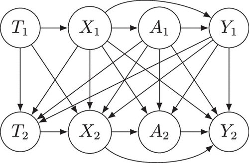
The DAG can be used to visualize the sets of parents. Although we cannot visualize the entire DAG for our variables, we can visualize the DAG restricted to a finite set. Figure 1 shows the DAG restricted to ${(T_k,X_k,A_k,Y_k)}_{k=1,2}$. It is worth noting that every DAG can be topologically ordered, which means that the nodes can be ordered in a way that ensures no node comes before its parents.

The second object is a Markov kernel from ${\mathcal{X}}^{(\text{Pa}(Z))}$ to ${\mathcal{X}}^{(Z)}$ for each Z. These Markov kernels tell us how to construct a variable Z in ${\cup }_{k\in \mathbb{N}}\{T_k,X_k,A_k,Y_k\}$ from its parents. They also tell how to construct new variables were we to modify the value of its parents. To ensure we can easily move between each set of variables, it is desirable to define the same probability measure for both. Thus, in addition to assuming the existence of Markov kernels, it benefits us to regard the original and new variables as arising from the same collection of independent variables, often referred to as exogenous variables. These considerations motivate defining Markov kernels as arising from a probability distribution for an exogenous variable and a deterministic assignment.

Assumption 2

(Causal Model: Markov Kernels). Assuming we have parents given by Assumption 1, each variable Z in the collection ${\cup }_{k\in \mathbb{N}}\{T_k,X_k,A_k,Y_k\}$ is associated with a Markov kernel ${\mathbb{P}}^{(Z)}$ from ${\mathcal{X}}^{(\text{Pa}(Z))}$ to ${\mathcal{X}}^{(Z)}$. We assume this Markov kernel can be expressed as

$${\mathbb{P}}^{(Z)}(B|\text{Pa}(Z))={\mathbb{P}}^{({\epsilon }_Z)}(\{w\in {\mathrm{\Omega }}^{(Z)}|f^{(Z)}(\text{Pa}(Z),w)\in B\}),$$

for some probability distribution ${\mathbb{P}}^{({\epsilon }_Z)}$ on $({\mathrm{\Omega }}^{(Z)},{\mathcal{E}}^{(Z)})$ and a measurable function $f^{(Z)}$ from ${\mathcal{X}}^{(\text{Pa}(Z))}\times {\mathrm{\Omega }}^{(Z)}$ to ${\mathcal{X}}^{(Z)}.$

To model ${(T_k,X_k,A_k,Y_k)}_{k\in \mathbb{N}}$ as an MPP, we require further conditions on the Markov kernels ensuring that, almost surely, the times are strictly increasing when finite and increasing otherwise, and the marks take the irrelevant mark exactly when the corresponding time is infinite. These assumptions are stated precisely in the Online Appendix (Assumption S.1). Our causal model, now comprised of sets of parents and Markov kernels, gives us a probability model for the variables we are interested in.

Assumption 3

(Causal Model: Distribution). Suppose that we have parents and kernels as given by Assumptions 1 and 2 and Assumption S.1 in the Online Appendix. We obtain the distribution $\mathbb{P}$ of a marked point process for ${(T_k,X_k,A_k,Y_k)}_{k\in \mathbb{N}}$ in two steps:

• Obtain a distribution $\mathbb{P}$ on the sequence of random variables ${({\epsilon }_{T_k},{\epsilon }_{X_k},{\epsilon }_{A_k},{\epsilon }_{Y_k})}_{k\in \mathbb{N}}$ with each ${\epsilon }_Z$ corresponding to the probability distribution ${\mathbb{P}}^{({\epsilon }_Z)}$ from Assumption 2 using the Ionescu Tulcea theorem with respect to their respective sequence of probability distributions.

• Assign iteratively $Z=f^{({\epsilon }_Z)}(\text{Pa}(Z),{\epsilon }_Z)$ for each variable Z in ${\cup }_{k\in \mathbb{N}}\{T_k,X_k,A_k,Y_k\}$

Finally, assume $K=\sup \{k:T_k<\infty \}$ under $\mathbb{P}$ is finite almost surely.

It is important to mention that the ordering in which variables are assigned reflects a topological ordering of our variables that is compatible with our DAG. Specifically, each variable Z must be defined after its parents are. In addition, we could have applied the Ionescu Tulcea theorem directly to the Markov kernels ${\mathbb{P}}^{(Z)}$ to arrive at the same distribution $\mathbb{P}$. However, as mentioned previously, it would be advantageous to fix the exogenous variables while manipulating the values of parents, so all our variables are defined with the same distribution $\mathbb{P}$.

3.5. Potential Outcomes

Markov kernels describe the conditional distribution of a variable as a function of its parents. Crucially, by replacing the parents in the Markov kernel with fixed values, we can examine what would have happened under different scenarios. Specifically, we focus on examining what would have occurred if we had fixed the values of $A_k$.

Definition 1

(Potential Outcomes). Suppose we have $\mathbb{P}$ on ${({\epsilon }_{T_k},{\epsilon }_{X_k},{\epsilon }_{A_k},{\epsilon }_{Y_k})}_{k\in \mathbb{N}}$ from Assumption 3. We start by fixing $B\subseteq \mathbb{N}$ and $a\in {\mathcal{X}}^{(A_{1:\infty })}$ representing the indices of jobs to be intervened and the values they take, respectively. We define potential outcomes

$${(T_k(a_B),X_k(a_B),A_k(a_B),Y_k(a_B))}_{k\in \mathbb{N}},$$

iteratively according to $Z(a_B)=f^{({\epsilon }_Z)}(\text{Pa}[a_B](Z),{\epsilon }_Z)$ for each Z in ${\cup }_{k\in \mathbb{N}}\{T_k,X_k,A_k,Y_k\}$, where we obtain $\text{Pa}[a_B](Z)$ by replacing each variable W in $\text{Pa}(Z)$ either with $a_k$ if W is $A_k$ and $k\in B$ or with $W(a_B)$ otherwise.

The sets $\text{Pa}[a_B](Z)$ give rise to a single world intervention graph (SWIG), where the nodes represent potential outcomes and the $a_k$, $k\in B$, and a directed edge exists from one variable to $Z(a_B)$ if the former is in the set $\text{Pa}[a_B](Z)$. To put it another way, if the variable $A_k$ for $k\in B$ was originally used to construct a subsequent variable, the potential outcome definition dictates we pass forward $a_k$ instead of $A_k(a_B)$. Even though $A_k(a_B)$ does not get passed forward, we still construct $A_k(a_B),$ which distinguishes the causal inference framework of Richardson and Robins (2013) from others.

Moreover, although other frameworks may make certain assumptions about potential outcomes, assumptions like consistency end up being a natural consequence (Malinsky et al. 2019).

Proposition 1

(Consistency). Let A any subset of ${\cup }_{k\in \mathbb{N}}\{A_k\}$. Suppose we have potential outcomes defined for $B\cup C\subseteq \mathbb{N}$ and $C\subseteq \mathbb{N}$ with $B\cap C=\varnothing$ and $a\in {\mathcal{X}}^{(A_{1:\infty })}$. For any Z in ${\cup }_{k\in \mathbb{N}}\{T_k,X_k,A_k,Y_k\}$ and among events for which $A_B(a_{B\cup C})=a_B$, the potential outcomes $Z(a_C)$ and $Z(a_{B\cup C})$ are equal.

To clarify, consistency implies that potential outcomes $Z(a_C)$ matches $Z(a_{B\cup C})$ when the potential outcome $A_B(a_{B\cup C})$ matches $a_B$. In essence, we need consistency so that $Y_k(a_B)$ has the same distribution as the original variable $Y_k$ when the intervention $A_B$ matches the value $a_B$ that we have fixed for the intervention. This enables us to substitute $Y_k(a_B)$ for $Y_k$ when we condition on $A_B=a_B$. The proof of consistency follows by noting that, under the conditions of the proposition, $Z(a_C)$ and $Z(a_{B\cup C})$ are expressed identically in terms of the exogenous variables ${\epsilon }^{(W)}$ and the assignment functions $f^{(W)}$ for W in ${\cup }_{k\in \mathbb{N}}\{T_k,X_k,A_k,Y_k\}$. This identity allows us to claim that potential outcomes are equal everywhere, as opposed to the weaker almost surely or in distribution.

The definition of potential outcomes leads us to another important concept called causal irrelevance, which tells us when we can drop the potential outcome notation. The SWIG induced by the potential outcome definition is the most convenient way to express causal irrelevance.

Proposition 2

(Causal Irrelevance). Suppose we have potential outcomes defined for $B\cup C\subseteq \mathbb{N}$ and $C\subseteq \mathbb{N}$ with $B\cap C=\varnothing$ and $a\in {\mathcal{X}}^{(A_{1:\infty })}$. If $Z(a_{B\cup C})$ is not a descendent of any $a_k$ with $k\in C$ in our SWIG, then the potential outcomes $Z(a_B)$ and $Z(a_{B\cup C})$ are equal.

In other words, if a potential outcome is not a descendant in the SWIG of an intervened value $a_k$, for $k\in B$, then the potential outcome is said to be causally irrelevant to the choice of $a_k$. In such cases, the value of the potential outcome does not change, whether we had passed $a_k$ forward at all. For example, since $T_1$ has no parents, then $T_1(a_B)$ is always equal to $T_1$. The proof of causal irrelevance is similar to that of consistency; that is, under the conditions of the proposition, $Z(a_B)$ and $Z(a_{B\cup C})$ are expressed identically in terms of the exogenous variables and the assignment functions.

After applying causal irrelevance, we visualize the SWIG restricted to ${(T_k(a_1),X_k(a_1),A_k(a_1),Y_k(a_1))}_{k=1,2}$ with $B=\{1\}$ in Figure 2. To obtain the SWIG from the original DAG, we split each node corresponding to $A_k$ for $k\in B$ into two nodes: one inheriting all incoming edges of $A_k$ and the other inheriting all outgoing edges.

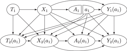
Causal irrelevance provides a useful way to reason about interference. In the causal inference literature, interference occurs when the potential outcomes of one individual are affected by the treatment assignment of other individuals (Hudgens and Halloran 2008). In our context, this means the potential outcomes for job k may depend on the decisions made for other jobs: In general, $X_k(a_B)\ne X_k$, $A_k(a_B)\ne A_k$, or $Y_k(a_B)\ne Y_k(a_k)$ for any set B that includes k and at least one other job. Figure 2 gives an example of interference, where the first job’s decision affects the second job’s potential outcomes. More broadly, the potential outcomes for job k are descendants in the SWIG of interventions on jobs $i\le k$, but not of those on jobs $i>k$. By causal irrelevance, decisions for earlier jobs may influence the potential outcomes of later jobs, but not the reverse.

A key advantage of SWIGs is that they uncover conditional independence relationships among potential outcomes. These relationships are a result of the SWIG being Markov compatible with the potential outcome distribution, which then implies local and global Markov properties. The local Markov property, for example, says that a variable is independent of its nondescendants when conditioning on its parents. The global Markov property characterizes conditional independence relationships arising from a property of the Markov compatible graph, known as d-separation. Although we will not delve into these concepts further in this paper, we will use two specific applications of the local Markov property of the SWIG.

Proposition 3

(Sequential Ignorability). Suppose we have potential outcomes defined for $B=\{k\}$ and $a\in {\mathcal{X}}^{(A_{1:\infty })}$. Let $R_{k+\mathcal{\ell }}$ be a vector of variables from $\text{Pa}(Y_{k+\mathcal{\ell }})\setminus A_k$ that includes $H_{k-1}$ and $X_k$, and let $R_{k+\mathcal{\ell }}(a_k)$ be the corresponding potential outcomes. Then, $Y_{k+\mathcal{\ell }}(a_k)$ is independent of $A_k$ conditional on $R_{k+\mathcal{\ell }}(a_k)$. As a result, we have

$$\mathbb{E}[Y_{k+\mathcal{\ell }}(a_k)|R_{k+\mathcal{\ell }}(a_k),T_{k+\mathcal{\ell }}(a_k)<\infty ]=\mathbb{E}[Y_{k+\mathcal{\ell }}(a_k)|R_{k+\mathcal{\ell }}(a_k),A_k,T_{k+\mathcal{\ell }}(a_k)<\infty ].$$

Proposition 4.

Suppose we have potential outcomes defined for $B=\{k\}$ and $a\in {\mathcal{X}}^{(A_{1:\infty })}$. Let $V_{k+\mathcal{\ell }}$ be a vector of variables from $\text{Pa}(Y_{k+\mathcal{\ell }})\setminus \{A_k,H_{k-1},X_k\}$, and let $V_{k+\mathcal{\ell }}(a_k)$ be the corresponding potential outcomes. Then, $V_{k+\mathcal{\ell }}(a_k)$ is independent of $A_k$ conditional on $H_{k-1}$ and $X_k$. As a result, we have

$$\mathbb{E}[A_k|H_{k-1},X_k,V_{k+\mathcal{\ell }}(a_k),T_{k+\mathcal{\ell }}(a_k)<\infty ]=\mathbb{E}[A_k|H_{k-1},X_k,T_{k+\mathcal{\ell }}(a_k)<\infty ].$$

A formal proof of these propositions is provided in Online Appendix S.2. To demonstrate these using the local Markov property, we first observe that the parents of $A_k$ are precisely $X_k$ and $H_{k-1}$. Additionally, because $a_k$ inherits all the outgoing edges of $A_k$ in the SWIG, $A_k$ has no descendants. This implies that every potential outcome, other than $A_k$, is a nondescendant of $A_k$ in the SWIG. We include $T_{k+\mathcal{\ell }}(a_k)<\infty$ in our conditioning event when taking expectations to avoid taking expectation of the irrelevant mark. These propositions state that $A_k$ provides no additional information about potential outcomes, and vice versa, even those occurring after the intervention on job k, beyond what is already known from the parents of $A_k$. This insight will be useful in the following sections, particularly when we include postintervention potential outcomes in our conditioning events. We refer the reader to Richardson and Robins (2013) and Malinsky et al. (2019) for more on Markov properties of SWIGs.

3.6. Lag Effect

Now that we have our causal model in place and our potential outcomes defined, we can focus on what we want to learn from the data. Our aim is to understand human sequential bias in the sense of how the potential outcome of a future job depends on whether the current job is subjected to a specific intervention. Let $\mathcal{\ell }>0$ denote the time lag between the current job being intervened upon and a future job that might be affected by it. We refer to job $k+\mathcal{\ell }$ as the future job and job k as the current job. We can consider the potential outcomes as defined in Definition 1 with $B=\{k\}$ and $a_k\in \{0,1\}$ to capture this idea. According to causal irrelevance (Proposition 2), we have $T_i(a_k)=T_i$, $X_i(a_k)=X_i$, and $A_i(a_k)=A_i$ when $i\le k$; $Y_i(a_k)=Y_i$ when $i<k$. Otherwise, we cannot drop the potential outcome notation. Provided it is not the irrelevant mark, we are interested in $Y_{k+\mathcal{\ell }}(a_k)$, which represents the outcome for the future job we would have observed if the current job was forced to take intervention $a_k$. Although we cannot learn about individual potential outcomes $Y_{k+\mathcal{\ell }}(a_k)$, we can estimate their expectations in various situations:

Definition 2

(Lag Effects). Suppose we have potential outcomes given by Definition 1 for $B=\{k\}$ and $a_k=1$ and separately for $a_k=0$. Let $R_{k+\mathcal{\ell }}$ be a vector of variables from $\text{Pa}(Y_{k+\mathcal{\ell }})\setminus A_k$ that includes $H_{k-1}$ and $X_k$, and let $R_{k+\mathcal{\ell }}(a_k)$ be the corresponding potential outcomes. Introduce for $k,\mathcal{\ell }\in \mathbb{N}$,

$$\zeta (k,\mathcal{\ell },r)=\mathbb{E}\left[Y_{k+\mathcal{\ell }}(1)|R_{k+\mathcal{\ell }}(1)=r,T_{k+\mathcal{\ell }}(1)<\infty \right]-\mathbb{E}\left[Y_{k+\mathcal{\ell }}(0)|R_{k+\mathcal{\ell }}(0)=r,T_{k+\mathcal{\ell }}(0)<\infty \right].$$

This represents the average causal effect on job $k+\mathcal{\ell }$ after intervening on job k among specific events for which $T_{k+\mathcal{\ell }}(a_k)<\infty$ and $R_{k+\mathcal{\ell }}(a_k)=r$ under the respective intervention.

In the definition above, the expectation is taken with respect to the probability distribution $\mathbb{P}$, holding the interventions for the first $k-1$ jobs fixed and only varying the intervention for job k. The lag effect reflects how the outcome for a future job ($k+\mathcal{\ell }$) changes as a result of the intervention at job k, for given indices k and $k+\mathcal{\ell }$. To ensure the effect is well defined, we restrict attention to cases where the future job $k+\mathcal{\ell }$ actually occurs under the intervention (i.e., $T_{k+\mathcal{\ell }}(a_k)<\infty$), thereby avoiding situations involving irrelevant marks.

In the above definition, we compute expectation with respect to the probability distribution $\mathbb{P}$ while holding the interventions of the first $k-1$ jobs at their original values and varying only the intervention for job k. The lag effect may depend on the index k of the current job and the index of $k+\mathcal{\ell }$ of the future job. To avoid computing the irrelevant mark, we condition on $T_{k+\mathcal{\ell }}(a_k)<\infty$.

With the lag effect, we are essentially comparing what happens to future potential outcomes when we make one decision versus another for an earlier job. For example, if we choose $a_k=1$ for job k, we check how this affects the outcome of a later job, averaging over all cases where a certain condition would have been met. We then compare this to what would happen if we made a different decision for job k, $a_k=0$, and again observe the average outcome for the later job under similar conditions. This lets us measure how an earlier decision influences later outcomes, helping to reveal sequential human bias. If there is no influence, the decision for one job would not affect future outcomes, and the lag effect will be zero. But if influence is present, the lag effect may be positive or negative, showing whether intervening ($a_k=1$ versus $a_k=0$) leads to better or worse average outcomes for future jobs.

To make this more concrete, suppose we want to estimate how a routing decision for patient k (for example, assigning them to usual care versus a new care pathway) affects the number of tests ordered for the next patient, $k+1$, focusing specifically on scenarios where patient $k+1$ has blood pressure in the normal range at the time they receive care. To do this, we first imagine all situations where patient k receives usual care; we look at the subset of these where, as a consequence, patient $k+1$ is present and has normal blood pressure, and we calculate the average number of tests ordered. Next, we repeat this process for the scenario where patient k receives the new care pathway: We again focus only on cases where, as a result of that decision, patient $k+1$ is present and has normal blood pressure, and compute the average outcome. The lag effect is the difference between these two averages. Importantly, the groups being compared may consist of different patients because the decision for patient k can influence both whether patient $k+1$ presents for care and what their blood pressure is at the time of care.

It is important to understand the causal query being asked with the lag effect, because it is subtle. We expose job k to intervention $a_k=1$ and average the resulting value of $Y_{k+\mathcal{\ell }}$ over all events which consequently attain a certain level for $R_{k+\mathcal{\ell }}$ (possibly postintervention) and yield observations at time period $k+\mathcal{\ell }$. This scenario is then contrasted to exposing job k to intervention $a_k=0$ instead and averaging the resulting value of $Y_{k+\mathcal{\ell }}$ over all events which consequently attain the same level for $R_{k+\mathcal{\ell }}$ and yield observations at time period $k+\mathcal{\ell }$. Our causal query is also distinctly different than what it would be were we to use:

This asks what would happen under different interventions among events who actually attain a certain level of $R_{k+\mathcal{\ell }}$ and yield observations at time period $k+\mathcal{\ell }$ under the realized intervention. Although neither are conventional, Pearl has a nice discussion on distinguishing between these two causal queries (Pearl 2015) and why someone might condition on postintervention variables.

For us, we have chosen this lag effect based on practical considerations. One important consideration is that we need to condition on at least one postintervention event, specifically the event where the induced $Y_{k+\mathcal{\ell }}$ is observed. This is necessary to avoid computing expectations of irrelevant marks and is unavoidable when the number of jobs, K, is random and influenced by interventions. This situation is common in many stochastic service systems, such as those that process jobs at different rates depending on prior interventions and in a fixed time frame (e.g., 9 a.m. to 5 p.m.).

Returning to our example, suppose instead we focused on the latter causal inquiry: estimating the effect of patient k’s routing decision on the next patient’s outcome, but only among those who actually show up for care with normal blood pressure under the observed pathway. The problem here is that, under a different decision for patient k, some of these patients might not even appear for care, making their outcome undefined in the alternative scenario. Even if they do appear, their blood pressure could be different as a consequence of the earlier decision (perhaps they had to wait longer), so observed differences might simply reflect changes in clinical context rather than a difference in how decisions are made.

Another factor to consider is that, although the latter causal query, which conditions on realized values, may be more straightforward to comprehend, it is generally not identifiable. The latter query is equivalent to conditioning on colliders (e.g., $T_{k+\mathcal{\ell }}$) between the intervention $A_k$ and the potential outcome $Y_{k+\mathcal{\ell }}(a_k)$, thereby opening up a path to transmit noncausal associations from $A_k$ to $Y_{k+\mathcal{\ell }}(a_k)$. The only way to close the path is to condition on potential outcomes related to postintervention variables (such as $T_{k+\mathcal{\ell }}(a_k)$). The two causal queries would coincide if the conditioning event $\{R_{k+\mathcal{\ell }}(a_k)=r,T_{k+\mathcal{\ell }}(a_k)<\infty \}$ remains invariant to $a_k$. For example, if $R_{k+\mathcal{\ell }}$ only includes preintervention variables such as $H_{k-1}$ and $X_k$, and the intervention has no impact on whether the subsequent $Y_{k+\mathcal{\ell }}$ is observed, then $\{R_{k+\mathcal{\ell }}(a_k)=r,T_{k+\mathcal{\ell }}(a_k)<\infty \}$ could be invariant to $a_k$. Yet, as noted above, we anticipate that the latter condition may be too restrictive for many stochastic systems.

A final consideration was what variables should we allow in the conditioning set. We choose to require $H_{k-1}$ and $X_k$ in $R_{k+\mathcal{\ell }}$ for reasons that we will discuss in the next section, because they are relevant to identifying the causal effect. We allow for variables that occur postintervention, but prior to $Y_{k+\mathcal{\ell }}$, so we later can better model the variation in $Y_{k+\mathcal{\ell }}$. For example, the future job’s characteristics $X_{k+\mathcal{\ell }}$ may have a larger influence on the outcome $Y_{k+\mathcal{\ell }}$ than the current job’s characteristics $X_k$. More generally, we can include any variable from $\text{Pa}(Y_{k+\mathcal{\ell }})\setminus A_k$ in $R_{k+\mathcal{\ell }}$. In addition to $X_k$ and $H_{k-1}$, these variables include the characteristics, interventions, and outcomes of any job between k and $\mathcal{\ell }$ (i.e., $A_j$, $X_j$, $Y_j$ for $j=k+1$ to $j=\mathcal{\ell }-1$), the outcome of job k ($Y_k$), and the characteristics and intervention of job $k+\mathcal{\ell }$ ($X_{k+\mathcal{\ell }}$ and $A_{k+\mathcal{\ell }}$). We also consider these postintervention variables to focus on the direct effects of the intervention, which fix the induced value of these variables to a certain level. For instance, we may wish to determine if directing a patient to vertical flow in the ED would speed up service for a future job, even were the induced congestion levels held constant.

At this point, it is useful to clarify why our lag effect is closely related to, but more general than, the DTR causal effects studied by Boruvka et al. (2018). When the number of jobs K is fixed and finite, the structural causal model for ${(X_k,A_k,Y_k)}_{k\in \mathbb{N}}$ coincides with that of a DTR, with $X_k$, $A_k$, and $Y_k$ playing the roles of time-varying covariates, treatment assignments, and outcomes at decision epoch k. In this case, the conditioning event $\{T_{k+\mathcal{\ell }}(a)<\infty \}$ is deterministic and can be dropped from the lag effect. If we further restrict $R_{k+\mathcal{\ell }}$ to variables observed prior to the current decision (i.e., $H_{k-1}$ and $X_k$), the lag effect $\zeta (k,\mathcal{\ell },r)$ reduces exactly to the causal effects in Boruvka et al. (2018). Consequently, many of the arguments developed for DTRs can be reused here, with additional care only needed to accommodate random K and conditioning on postintervention variables.

We may find it too difficult to specify the right functional form to express the influence of r on the lag effect $\zeta (k,\mathcal{\ell },r)$, because r can be a large vector. The vector r represents possible values of $R_{k+\mathcal{\ell }}(a_k)$, which itself is a vector of real-valued random variables that includes the prior history $H_{k-1}$ and current characteristics $X_k$. The size of r grows linearly in size as k increases. For instance, if $X_k$ captures one characteristic (e.g., age) and $R_{k+\mathcal{\ell }}(a_k)$ includes only $H_{k-1}$ and $X_k$, then r would be $(3k-2)$-dimensional. This accounts for three real-valued random variables from each prior job and one real-valued random variable from the current job. In these cases, it may be beneficial to use marginalization to reduce the dimension of the lag effect and then express the functional form for this lower-dimensional effect. One way to accomplish this is with the following.

Definition 3

(Marginalized Lag Effects). Consider the lag effect $\zeta (k,\mathcal{\ell },r)$ as it is given in Definition 2. Let $S_{k+\mathcal{\ell }}$ be any (possibly empty) subset of $R_{k+\mathcal{\ell }}$. Introduce

$${\zeta }_{\text{marg}}(k,\mathcal{\ell },s)=\mathbb{E}\left[\zeta (k,\mathcal{\ell },R_{k+\mathcal{\ell }})|S_{k+\mathcal{\ell }}=s,T_{k+\mathcal{\ell }}<\infty \right].$$

This represents the lag effect marginalized over $R_{k+\mathcal{\ell }}$ conditional on $S_{k+\mathcal{\ell }}$ and $T_{k+\mathcal{\ell }}<\infty$.

If $S_{k+\mathcal{\ell }}=R_{k+\mathcal{\ell }}$, then the lag effect and the marginalized lag effect are equivalent. Our choice of the marginalized lag effect is also guided by practical considerations. In this case, our concern is not about identification. Identifying the marginalized lag effect can be achieved once the lag effect is identified. However, it is possible to condition on potential outcomes instead of observed variables. This would result in an identifiable effect, which can be calculated through a parametric g-formula (Robins 1986). However, this approach requires a full specification of the Markov kernels, which we find too restrictive. As we saw before, if the conditioning event $\{R_{k+\mathcal{\ell }}(a_k)=r,T_{k+\mathcal{\ell }}(a_k)<\infty \}$ remains invariant to $a_k$, then the two strategies coincide, and the marginalized lag effect is simply:

3.7. Identification

The primary challenge in causal inference is that we can only observe one of the potential outcomes, namely either $Y_{k+\mathcal{\ell }}(1)$ or $Y_{k+\mathcal{\ell }}(0)$. As a result, we are generally unable to estimate the lag effect (as defined in Definition 2). We need to extrapolate from our observations of $Y_{k+\mathcal{\ell }}(1)$ when the intervention is assigned to $A_k=1$ in order to make inferences about $Y_{k+\mathcal{\ell }}(1)$ when the intervention is assigned to $A_k=0$. For such extrapolation to be valid, we require the assumption of positivity in addition to consistency, causal irrelevance, and sequential ignorability (as outlined in Propositions 1–3). This assumption states that every job has a chance of being assigned to the intervention.

Assumption 4

(Positivity). Consider $R_{k+\mathcal{\ell }}$ as defined for the lag effect (Definition 2). Assume

$$\mathbb{E}[A_k|R_{k+\mathcal{\ell }},T_{k+\mathcal{\ell }}<\infty ]\in (0,1)$$

almost surely.

With positivity and the other properties, we are able to identify the lag effect, which is to say that we can re-express the lag effect equivalently in terms of observed variables.

Lemma 1

(Nonparametric Identification). Consider the lag effect $\zeta (k,\mathcal{\ell },r)$ as it is given in Definition 2. Assuming positivity (Assumption 4), then the lag effect $\zeta (k,\mathcal{\ell },r)$ is equivalent to

$$\mathbb{E}[Y_{k+\mathcal{\ell }}|A_k=1,R_{k+\mathcal{\ell }}=r,T_{k+\mathcal{\ell }}<\infty ]-\mathbb{E}[Y_{k+\mathcal{\ell }}|A_k=0,R_{k+\mathcal{\ell }}=r,T_{k+\mathcal{\ell }}<\infty ].$$

Proof.

Sequential ignorability (Proposition 3) implies that, conditional on $R_{k+\mathcal{\ell }}(a_k)$, the treatment assignment $A_k$ is independent of the potential outcome $Y_{k+\mathcal{\ell }}(a_k)$. This allows us to write the following:

$$\mathbb{E}[Y_{k+\mathcal{\ell }}(a_k)|R_{k+\mathcal{\ell }}(a_k)=r,T_{k+\mathcal{\ell }}(a_k)<\infty ]=\mathbb{E}[Y_{k+\mathcal{\ell }}(a_k)|A_k=a_k,R_{k+\mathcal{\ell }}(a_k)=r,T_{k+\mathcal{\ell }}(a_k)<\infty ].$$

Observe that the conditioning event includes $A_k=a_k$, so the conditional expectation is taken only over samples where $A_k=a_k$. By causal irrelevance (Proposition 2), we have $A_k(a_k)=A_k$, because $A_k(a_k)$ is not a descendant of $a_k$ in the SWIG. Therefore, we are equivalently conditioning on the event $A_k(a_k)=a_k$. This is exactly the setting where we can invoke consistency (Proposition 1) for sets $B=\{k\}$ and $C=\varnothing$. Consistency then guarantees that for any potential outcome $Z(a_k)$ equals Z whenever $A_k(a_k)=a_k$. In other words, if $A_k(a_k)=a_k$, then $R_{k+\mathcal{\ell }}(a_k)=R_{k+\mathcal{\ell }}$, $T_{k+\mathcal{\ell }}(a_k)=T_{k+\mathcal{\ell }}$ and $Y_{k+\mathcal{\ell }}(a_k)=Y_{k+\mathcal{\ell }}$. This justifies replacing the potential outcomes in the conditional expectation with their observed counterparts:

$$\mathbb{E}[Y_{k+\mathcal{\ell }}(a_k)|A_k=a_k,R_{k+\mathcal{\ell }}(a_k)=r,T_{k+\mathcal{\ell }}(a_k)<\infty ]=\mathbb{E}[Y_{k+\mathcal{\ell }}|A_k=a_k,R_{k+\mathcal{\ell }}=r,T_{k+\mathcal{\ell }}<\infty ].$$

Positivity (4) then ensures this quantity is defined for both $a_k=1$ and $a_k=0$. Applying these expressions to $a_k=1$ and $a_k=0$, we arrive at

$$\begin{array}{ll}\zeta (k,\mathcal{\ell },r)\hfill & =\mathbb{E}[Y_{k+\mathcal{\ell }}(1)\hspace{0.17em}|\hspace{0.17em}{R}_{k+\mathcal{\ell }}(1)=r,T_{k+\mathcal{\ell }}(1)<\infty ]-\mathbb{E}[Y_{k+\mathcal{\ell }}(0)\hspace{0.17em}|\hspace{0.17em}{R}_{k+\mathcal{\ell }}(0)=r,T_{k+\mathcal{\ell }}(0)<\infty ]\hfill \\ \hfill & =\mathbb{E}[Y_{k+\mathcal{\ell }}\hspace{0.17em}|\hspace{0.17em}{A}_k=1,R_{k+\mathcal{\ell }}=r,T_{k+\mathcal{\ell }}<\infty ]-\mathbb{E}[Y_{k+\mathcal{\ell }}\hspace{0.17em}|\hspace{0.17em}{A}_k=0,R_{k+\mathcal{\ell }}=r,T_{k+\mathcal{\ell }}<\infty ],\hfill \end{array}$$

completing the proof. □

4. Estimation

4.1. Estimating Equation

Our goal is to estimate marginalized lag effects ${\zeta }_{\text{marg}}(k,\mathcal{\ell },s)$ using estimating equations for a fixed $\mathcal{\ell }\in \mathbb{N}$. Suppose we have collected data on n panels. These data are assumed to be comprised of n independent and identically distributed (i.i.d.) realizations of our marked point process ${(T_k,X_k,A_k,Y_k)}_{k\in \mathbb{N}}$ modeled with distribution $\mathbb{P}$. We do not assume $T_k$ is observed or use irrelevant marks for estimation, so that observations are restricted to the vector ${(X_k,A_k,Y_k)}_{k\in \{1,\dots ,K\}}$. Let $\mathbb{E}$ denote expectation with respect to $\mathbb{P}$ and ${\mathbb{E}}_n$ denote the empirical average with respect to n i.i.d. realizations of our marked point process.

The primary estimating function we work with is of the form

wherefor parameters $\alpha ,\beta ,\xi ,\eta$ that we wish to estimate and suitable functions g and f that depend on $\xi$ and $\eta$. We search for parameters $\theta ≔(\xi ,\eta ,\alpha ,\beta )$ that solve Equation (1) in some compact subset $\mathrm{\Theta }$ of ${\mathbb{R}}^m$. To simplify notation, we dropped the dependence of functions on parameters. The variable $U_k$ can be decomposed into several parts:

• $W_k$ (a weight for mitigating bias and emphasizing certain data points)

• $Y_{k+l}$ (outcome of future job)

• $g{(R_{k+\mathcal{\ell }})}^{\prime }\alpha$ (a linear working model for the baseline conditional mean of $Y_{k+\mathcal{\ell }}$)

• $f{(S_{k+\mathcal{\ell }})}^{\prime }\beta$ (a linear working model for the marginalized lag effect)

• $\left[\begin{array}{c}g(R_{k+\mathcal{\ell }})\\ A_{k}f(S_{k+\mathcal{\ell }})\end{array}\right]$ (derivative of the working mean model $g{(R_{k+\mathcal{\ell }})}^{\prime }\alpha +A_{k}f{(S_{k+\mathcal{\ell }})}^{\prime }\beta$ with respect to $\alpha$, $\beta$)

In particular, the parameter $\beta$ is the inferential target, because it contributes to the marginalized linear working model for the lag effect. If K were deterministic, then the estimating equation (Equation (1)) has several precedents. It is akin to a generalized estimating equation (GEE), in which data are weighted, clustered into panels, and given an independent working correlation matrix. It is also akin to the g-estimation approach of Vansteelandt and Sjolander (2016) for structural nested mean models and the weighted and centered approach of Boruvka et al. (2018).

Although not the inferential target, the estimating equation depends on parameters $\xi$ and $\eta$. These parameters specify a working model for conditional probabilities of job k’s intervention assignment:

We assume $\xi$ is also estimated using an estimating equation of the form

for variables $L_k{\mathrm{𝟙}}_{\{k\le K\}}$ that depends only on $\xi$ and the observations of ${(X_k,A_k,Y_k)}_{k\in \{1,\dots ,K\}}$. Similarly, we assume $\eta$ is also estimated using an estimating equation of the formfor variables $M_k{\mathrm{𝟙}}_{\{k\le K\}}$ that depends only on $\eta$ and the observations of ${(X_k,A_k,Y_k)}_{k\in \{1,\dots ,K\}}$. Most likely, $\xi$ and $\eta$ would be estimated using logistic or log-linear regression. For example, if we used logistic regression and assumed a linear model in $S_{k+\mathcal{\ell }}$ on the log-odds scale with $\xi$ as the regression coefficients, our estimating equation might use:

By stacking the estimating equations together,

and estimation can be viewed as searching for $\alpha$, $\beta$, $\xi$, and $\eta$ that solve the stacked estimating equation. If we define $U_{\text{stacked}}$ as the concatenated vector of U, L, and M, then for Equation (2) to be meaningful, we are assuming that $U_{\text{stacked}}$ is integrable. Because these variables are sums of a random number of variables, we impose mild conditions on K and $U_k$, $L_k$, and $M_k$ to recover integrability (see Assumption S.2 in the Online Appendix) to recover integrability.

Lemma 2

(Integrability). Under the conditions on $U_k$, $L_k$, $M_k$, and K in Assumption S.2, Equation (2) is well defined in the sense that, for each $\theta \in \mathrm{\Theta }$, $U_{\text{stacked}}$ is integrable and has finite expectation.

The assumptions can be found in the Online Appendix S.1 and the proof in Online Appendix S.3. The broad arc is to replace the random sum in the definition of $U_{\text{stacked}}$ with an infinite sum and then exchange the expectation and the infinite sum. The conditions in Assumption S.2 are then used to ensure that the final sum can be bounded above by the expectation of K up to a constant.

4.2. Estimating Procedure

The first step of estimation would be to use the observations of ${(X_k,A_k,Y_k)}_{k\in \{1,\dots ,K\}}$ to recover an estimate ${\xi }_n$ and ${\eta }_n$ that solves the estimating equations ${\mathbb{E}}_n[U]={\mathbb{E}}_n[V]=0$. For example, we might use logistic regression to model the above conditional probabilities on the log odds scale as a linear function of the $S_{k+\mathcal{\ell }}$ or $R_{k+\mathcal{\ell }}$. In such a case, the parameters ${\xi }_n$ and ${\eta }_n$ would be the estimated regression coefficients. In special circumstances, the intervention $A_k$ was randomized according to a known probability. Consequently, $q_k(S_{k+\mathcal{\ell }};\xi )$ and $p_k(R_{k+\mathcal{\ell }};\eta )$ would be exact.

Once $\xi$ and $\eta$ are estimated, we turn to specifying $W_k$, f, and g. The weight term $W_k$ is taken to be the ratio of the two conditional probability models:

Naturally, we are assuming that we are not dividing by zero; otherwise, the weights would be ill defined. This assumption is the empirical equivalent of our positivity (assumption Assumption 4). These weights resemble (stabilized) inverse probability weights, in which a job is weighted inversely according to the probability of receiving their realized intervention assignment (Horvitz and Thompson 1952). Jobs that are more likely to receive their realized intervention assignment are subsequently down-weighted relative to those that are less likely. Given that certain jobs may be predisposed to be assigned a particular intervention, the weights create a pseudo-population of jobs in each intervention group that better reflects all jobs and not just those in the given intervention group. In the special case when $S_{k+\mathcal{\ell }}=R_{k+\mathcal{\ell }}$ or when $p_k(R_{k+\mathcal{\ell }};{\eta }_n)=q_k(S_{k+\mathcal{\ell }};{\xi }_n)$, then the weights $W_k$ are just one.

Meanwhile, we specify $f(S_{k+\mathcal{\ell }})$ to be any vector-valued function of $S_{k+\mathcal{\ell }}$. It reflects our assumptions about how we think the marginalized lag effect might vary as a function of $S_{k+\mathcal{\ell }}$, that is,

For example, we might think the marginalized lag effect of assigning a patient to vertical flow is quadratic in a patient’s age. If $S_{k+\mathcal{\ell }}$ were the current patient’s age, then we might chose

We can similarly specify the baseline term $g(R_{k+\mathcal{\ell }})$ to be any vector-valued function of $R_{k+\mathcal{\ell }}$ with one caveat. It must contain the variable $q_k(S_{k+\mathcal{\ell }};\xi )f(S_{k+\mathcal{\ell }})$. This caveat is so that the working mean model:

upon a redefinition of $\alpha$, includes the model in which the $A_k$ is centered:

Including $q_k(S_{k+\mathcal{\ell }};\xi )f(S_{k+\mathcal{\ell }})$ in $g(R_{k+\mathcal{\ell }})$ follows the strategy of Vansteelandt and Sjolander (2016) of making the mean model more general while still, practically, centering the intervention assignments. Centering is recommended for reasons we discuss later and is recommended in Boruvka et al. (2018).

The last step of estimation is to search for a solution ${\alpha }_n$ and ${\beta }_n$ to the estimating equation (Equation (1)). Given the similarity of Equation (1) to GEE, these parameters (although not necessarily their standard errors) can be estimated using standard GEE software, provided the working correlation matrix is specified to be independent. We next study the properties of the resulting estimator ${\beta }_n$.

4.3. Consistency and Asymptotic Normality

Our estimator is a type of estimator called a Z-estimator (Z for “zero”), as it involves searching for roots of an estimating equation. Asymptotic properties of Z-estimators have been extensively studied, so that we can invoke standard arguments. In an effort to be self-contained, we sketch the arguments in Van der Vaart (2000). We start with the following definition.

Definition 4

(Estimator). Define an estimator ${\theta }_n=({\xi }_n,{\eta }_n,{\alpha }_n,{\beta }_n)$ to be a solution in a set $\mathrm{\Theta }\subseteq {\mathbb{R}}^m$ to the (stacked) estimating equation (Equation (2)), should such a solution exist. Define ${\theta }_{\infty }=({\xi }_{\infty },{\eta }_{\infty },{\alpha }_{\infty },{\beta }_{\infty })$ to be a solution in $\mathrm{\Theta }$ to the asymptotic version of the estimating equation:

$$\mathbb{E}\left[U_{\text{stacked}}\right]=0,$$

should such a solution exist.

The first property of our estimators is consistency.

Theorem 1

(Consistency). Under Assumption S.3, the estimator ${\theta }_n$ in Definition 4 is consistent with respect to ${\theta }_{\infty }$:

$${\theta }_n\stackrel{P}{\to }{\theta }_{\infty }.$$

Proof.

The proof follows from theorem 5.7 in Van der Vaart (2000) if two conditions are met. Take $M_n(\theta )=-\Vert \begin{array}{c}{\mathbb{E}}_n[U_{\text{stacked}}]\end{array}\Vert$ and $M(\theta )=-\Vert \begin{array}{c}\mathbb{E}[U_{\text{stacked}}]\end{array}\Vert$. The first condition is the uniform convergence of $M_n(\theta )$ to $M(\theta )$ in probability over $\mathrm{\Theta }$. Given that ${\mathbb{E}}_n[U_{\text{stacked}}]$ is the empirical average over i.i.d. samples of $U_{\text{stacked}}$, this uniform convergence is an application of a uniform law of large numbers and follows from several conditions, including compactness of $\mathrm{\Theta }$ in ${\mathbb{R}}^m$, finiteness of $\mathbb{E}[U_{\text{stacked}}]$ (Lemma 2), and the mapping $\theta \to U_{\text{stacked}}$ being almost surely continuous and dominated by an appropriate function (see lemma 1 in Tauchen (1985)). The second condition, known as well separatedness, is a property of the maximizer of a function. Specifically, the maximizer ${\theta }_{\infty }$ of $M(\theta )$ is well separated if it satisfies

$$\underset{\theta \in \mathrm{\Theta }:\Vert \begin{array}{c}\theta -{\theta }_{\infty }\end{array}\Vert \ge ϵ}{\sup }M(\theta )<M({\theta }_{\infty })$$

for any $ϵ>0$. This condition ensures that only parameters very close to ${\theta }_{\infty }$ can yield values of $M(\theta )$ that are near the maximum $M({\theta }_{\infty })$. Well separatedness follows immediately from the uniqueness of the maximizer and the almost sure continuity of the mapping $\theta \to U_{\text{stacked}}$ over compact $\mathrm{\Theta }$ (Assumption S.3). The proof of theorem 5.7 in Van der Vaart (2000) uses the uniform convergence condition to argue that $M({\theta }_n)\stackrel{P}{\to }M({\theta }_{\infty })=0$. Well separatedness then ensures that the only way $M({\theta }_n)$ converges in probability to zero would be if ${\theta }_n$ were converging in probability to $\theta$. $\square$

The assumptions required for consistency (Assumption S.3) in common choices of L and M (such as logistic or log-linear models) are relatively mild. Continuity of $\theta \to U_{\text{stacked}}$ is reasonable, because U is linear in $\alpha$ and $\beta$ and smooth in $\xi$, and L and M are constant in $\alpha$ and $\beta$ and smooth in $\xi$ and $\eta$. The main concern is that U involves division by $p_k(R_{k+\mathcal{\ell }};\eta )$ or $1-p_k(R_{k+\mathcal{\ell }};\eta )$, which could prevent continuity over $\mathrm{\Theta }$ if $p_k(R_{k+\mathcal{\ell }};\eta )$ is not bounded away from zero and one. For a function to dominate the mapping $\theta \to U_{\text{stacked}}$, K and variables contributing to $U_k$ cannot be too large. This is comparable to the conditions for integrability (Assumption S.2). In practice, these variables are usually bounded. Similarly, parameters are usually bounded in practice, so compactness of $\mathrm{\Theta }$ is usually not an issue.

The second property of our estimators is $\sqrt{n}$-consistency and asymptotic normality.

Theorem 2

(Asymptotic Normality). Under Assumption S.4, the estimator ${\theta }_n$ in Definition 4 is $\sqrt{n}$-consistent with respect to ${\theta }_{\infty }$:

$$\sqrt{n}({\theta }_n-{\theta }_{\infty })=-{\mathbb{B}}^{-1}\sqrt{n}{E}_n\left[U_{\text{stacked}}{|}_{\theta ={\theta }_{\infty }}\right]+o_p(1)$$

and asymptotically normal with mean ${\theta }_{\infty }$ and variance ${\mathbb{B}}^{-1}\mathbb{C}{({\mathbb{B}}^{-1})}^{\prime }$, where

$$\mathbb{B}=\mathbb{E}\left[{\nabla }_{\theta }{U}_{\text{stacked}}{|}_{\theta ={\theta }_{\infty }}\right];\hspace{1em}\hspace{1em}\mathbb{C}=\mathbb{E}\left[U_{\text{stacked}}{U}_{\text{stacked}}^{\prime }{|}_{\theta ={\theta }_{\infty }}\right].$$

Proof.

The proof follows from several results in Van der Vaart (2000), including theorem 5.21, lemma 19.24, and example 19.7. Let $\mathrm{\Psi }(\theta )=\mathbb{E}[U_{\text{stacked}}]$ and ${\mathrm{\Psi }}_n(\theta )={\mathbb{E}}_n[U_{\text{stacked}}]$, such that $\mathrm{\Psi }({\theta }_{\infty })={\mathrm{\Psi }}_n({\theta }_n)=0$. We can obtain an approximation for $\sqrt{n}\mathrm{\Psi }({\theta }_n)$ from $\mathrm{\Psi }({\theta }_{\infty })=0$ and the differentiability of $\mathrm{\Psi }(\theta )$ at ${\theta }_{\infty }$:

$$\sqrt{n}\mathrm{\Psi }({\theta }_n)=\sqrt{n}\hspace{0.17em}\mathbb{B}·({\theta }_n-{\theta }_{\infty })+\sqrt{n}\Vert \begin{array}{c}{\theta }_n-{\theta }_{\infty }\end{array}\Vert o_P\left(1\right).$$

Meanwhile, the central limit theorem allows us to conclude that $\sqrt{n}{\mathrm{\Psi }}_n({\theta }_{\infty })$ is asymptotically normal with mean zero and covariance $\mathbb{C}.$ The challenge is to connect the two aforementioned results through empirical process theory, which necessitates demonstrating that $\sqrt{n}{\mathrm{\Psi }}_n({\theta }_{\infty })+\sqrt{n}\mathrm{\Psi }({\theta }_n)\stackrel{P}{\to }0$. This connection relies on the compactness of $\mathrm{\Theta }$ and the (almost sure) Lipschitz continuity of $\theta \to U_{\text{stacked}}$, which provides uniform convergence in distribution over $\mathrm{\Theta }$ of the empirical process $\sqrt{n}({\mathrm{\Psi }}_n(\theta )-\mathrm{\Psi }(\theta ))$. Thus, we can deduce the following:

$$\sqrt{n}\hspace{0.17em}\mathrm{\Psi }({\theta }_n)=\sqrt{n}\hspace{0.17em}\mathbb{B}·({\theta }_n-{\theta }_{\infty })+\sqrt{n}\hspace{0.17em}\Vert \begin{array}{c}{\theta }_n-{\theta }_{\infty }\end{array}\Vert \hspace{0.17em}{o}_P\left(1\right)=-\sqrt{n}\hspace{0.17em}{\mathrm{\Psi }}_n({\theta }_{\infty })+o_P(1).$$

Last, we argue $\sqrt{n}\hspace{0.17em}\Vert \begin{array}{c}{\theta }_n-{\theta }_{\infty }\end{array}\Vert \hspace{0.17em}{o}_P(1)=o_P(1)$ because $\sqrt{n}{\mathrm{\Psi }}_n({\theta }_{\infty })=O_P(1)$ and because $\mathbb{B}$ is invertible as specified in Assumption S.4. □

The additional assumptions required for asymptotic normality (Assumption S.4) in common choices of L and M (such as logistic or log-linear models) are relatively mild. Similar to continuity, it is reasonable to assume Lipschitz continuity and differentiability for the mapping $\theta \to U_{\text{stacked}}$, because $U_{\text{stacked}}$ is a smooth function over $\mathrm{\Theta }$ with $p_k(R_{k+\mathcal{\ell }};\eta )$ bounded away from zero and one if needed. Finiteness of $\mathbb{B}$ is linked to integrability and finding a dominating function for $\theta \to U_{\text{stacked}}$ and requires that K and the variables contributing to $U_k$ cannot be too large. Invertibility of $\mathbb{B}$ follows from the uniqueness of our minimizer ${\theta }_{\infty }$. The main concern is the finiteness of $\mathbb{C}$ and the square-integrability of the Lipschitz constant, which further limits the size of K and the variables contributing to $U_k$.

4.4. Double Robustness

Our next task is to connect ${\beta }_{\infty }$, for which ${\beta }_n$ is consistent, to the marginalized lag effect ${\xi }_{\text{marg}}(k,\mathcal{\ell },s)$. We can make this connection if some of our various modeling assumptions is correct. All told, there are four different models that we wish were valid for some $\theta \in \mathrm{\Theta }$:

• Outcome model, viz,

  $$g{(R_{k+\mathcal{\ell }})}^{\prime }\alpha +A_{k}f{(S_{k+\mathcal{\ell }})}^{\prime }\beta =\mathbb{E}[Y_{k+\mathcal{\ell }}|R_{k+\mathcal{\ell }},A_k,T_{k+\mathcal{\ell }}<\infty ].$$(4)

• Conditional probability model in the numerator of the weights, viz,

  $$q_k(S_{k+\mathcal{\ell }};\xi )=\mathbb{E}[A_k|S_{k+\mathcal{\ell }},T_{k+\mathcal{\ell }}<\infty ].$$(5)

• Conditional probability model in the denominator of the weights, viz,

  $$p_k(R_{k+\mathcal{\ell }};\eta )=\mathbb{E}[A_k|R_{k+\mathcal{\ell }},T_{k+\mathcal{\ell }}<\infty ].$$(6)

• Marginalized lag effect, viz,

  $$f{(S_{k+\mathcal{\ell }})}^{\prime }\beta ={\zeta }_{\text{marg}}(k,\mathcal{\ell },S_{k+\mathcal{\ell }}).$$(7)

Theorem 3

(Double Robustness). Suppose positivity (Assumption 4) and the conditions for asymptotic normality (Theorem 2) hold. If either the outcome model is correct (Equation (4)) or the conditional probability model in the denominator of weights (Equation (6)) is correct for ${\theta }_{\infty }\in \mathrm{\Theta }$, then the asymptotic limit of our estimator ${\beta }_{\infty }$ is related to the lag effect ${\zeta }_{\text{marg}}(k,\mathcal{\ell },S_{k+\mathcal{\ell }})$ according to the linear equation:

$$\mathbb{G}{\beta }_{\infty }=g,$$

where

$$\begin{array}{ll}\mathbb{G}\hfill & ={\displaystyle \sum _{k=1}^{\infty }\mathbb{E}}\left[q(S_{k+\mathcal{\ell }};{\xi }_{\infty })(1-q(S_{k+\mathcal{\ell }};{\xi }_{\infty }))f(S_{k+\mathcal{\ell }})f{(S_{k+\mathcal{\ell }})}^{\prime }|T_{k+\mathcal{\ell }}<\infty \right]\mathbb{P}(T_{k+\mathcal{\ell }}<\infty )\hfill \\ g\hfill & ={\displaystyle \sum _{k=1}^{\infty }\mathbb{E}}\left[q(S_{k+\mathcal{\ell }};{\xi }_{\infty })(1-q(S_{k+\mathcal{\ell }};{\xi }_{\infty })){\zeta }_{\text{marg}}(k,\mathcal{\ell },S_{k+\mathcal{\ell }})f(S_{k+\mathcal{\ell }})|T_{k+\mathcal{\ell }}<\infty \right]\mathbb{P}(T_{k+\mathcal{\ell }}<\infty ).\hfill \end{array}$$

If, in addition, $\mathbb{G}$ is invertible and the lag effect model is correct (Equation (7)) for some ${\theta }_{*}=({\xi }_{*},{\eta }_{*},{\alpha }_{*},{\beta }_{*})\in \mathrm{\Theta }$, then

$${\beta }_{\infty }={\beta }_{*}.$$

The proof for this theorem can be found in Online Appendix S.4. There are several points to consider. First, the outcome model in Equation (4) may appear to impose a restrictive form on the conditional mean of the outcome by suggesting it is the lag effect plus a linear adjustment based on $R_{k+\mathcal{\ell }}$. However, double robustness (Theorem 3) shows that this model does not need to be perfect to accurately estimate causal effects. Second, our proof expresses the estimator’s error as a product of terms: one term becomes zero if the conditional probability model in the denominator of the weights (Equation (6)) is correct and another if the outcome model $\mathbb{E}[Y_{k+\mathcal{\ell }}\mid R_{k+\mathcal{\ell }},A_k,T_{k+\mathcal{\ell }}<\infty ]$ (Equation (4)) is correct for both $A_k=0$ and $A_k=1$. Accurately capturing how $A_k$ influences this outcome is thus essential for double robustness; without it, the estimator cannot compensate for a misspecified propensity score model, which is especially important in observational studies where propensity scores are often estimated. Third, although it would be preferable if double robustness could be achieved when only the marginalized lag effect (Equation (7)) is correct, this is not sufficient. The full outcome model (Equation (4)) has to be correct for both $A_k=0$ and $A_k=1$. Correctness of the outcome model implies correctness of the marginalized lag effect but not vice versa.

Fourth, ${\beta }_{\infty }$ can be viewed as a weighted average of the causal effect ${\zeta }_{\text{marg}}(k,\mathcal{\ell },S_{k+\mathcal{\ell }})$, even if the lag effect model is incorrect. This implies that we have a third form of robustness where, although we may not precisely recover our target effect, we can still obtain a relevant causal effect. Fifth, we use a weighting scheme based on $q_k(S_{k+\mathcal{\ell }};{\xi }_{\infty })(1-q_k(S_{k+\mathcal{\ell }};{\xi }_{\infty }))$. This idea is not novel, because there exists a recent method in causal inference known as overlap weights. This method weights the average causal effect conditional on a variable x, denoted by $\mu (x)$, by $e(x)(1-e(x))$, where $e(x)$ is the propensity score conditional on x (Li et al. 2019). Our weighting scheme gives greater importance to jobs where $S_{k+\mathcal{\ell }}$ is balanced between intervention groups. Such jobs have intervention decisions that are essentially random, allowing for greater comparability between the groups. Last, double robustness is hiding an important point. The error terms in the proof are directly related to the errors in both the conditional probability model in the denominator (Equation (6)) and the outcome model (Equation (4)). Even if both models are incorrect but are good approximations, $\mathbb{G}{\beta }_{\infty }\approx g.$ Therefore, it is beneficial to propose an outcome model and a propensity score model that are as accurate as possible. Later, we will see this strategy is also beneficial for improving the efficiency of our estimator.

4.5. Semiparametric Efficiency

The theorem on asymptotic normality (Theorem 2) provides some notion of efficiency. It shows that the estimators’ variance takes the form of the standard sandwich estimator ${\mathbb{B}}^{-1}\mathrm{ℂ}{\left({\mathbb{B}}^{-1}\right)/n}^{\prime }$. This observation enables us to estimate the variance of our estimator, along with standard errors, by using their empirical counterpart:

One important question is whether there is a better way to estimate the inferential target $\beta$. This question is often asked in terms of asymptotic efficiency, which captures the extent to which our estimator for $\beta$ has small asymptotic variance. To compute the asymptotic variance of our estimator of $\beta$, we can use the matrix $\frac{1}{n}{\mathbb{B}}^{-1}\mathbb{C}{({\mathbb{B}}^{-1})}^{\prime }$. In particular, the asymptotic variance of our estimator for $\beta$ is given by the $\beta$ portion of the formula, which can be written as

Although our estimator is not generally optimal, we offer the following evidence to suggest that it is a sensible choice.

Theorem 4

(Efficient Score). Consider the special case when $S_{k+\mathcal{\ell }}=R_{k+\mathcal{\ell }}=\text{Pa}(Y_{k+\mathcal{\ell }})\setminus A_k$, and the semiparametric model $\mathcal{M}$ described in Definition 1. Let ${\mathbb{E}}_0$ and ${\text{Var}}_0$ denote expectation and variance with respect to the correct model in $\mathcal{M}.$ Then, the efficient score function for $\beta$ with respect to $\mathcal{M}$ is

$$S_{\text{eff}}(\beta )={\displaystyle \sum _{k=1}^{K-\mathcal{\ell }}\frac{f(R_{k+\mathcal{\ell }})}{{\sigma }_k(R_{k+\mathcal{\ell }})}}(Y_{k+\mathcal{\ell }}-{\mu }_k(R_{k+\mathcal{\ell }})-A_{k}f{(R_{k+\mathcal{\ell }})}^{\prime }\beta )(A_k-{\rho }_k(R_{k+\mathcal{\ell }})),$$

where

$$\begin{array}{ll}{\rho }_k(R_{k+\mathcal{\ell }})\hfill & ={\mathbb{E}}_0\left[A_k|R_{k+\mathcal{\ell }},T_{k+\mathcal{\ell }}<\infty \right]\hfill \\ {\mu }_k(R_{k+\mathcal{\ell }})\hfill & ={\mathbb{E}}_0[Y_{k+\mathcal{\ell }}|A_k=0,R_{k+\mathcal{\ell }},T_{k+\mathcal{\ell }}<\infty ]\hfill \\ {\sigma }_k(R_{k+\mathcal{\ell }})\hfill & =(1-{\rho }_k(R_{k+\mathcal{\ell }})){\text{Var}}_0[Y_{k+\mathcal{\ell }}|A_k=1,R_{k+\mathcal{\ell }},T_{k+\mathcal{\ell }}<\infty ]\hfill \\ \hfill & \hspace{1em}+{\rho }_k(R_{k+\mathcal{\ell }}){\text{Var}}_0[Y_{k+\mathcal{\ell }}|A_k=0,R_{k+\mathcal{\ell }},T_{k+\mathcal{\ell }}<\infty ].\hfill \end{array}$$

The proof of the theorem above is presented in Online Appendix S.5. It is worth noting that the condition $S_{k+\mathcal{\ell }}=R_{k+\mathcal{\ell }}$ implies $W_k=1$, based on Equation (3). The form of the efficient score inspired us to define the estimating equation (Equation (1)). Specifically, under the conditions stated in the theorem, our proposed estimator satisfies the following expression:

Upon comparing this expression to the one in the theorem, we observe that, although we do not have precise knowledge of ${\mu }_k(R_{k+\mathcal{\ell }})$, we utilize $g{(R_{k+\mathcal{\ell }})}^{\prime }\alpha$ as an approximation for ${\mu }_k(R_{k+\mathcal{\ell }})$. Similarly, although we may not have exact information about ${\rho }_k(R_{k+\mathcal{\ell }})$, we use $p_k(R_{k+\mathcal{\ell }};\eta )$ as an approximation for ${\rho }_k(R_{k+\mathcal{\ell }})$. These ideas are then used for the general case when the conditioning set $S_{k+\mathcal{\ell }}$ is a proper subset of $R_{k+\mathcal{\ell }}$ or when $R_{k+\mathcal{\ell }}$ is a proper subset of $\text{Pa}(Y_{k+\mathcal{\ell }})\setminus A_k.$

5. Case Study

We apply our developed framework to observational data obtained from a large academic hospital in the Midwest, where a popular patient flow model known as “split-flow” operates in the ED daily from 12 p.m. to 9 p.m. Unlike the traditional model, where a nurse performs triage by collecting initial information like vitals and assigning an acuity score before patients wait for further care, in the split-flow model, a physician takes on the triage role. This physician not only gathers initial information but also directs patients into appropriate care paths. Patients requiring intensive care are sent to the main ED, whereas those with lower acuity are directed to a specially designated “vertical area,” designed for treating patients who can remain upright, or ambulatory, during their care. Existing empirical evidence primarily focuses on evaluating the overall effects of split-flow on ED operations and the current patient’s outcomes (Konrad et al. 2013, Wiler et al. 2016, Garrett et al. 2018, David Gomez et al. 2024). However, it remains uncertain if there is sequential human bias in the vertical area decision: could the physician’s decision to direct a person to the vertical area, as opposed to the main area, alter the potential outcomes of future patients?

To estimate lag effects, we analyzed data from patient visits to the ED between November 1, 2016, and September 26, 2018. We included only visits that fell within the split-flow model’s operational hours of 12 p.m. to 9 p.m. Visits were excluded if the patient was triaged outside the main ED area, because either they arrived by ambulance, helicopter, or another method other than walking through the ED registration; were under 18 years old; or were triaged by an outside ED. A remaining 27,831 visits were used for analysis. Because split-flow is operated within a specific time window each day, we treated encounters on a given day as independent panels. Thus, a panel was defined as the collection of arrivals within the range 12 p.m. to 9 p.m. on a single day, with K representing the total number of arrivals (in the window period) for that day. We excluded the five days that had fewer than three ED split-flow visits. As a result, our analysis was conducted on a total of 695 panels.

Characteristics $X_k$ of patient k within a panel consisted of

• Demographic information on age, gender, and race

• ED census, representing the number of patients in the ED upon arrival

• Chief complaint, categorized into four common complaints: abdominal pain, chest pain, dyspnea, and headache; there was an additional category to capture the remaining complaints

• Comorbidity factors including the hierarchical condition category (HCC) score (RTC 2018) and binary indicators of congestive heart failure, hypertension, obesity, and diabetes with and without complications.

The intervention $A_k$ of patient k is whether the patient is assigned to the vertical area ($A_k=1$) or a traditional bed ($A_k=0$). We considered four outcomes $Y_k$, with the estimation procedure repeated for each outcome. These outcomes included time to disposition after being roomed (in minutes), number of tests performed such as electrocardiograms and radiology scans, admission decision, and the patient routing decision to either vertical area or fast track area (which is simply $A_k$). We consider the times $T_k$ to be the start times of triage in the ED for patient k. These times are partially unobserved in our data set, because providers do not always record the triage start time. Additionally, $T_k$ depends on past patients, as the triage process of one patient affects when a future patient’s triage starts. Taking more time to triage a vulnerable patient, for example, delays the triage start time for the next patient. Table 1 provides summary statistics for the key variables in the analyzed sample.

Table 1. Sample Characteristics of ED Arrivals Triaged in the Main ED During Split Flow Hours (12 p.m.–9 p.m.)

We set the lag $\mathcal{\ell }$ to one, hypothesizing that the effect of a vertical area decision on the next patient ($\mathcal{\ell }=1$) would be stronger than on later patients ($\mathcal{\ell }>1$), thereby giving us the best chance to detect an effect. We defined $R_{k+\mathcal{\ell }}$ to include characteristics $X_{k+\mathcal{\ell }}$ of the future patient. To model the conditional probability $p_k(R_{k+\mathcal{\ell }};\eta )$ in the denominator of the weights, we performed GEE regression with a logit link function and an independent working correlation matrix. The regression model included the outcome $A_k$ as the dependent variable. Independent variables included the current patient’s characteristics $X_k$, the future patient’s characteristics $X_{k+\mathcal{\ell }}$, and a fixed number i of lagged decisions $A_{k-i},\dots ,A_{k-1}$. Quadratic and cubic splines were considered for age of the current patient with knots placed at tertiles in the age distribution (i.e., 30, 46, and 62 years). Model comparison was conducted using the quasi-likelihood under the independence model criterion (QICu; Pan 2001), where different choices in i and age splines were evaluated. The model with the smallest QICu value was selected, which consisted of $i=4$ and quadratic splines for age.

We explored various choices for $S_{k+\mathcal{\ell }}$. We began with $S_{k+\mathcal{\ell }}$ being an empty set ($\varnothing$). To demonstrate the flexibility of considering different $S_{k+\mathcal{\ell }}$, we then set $S_{k+\mathcal{\ell }}$ to include each of the comorbidity variables for the future patient, which are available in $X_{k+\mathcal{\ell }}$. To model the conditional probability $q_k(S_{k+\mathcal{\ell }};\xi )$ in the numerator of the weights, we performed GEE regression with a logit link function and an independent working correlation matrix. In the regression model, we treated $A_k$ as the dependent variable. When $S_{k+\mathcal{\ell }}$ was not empty, it was included as an independent variable in the model.

For each outcome and each $S_{k+\mathcal{\ell }}$, we estimated the inferential target of $\beta$. In the context of Theorem 3, $f{(S_{k+\mathcal{\ell }})}^{\prime }\beta$ corresponds to the marginalized lag effect ${\zeta }_{\text{marg}}(k,\mathcal{\ell },S_{k+\mathcal{\ell }})$. To achieve this, we solved the estimating equation presented in Equation (1) for a given baseline model $g{(R_k)}^{\prime }\alpha$ and marginalized lag effect model $f{(S_{k+\mathcal{\ell }})}^{\prime }\beta$. The term $f(S_{k+\mathcal{\ell }})$ included a constant term of one to represent the main intervention effect, and when $S_{k+\mathcal{\ell }}$ was one of the comorbidity variables, it incorporated $S_{k+\mathcal{\ell }}$ as well. Our baseline model included a constant term of one to represent the intercept, as well as the characteristics of the current ($X_k$) and future ($X_{k+\mathcal{\ell }}$) patient. Additionally, the requisite term $f(S_{k+\mathcal{\ell }})q_k(S_{k+\mathcal{\ell }};{\xi }_n)$ was included, where ${\xi }_n$ represents the estimate obtained from performing GEE regression to model $q_k(S_{k+\mathcal{\ell }};\xi )$. As mentioned earlier, we tackled the estimating equation by employing an equivalent procedure of GEE regression with an identity link and independent working correlation matrix.

Tables 2 and 3 report the main effect $\beta$ when $S_{k+\mathcal{\ell }}=\varnothing$ and the interaction term $f{(1)}^{\prime }\beta -f{(0)}^{\prime }\beta$ when $S_{k+\mathcal{\ell }}\ne \varnothing$. Standard errors were calculated using the geex package (Saul and Hudgens 2020). The implementation details are in Online Appendix S.6. Estimates and standard errors were used to construct Wald 95% confidence intervals and perform Wald hypothesis tests of the null hypothesis that the true value of the estimate is zero. Significance was considered p < 0.05. Given the exploratory nature of this investigation, marginal significance was considered p < 0.10.

Table 2. Estimates for Main Effect ($S_{k+\mathcal{\ell }}=\varnothing$) or Interaction Term ($S_{k+\mathcal{\ell }}\ne \varnothing$) of Sending the Current Patient to the Vertical Area on the Time to Disposition and Number of Tests for the Next Patient

Table 3. Estimates for Main Effect ($S_{k+\mathcal{\ell }}=\varnothing$) or Interaction Term ($S_{k+\mathcal{\ell }}\ne \varnothing$) of Sending the Current Patient to the Vertical Area on the Admission Decision and Vertical Area Decision for the Next Patient

Our results suggest sequential human bias in the decision to send a patient to a vertical area over a traditional bed. In Table 2, we find that sending the current patient to vertical area leads to a significant increase of 0.04 (95% confidence interval (CI): [0.01, 0.09]) tests on average for the next patient. Regarding time to disposition, our findings indicate a marginally significant interaction between the next patient’s HCC score and the decision to send the current patient to the vertical area. Although, in general, sending the current patient to vertical area leads to an estimated nonsignificant increase in average time to disposition of 3.6 minutes for the subsequent patient, this increase is 1.9 (95% CI: [–0.3, 4.1]) minutes shorter when the subsequent patient has an HCC score of one compared with an HCC score of zero. In Table 3, we find that sending the current patient to vertical area leads to a significant increase of 2% (95% CI: [0.3%, 3.6%]) in the next patient’s probability of being assigned to vertical area. Further, we observe a marginally significant interaction between the next patient’s hypertension status and the decision to send the current patient to the vertical area. Although, in general, sending the current patient to vertical area lead to an estimated nonsignificant increase of 0.9% in the next patient’s admission rate, this rate increase is estimated to be –3.7% (95% CI: [–7.4%, 0.05%]) lower when the patient has hypertension compared with when they do not have hypertension.

Additional analyses were performed in Online Appendices S.7 and S.8 to investigate the robustness of our conclusions. Because the assumption of independent panels may not hold, we examined the autocorrelation between variables from separate panels and repeated our analysis after dropping ever other panel, reducing dependence between panels. A final analysis involved a simulation study of our partner ED to confirm the theoretical properties of our estimators.

6. Conclusion

We introduced a new causal inference framework to examine sequential human bias in stochastic service systems from observational data. Sequential human bias has been widely observed across diverse domains, including sporting competitions, stock markets, and judging decisions. If we can accurately measure this bias, we can pave the way for enhancing decision making in stochastic service systems through stochastic modeling and optimization. With this goal in mind, we had to address two obstacles to performing causal inference: interference and a random number of jobs. To handle interference, we drew upon insights from DTRs, building specifically upon the work in Robins (1997), Boruvka et al. (2018), and Qian et al. (2021). Handling the random number of jobs introduced challenges across modeling, identification, and estimation. These challenges include building a causal model that permits a random number of variables, identifying the resulting causal effects, and deriving estimation properties such as double robustness and an efficient score. Our innovative solutions to these challenges represent the core contributions of our work, pushing the boundaries of causal inference forward.

To tackle the issue of modeling a random number of jobs, we conceptualized the decision-making process as an MPP and integrated it within the well-established causal inference framework established by Richardson and Robins (2013) and Malinsky et al. (2019). By employing the MPP, we were able to effectively account for the number of jobs. However, this required working with an infinite number of random variables, posing certain technical difficulties. Ensuring the integrability of our proposed estimating equations and justifying the exchange between differentiation and an infinite sum in our proof of semiparametric efficiency were among the difficulties we encountered and successfully navigated. These successes not only help us quantify sequential human bias, but also offer a way to effectively handle a random number of decisions in a DTR.

Based on the MPP, we introduced two causal effects as measures of sequential human bias. These effects differ from their counterpart in the DTR literature (Boruvka et al. 2018, Qian et al. 2021) for their inclusion of variables collected after the intervention in the conditioning set. This inclusion is unavoidable because, in the presence of a random number of jobs, measuring the causal impact that intervening on a current job has on a future job requires that the future job exists. In other words, we always condition on a specific postintervention variable, namely the binary indicator of whether the future job exists. Moreover, the inclusion of postintervention variables brings an additional advantage of modeling the future job’s outcome using its own characteristics, rather than the characteristics of the current or past job. This approach holds promise for achieving more efficient estimators. Indeed, we derived an efficient score for those specific lag effects that conditioned on every postintervention variable that is a parent of the future job’s outcome. Without conditioning on postintervention variables, our proof would only work for effects on the outcome of the currently intervened job, instead of a future job. This consideration may explain why Qian et al. (2021), which did not condition on postintervention variables, provided an efficient score only in the special case of their causal effect when the outcome was the most immediate.

Nevertheless, it is crucial to acknowledge a caveat when conditioning on postintervention variables: The interpretation of the lag effect becomes more nuanced. To address the confusion surrounding conditioning on postintervention variables, Pearl (2015) extensively discusses this topic in a dedicated paper. He highlights the importance of considering whether to condition on the observed value of postintervention variables or the hypothetical value that these variables would achieve under the contrasting scenarios. These considerations lead to different research questions. In our study, the question was clear: To identify the lag effect, we needed to condition on the hypothetical value rather than the observed value. Consequently, the resulting lag effect is interpreted as an average contrast in a future job’s outcome between intervening and not intervening on a current job among those events whose posttreatment variables would achieve a certain value regardless of the intervention. For instance, we may compare the future job’s outcome when intervening or not intervening on a current job, focusing on events where the future job exists in either case.

Applying our framework to specific settings comes with several limitations to consider. One such limitation is that, like many other causal inference approaches, we rely on assumptions that cannot be directly verified from data. These assumptions involve considering multiple hypothetical scenarios, of which only one is actually realized. Therefore, the validity of our approach in a given application depends on how well the application can be accurately represented using our proposed causal model. A specific issue to be mindful of, because it could compromise the model’s validity, is an unobserved common cause of the future job’s outcome and the current job’s outcome. Thus, careful consideration of such confounding factors is necessary to ensure the validity of our approach.

Another limitation is the unknown assignment mechanism for the intervention, which needs to be estimated from the available data. Because our estimator is doubly robust, this implies that if both the probability model of assignment and the outcome model are incorrect, there is a risk of biased estimates. A related issue is the occurrence of intervention assignments with extremely low probabilities, which we then divide by during estimation. The accuracy of these probabilities can impact on estimation. Furthermore, such probabilities suggest that certain jobs are very unlikely to experience one of the intervention conditions, which violates our assumption of positivity. One proposed solution is to exclude cases with extremely low probabilities (Lee et al. 2011). Alternatively, overlap weights can be used to smoothly reduce the influence of observations with extreme probabilities (Li et al. 2019). Encouragingly, our investigation of double robustness demonstrates that by adding a term in the numerator of our weights related to the probability of assignment, our estimator effectively produces a weighted causal effect similar to one that used overlap weights.

Additionally, the assumption of independent panels may not hold for our case study. Although limiting the analysis to specific time windows each day (e.g., 12 p.m. to 9 p.m.) helps reduce potential dependencies between panels (represented as days), it may not entirely eliminate them. Certain patterns, such as increased activity during busy periods, can create correlations across consecutive days. This would lead to overly narrow confidence intervals from underestimating the variance of our estimators. An autocorrelation analysis suggested some dependency between panels in our case study, such as weekly seasonality in time to disposition and correlation up to two days for the vertical area decision. To further address this, we “thinned” our data by dropping every other panel, which yielded similar conclusions, suggesting minimal impact from potential dependence. Despite these steps, nonindependence remains a limitation to consider, and future studies may benefit from more robust approaches that account for correlation between panels.

A final limitation is the assumption of noninterference among panels, that is, that the outcomes within a panel are solely determined by the decisions in that panel, independent of decisions made in other panels. However, this assumption may not hold if the decision maker for one panel of data were to coordinate their decisions with the decision maker on another panel. For example, physicians in the ED can potentially impact each other’s decisions, making it inappropriate to consider patients treated by different doctors during the same time period as arising from distinct panels.

To conclude our investigation, we estimated lag effects for a specific decision-making scenario in the ED, offering a concrete illustration of how our proposed causal inference framework can be applied. We provide step-by-step guidance on how to implement our method using commonly available statistical software. The estimation of standard errors may be the most challenging aspect, and we include code snippets in the Online Appendix to facilitate this process. Our analysis reveals a noteworthy finding regarding the influence of a current patient’s routing decision on the next patient. Specifically, our data analysis demonstrates that routing the current patient to a vertical area significantly increases both the number of tests performed and the probability of the next patient being routed to the vertical area. These findings provide compelling support for the existence of sequential human bias in a setting of paramount importance and profound consequences.

References

- (2010) Markov decision processes: A tool for sequential decision making under uncertainty. Medical Decision Making 30(4):474–483.Google Scholar
- (2017) Estimating average causal effects under general interference, with application to a social network experiment. Ann. Appl. Statist. 11(4):1932–6157.Google Scholar
- (2018) Assessing time-varying causal effect moderation in mobile health. J. Amer. Statist. Assoc. 113(523):1112–1121.Google Scholar
- (2013) Statistical Methods for Dynamic Treatment Regimes (Springer, Cham, Switzerland), 189–222.Google Scholar
- (2014) Dynamic treatment regimes. Ann. Rev. Statist. Appl. 1(1):447–464.Google Scholar
- (2016) Decision making under the gambler’s fallacy: Evidence from asylum judges, loan officers, and baseball umpires. Quart. J. Econom. 131(3):1181–1242.Google Scholar
- (2023) Mobile acceptance and commitment therapy in bipolar disorder: Microrandomized trial. JMIR Mental Health 10(1):e43164.Google Scholar
- (1958) Planning of Experiments. Planning of Experiments (Wiley, Oxford, UK).Google Scholar
- (2024) Evaluation of a split flow model for the emergency department. Manufacturing Service Oper. Management 26(3):911–930.Abstract, Google Scholar
- (2008) Graphical models for marked point processes based on local independence. J. Roy. Statist. Soc. Ser. B (Statist. Methodology) 70(1):245–264.Google Scholar
- (2015) Causal reasoning for events in continuous time: A decision-theoretic approach. Proc. Workshop Adv. Causal Inference, Uncertainty in Artificial Intelligence (UAI 2015), CEUR Workshop Proc., vol. 1504 (CEUR-WS.org., Aachen, Germany), 40–45.Google Scholar
- (2021) Causal inference for event pairs in multivariate point processes. Adv. Neural Inform. Processing Systems 34:17311–17324.Google Scholar
- (2018) The effect of vertical split-flow patient management on emergency department throughput and efficiency. Amer. J. Emergency Medicine 36(9):1581–1584.Google Scholar
- (2001) Causal inference for complex longitudinal data: The continuous case. Ann. Statist. 29(6):1785–1811.Google Scholar
- (2022) Sequential decision bias: Evidence from grading exams. Appl. Econom. 54(32):3727–3739.Google Scholar
- (2021) Discussion of ‘estimating time-varying causal excursion effects in mobile health with binary outcomes’. Biometrika 108(3):541–550.Google Scholar
- (2016) Dynamic Optimization (Springer, Berlin).Google Scholar
- (2006) Evaluating kindergarten retention policy: A case study of causal inference for multilevel observational data. J. Amer. Statist. Assoc. 101(475):901–910.Google Scholar
- (1952) A generalization of sampling without replacement from a finite universe. J. Amer. Statist. Assoc. 47(260):663–685.Google Scholar
- (2018) Sequential biases on subjective judgments: Evidence from face attractiveness and ringtone agreeableness judgment. PLoS One 13(6):e0198723.Google Scholar
- (2008) Toward causal inference with interference. J. Amer. Statist. Assoc. 103(482):832–842.Google Scholar
- (2006) Point process theory and applications: Marked point and piecewise deterministic processes. Probability and Its Applications (Springer, Berlin).Google Scholar
- (2015) Micro-randomized trials: An experimental design for developing just-in-time adaptive interventions. Health Psych. 34(0):1220–1228.Google Scholar
- (2013) Modeling the impact of changing patient flow processes in an emergency department: Insights from a computer simulation study. Oper. Res. Health Care 2(4):66–74.Google Scholar
- (2014) Dynamic treatment regimes: Technical challenges and applications. Electron. J. Statist. 8(1):1225.Google Scholar
- (2000) A design for testing clinical strategies: Biased adaptive within-subject randomization. J. Roy. Statist. Soc. Ser. A (Statist. Soc.) 163(1):29–38.Google Scholar
- (2004) Dynamic treatment regimes: Practical design considerations. Clinical Trials 1(1):9–20.Google Scholar
- (2011) Weight trimming and propensity score weighting. PLoS One 6(3):e18174.Google Scholar
- (2019) Addressing extreme propensity scores via the overlap weights. Amer. J. Epidemiology 188(1):250–257.Google Scholar
- (2023) Optimal treatment regimes: A review and empirical comparison. Internat. Statist. Rev. 91(3):427–463.Google Scholar
- (2019) A potential outcomes calculus for identifying conditional path-specific effects. Proc. 22nd Internat. Conf. Artificial Intelligence Statist., vol. 89 (PMLR, New York), 3080–3088.Google Scholar
- (2003) Optimal dynamic treatment regimes. J. Roy. Statist. Soc. Ser. B (Statist. Methodology) 65(2):331–366.Google Scholar
- (2005) An experimental design for the development of adaptive treatment strategies. Statist. Medicine 24(19):3179–3194.Google Scholar
- (2017) Just-in-time adaptive interventions (JITAIs) in mobile health: Key components and design principles for ongoing health behavior support. Ann. Behav. Medicine 52(6):446–462.Google Scholar
- (1923) On the application of probability theory to agricultural experiments. Essay on principles. Statist. Sci. 5(4):465–472.Google Scholar
- (2001) Akaike’s information criterion in generalized estimating equations. Biometrics 57(1):120–125.Google Scholar
- (2000) Causality: Models, Reasoning, and Inference (Cambridge University Press, Cambridge, UK).Google Scholar
- (2015) Conditioning on post-treatment variables. J. Causal Inference 3(1):131–137.Google Scholar
- (2021) Estimating time-varying causal excursion effects in mobile health with binary outcomes. Biometrika 108(3):507–527.Google Scholar
- (2013) Single world intervention graphs (swigs): A unification of the counterfactual and graphical approaches to causality. Working paper, Center for the Statistics and the Social Sciences, University of Washington, Seattle.Google Scholar
- (1986) A new approach to causal inference in mortality studies with a sustained exposure period—Application to control of the healthy worker survivor effect. Math. Modeling 7(9–12):1393–1512.Google Scholar
- (1994) Correcting for non-compliance in randomized trials using structural nested mean models. Comm. Statist. Theory Methods 23(8):2379–241.Google Scholar
- (1997)
Causal inference from complex longitudinal data . Berkane M ed. Latent Variable Modeling and Applications to Causality, Lecture Notes in Statistics (Springer, New York), 69–117.Google Scholar - (2011) A martingale approach to continuous-time marginal structural models. Bernoulli 17(3):895–915.Google Scholar
- (2012) Counterfactual analyses with graphical models based on local independence. Ann. Statist. 40(4):2162–2194.Google Scholar
RTC (2018) 2019 risk adjustment factors and payment rates. Accessed March 23, 2023, https://www.cms.gov/Medicare/Health-Plans/MedicareAdvtgSpecRateStats/Downloads/RTC-Dec2018.pdf.Google Scholar- (1974) Estimating causal effects of treatments in randomized and nonrandomized studies. J. Ed. Psych. 66(5):688.Google Scholar
- (1980) Randomization analysis of experimental data: The fisher randomization test comment. J. Amer. Statist. Assoc. 75(371):591–593.Google Scholar
- (2005) Causal inference using potential outcomes. J. Amer. Statist. Assoc. 100(469):322–331.Google Scholar
- (2020) The calculus of m-estimation in R with geex. J. Statist. Software 92(2):1–15.Google Scholar
- (2022) Estimating time-varying direct and indirect causal excursion effects with longitudinal binary outcomes. Preprint, submitted December 2, https://arxiv.org/abs/2212.01472.Google Scholar
- (2006) What do randomized studies of housing mobility demonstrate?: Causal inference in the face of interference. J. Amer. Statist. Assoc. 101(476):1398–1407.Google Scholar
- (2017) Semi-parametric estimation and inference for the mean outcome of the single time-point intervention in a causally connected population. J. Causal Inference 5(1):20160003.Google Scholar
- (2017)
Markov decision processes for screening and treatment of chronic diseases . Markov Decision Processes in Practice 189–222.Google Scholar - (1985) Diagnostic testing and evaluation of maximum likelihood models. J. Econom. 30(1–2):415–443.Google Scholar
- (2021) Auto-G-computation of causal effects on a network. J. Amer. Statist. Assoc. 116(534):833–844.Google Scholar
- (2023) Mobile acceptance and commitment therapy with distressed first-generation college students: Microrandomized trial. JMIR Mental Health 10:e43065.Google Scholar
- (2006) Semiparametric Theory and Missing Data, Springer Series in Statistics (Springer, New York).Google Scholar
- (2019) Dynamic Treatment Regimes: Statistical Methods for Precision Medicine (CRC Press, Boca Raton, FL).Google Scholar
- (2000) Asymptotic Statistics, vol. 3 (Cambridge University Press, Cambridge, UK).Google Scholar
- (2016) Revisiting g-estimation of the effect of a time-varying exposure subject to time-varying confounding. Epidemiology Methods 5(1):37–56.Google Scholar
- (2012) Causal inference under interference in spatial settings: A case study evaluating community policing program in Chicago. Epidemiology Methods 1(1):107–130.Google Scholar
- (2020) New G-formula for the sequential causal effect and blip effect of treatment in sequential causal inference. Ann. Statist. 48(1):138–160.Google Scholar
- (2016) Implementation of a front-end split-flow model to promote performance in an urban academic emergency department. Joint Commission J. Quality Patient Safety 42(6):271.Google Scholar
- (2008) Sequential effects: Superstition or rational behavior? Adv. Neural Inform. Processing Systems 21:1873–1880.Google Scholar
- (2016) Dynamic control of a tandem system with abandonments. Queueing Systems 84(3):279–293.Google Scholar
- (2022) Causal inference with non-IID data using linear graphical models. Adv. Neural Inform. Processing Systems 35:13214–13225.Google Scholar