Drift Control of High-Dimensional Reflected Brownian Motion: A Computational Method Based on Neural Networks
Abstract
Motivated by applications in queueing theory, we consider a stochastic control problem whose state space is the d-dimensional positive orthant. The controlled process Z evolves as a reflected Brownian motion whose covariance matrix is exogenously specified, as are its directions of reflection from the orthant’s boundary surfaces. A system manager chooses a drift vector at each time t based on the history of Z, and the cost rate at time t depends on both and . In our initial problem formulation, the objective is to minimize expected discounted cost over an infinite planning horizon, after which we treat the corresponding ergodic control problem. Extending the earlier work by Han et al. [Han J, Jentzen A, Weinan E (2018) Solving high-dimensional partial differential equations using deep learning. Proc. Natl. Acad. Sci. USA 115(34):8505–8510], we develop and illustrate a simulation-based computational method that relies heavily on deep neural network technology. For the test problems studied thus far, our method is accurate to within a fraction of 1% and is computationally feasible in dimensions up to at least .
1. Introduction
Beginning with the seminal work of Iglehart and Whitt (1970a, b), a large literature has been developed over the last 50+ years that justifies the use of reflected Brownian motions (RBMs) as approximate models of queueing systems under “heavy traffic” conditions. In particular, a limit theorem proved by Reiman (1984) justifies the use of d-dimensional RBM as an approximate model of a d-station queueing network. Reiman’s theory is restricted to networks of the generalized Jackson type, also called single-class networks, or networks with homogeneous customer populations, but it has been extended to more complex multiclass networks under certain restrictions, most notably by Peterson (1991) and Williams (1998b). The survey papers by Harrison and Nguyen (1993) and by Williams (1996) provide an overview of heavy traffic limit theory through its first 25 years.
Many authors have commented on the compactness and simplicity of RBM as a mathematical model, at least in comparison with the conventional discrete-flow models that it replaces. For example, in the preface to the book by Kushner (2001) on heavy traffic analysis, one finds the following passage.
These approximating [Brownian] models have the basic structure of the original problem, but are significantly simpler. Much inessential detail is eliminated … They greatly simplify analysis, design, and optimization, [yielding] good approximations to problems that would otherwise be intractable. (Kushner 2001)
Of course, having adopted RBM as a system model, one still confronts the question of how to do performance analysis, and in that regard, there has been an important recent advance; Blanchet et al. (2021) have developed a simulation-based method to estimate steady-state performance measures for RBM in dimensions up to 200, and those estimates come with performance guarantees.
1.1. Descriptive Performance Analysis vs. Optimal Control
Early work on heavy traffic approximations, including the papers cited above, focused on descriptive performance analysis under fixed operating policies. Harrison (1988, 2000) expanded the framework to include consideration of dynamic control using informal arguments to justify Brownian approximations for queueing network models where a system manager can make sequencing, routing, and/or input control decisions. Early papers in that vein by Harrison and Wein (1989, 1990) and by Wein (1991) dealt with Brownian models simple enough that their associated control problems could be solved analytically. But, for larger systems and/or more complex decisions, the Brownian control problem that approximates an original queueing control problem may only be solvable numerically. Such stochastic control problems may be of several different types depending on context.
At one end of the spectrum are drift control problems, in which the controlling agent can effect changes in system state only at bounded finite rates. At the other end of the spectrum are impulse control problems, in which the controlling agent can effect instantaneous jumps in system state, usually with an associated fixed cost. In between are singular control problems, in which the agent can effect instantaneous state changes of any desired size, usually at a cost proportional to the size of the displacement; see, for example, Karatzas (1983). In this paper, we develop a computational method for the first of those three problem classes, and then, we illustrate its use on selected test problems. Our method is a variant of the one developed by Han et al. (2018) for the solution of semilinear partial differential equations (PDEs), and in its implementation, we have reused substantial amounts of the code provided by Han et al. (2018) and Zhou et al. (2021a).
1.2. Literature Review
Two of the most relevant streams of literature are (i) drift rate control problems and (ii) solving PDEs using deep learning. Ata et al. (2005) considers a one-dimensional drift rate control problem on a bounded interval under a general cost of control but no state costs. The authors characterize the optimal policy in closed form, and they discuss the application of their model to a power control problem in wireless communication. Ormeci Matoglu and Vande Vate (2011) consider a drift rate control problem where a system controller incurs a fixed cost to change the drift rate. The authors prove that a deterministic, nonoverlapping control band policy is optimal; also see Vande Vate (2021). Ghosh and Weerasinghe (2007, 2010) extend Ata et al. (2005) by incorporating state costs and abandonments and by optimally choosing the interval where the process lives.
Drift control problems arise in a broad range of applications in practice. Rubino and Ata (2009) studies a dynamic scheduling problem for a make-to-order manufacturing system. The authors model order cancellations as abandonments from their queueing system. This model feature gives rise to a drift rate control problem in the heavy traffic limit. Ata et al. (2019) uses a drift control model to study a dynamic staffing problem in order to determine the number of volunteer gleaners (who sign up to help but may not show up) for harvesting leftover crops donated by farmers for the purpose of feeding food-insecure individuals. Bar-Ilan et al. (2007) use a drift control model to study international reserves. All of the papers mentioned above study one-dimensional drift rate control problems.
The recent working paper by Ata and Kasikaralar (2023) studies dynamic scheduling of a multiclass queue motivated by the call center industry. Focusing on the Halfin–Whitt asymptotic regime, the authors derive a (limiting) drift rate control problem whose state space is , where d is the number of buffers in their queueing model. Like us, those authors build on the earlier work by Han et al. (2018) to solve their (high-dimensional) drift rate control problem. However, our work differs from their work significantly because their control problem has no state-space constraints.
As mentioned earlier, our work builds on the seminal paper by Han et al. (2018). In the last five years, there have been many other papers written on solving PDEs using deep neural networks; see the recent surveys by E et al. (2022) and Beck et al. (2023).
1.3. The Remainder of This Paper
Section 2 recapitulates essential background knowledge from the RBM theory, after which Section 3 states in precise mathematical terms the discounted control and ergodic control problems that are the object of our study. In each case, the problem statement is expressed in probabilistic terms initially, and then, it is re-expressed analytically in the form of an equivalent Hamilton–Jacobi–Bellman (HJB) equation. Section 4 derives key identities that significantly contribute to the subsequent development of our computational method. Section 5 describes our computational method in detail.
Section 6 specifies three families of drift control test problems, each of which has members of dimensions . The first two families arise as heavy traffic limits of certain queueing network control problems, and we explain that motivation in some detail. Drift control problems in the third family have a separable structure that allows them to be solved exactly by analytical means, which is of obvious value for assessing the accuracy of our computational method. Section 7 presents numerical results obtained with our method for all three families of test problems. In that admittedly limited context, our computed solutions are accurate to within a fraction of 1%, and our method remains computationally feasible up to at least dimension and in some cases, up to dimension 100 or more. In Section 8, we describe variations and generalizations of the problems formulated in Section 3 that are of interest for various purposes and that we expect to be addressed in future work. Finally, there are a number of appendices that contain proofs or other technical elaboration for arguments or procedures that have only been sketched in the body of the paper.
2. RBM Preliminaries
We consider here a reflected Brownian motion with state space where The data of Z are a (negative) drift vector a positive-definite covariance matrix and a reflection matrix R of the form
The restriction to reflection matrices of the form (1) is not essential for our purposes, but it simplifies the technical development and is consistent with usage in the related earlier paper by Blanchet et al. (2021). Denoting by a d-dimensional Brownian motion with zero drift, covariance matrix A, and , we then have the representation
Harrison and Reiman (1981) showed that the relationships (1)–(4) determine Y and Z as path-wise functionals of W and that the mapping is continuous in the topology of uniform convergence. We interpret the ith column of R as the direction of the reflection on the boundary surface and we call the “pushing process” on that boundary surface.
In preparation for future developments, let f be an arbitrary (that is, twice continuously differentiable) function , and let denote its gradient vector as usual. Also, we define a second-order differential operator via
In the obvious way, the first inner product on the right side of (7) is shorthand for a sum of d Ito differentials, whereas the last one is shorthand for a sum of d Riemann–Stieltjes differentials.
3. Problem Statements and HJB Equations
Let us now consider a stochastic control problem whose state space is The controlled process Z has the form
The control is chosen to optimize an economic objective (see below), and attention will be restricted to stationary Markov controls or stationary control policies, by which we mean that
Hereafter, the set of drift vectors available to the system manager will be referred to as the action space for our control problem, and a function will simply be called a policy. We denote by the controlled RBM defined via (8) and (9), and we denote by the associated d-dimensional boundary pushing process.
Before specifying the system manager’s economic objective, we establish the following terminology; for , a function is said to have polynomial growth if there exist constants such that
Because the action space is bounded, for a function , the polynomial growth assumption reduces to the following:
With regard to the system manager’s objective, we take as given a continuous cost function with polynomial growth and a vector of penalty rates associated with pushing at the boundary. (As it happens, the boundary penalty rates are all zeros for the numerical examples considered in this paper, but positive penalty rates will be needed in future applications.) The cumulative cost incurred over the time interval [0, t] under policy u is
Because our action space is bounded by assumption, the controlled RBM has bounded drift under any policy u, from which one can prove the following mild but useful property; see Appendix A for its proof.
Under any policy u and for any integer , the function
3.1. Discounted Control
In our first problem formulation, an interest rate is taken as given, and we adopt the following discounted cost objective; choose a policy u to minimize
Hereafter, we refer to as the value function under policy u, and we define the optimal value function
Let u be an arbitrary policy, and let be a function with polynomial growth. Also, we define the second-order differential operation associated with policy u:
Comparing (14) with (12), one is led to the following PDE for :
That is, if there is a solution of the PDE (15) and (16) that has polynomial growth, then it is equal to the value function under policy u.
The corresponding HJB equation, to be solved for the optimal value function is
Moreover, the policy
There will be no attempt here to prove the existence of solutions, but our computational method proceeds as if that was the case, striving to compute a function V that satisfies (17) and (18) as closely as possible in a certain sense. As an aside, whenever we refer to a function on a closed set, we mean that it is in an open neighborhood of the set.
In Appendix B.1, we use (7) to verify that a sufficiently regular solution of the PDE (15) and (16) does, in fact, satisfy (12) as intended and similarly, that a sufficiently regular solution of (17) and (18) does, in fact, satisfy (13).
3.2. Ergodic Control
For our second problem formulation, it is assumed that
Readers will see that our analysis can be extended to cost functions that take on negative values in at least some states, but to do so, one must deal with certain irritating technicalities. To be specific, the issue is whether the expected values involved in our formulation are well defined.
In preparation for future developments, let us recall that a square matrix R of the form (1), called a Minkowski matrix in linear algebra (or just M-matrix for brevity), is nonsingular, and its inverse is given by the Neumann expansion
Hereafter, we assume that
It is known that an RBM with a nonsingular covariance matrix, reflection matrix R, and negative drift vector has a stationary distribution if and only if the inequality in (21) holds (cf. Harrison and Williams 1987, section 6). Of course, our statement of this “stability condition” reflects the nonstandard sign convention used in this paper. That is, denotes the negative drift vector of the RBM under discussion.
For our ergodic control problem, a policy function is said to be admissible if, first, the corresponding controlled RBM has a unique stationary distribution and if, moreover,
Because our cost function has polynomial growth and our action space is bounded, the steady-state average cost
Let u be an arbitrary admissible policy, and consider the following PDE:
If solve this PDE and is with polynomial growth, then one can show that , the steady-state average cost under policy u, and is the relative value function corresponding to policy u.
The HJB equation for ergodic control is again of a standard form, involving a constant (interpreted as the minimum achievable steady-state average cost) and a relative value function . To be specific, the HJB equation is
Paralleling the previous development for discounted control, we show the following in Appendix B.2; if a function v and a constant jointly satisfy (26) and (27), then
4. Equivalent SDEs
In this section, we prove two key identities, Equations (32) and (44) below, that are closely patterned after results used by Han et al. (2018) to justify their “deep [backward stochastic differential equation] method” for the solution of certain nonlinear PDEs. That earlier work provided both inspiration and detailed guidance for our study, but we include these derivations to make the current account as nearly self-contained as possible. Sections 4.1 and 4.2 treat the discounted and ergodic cases, respectively.
Our method begins by specifying what we call a reference policy. This is a nominal or default policy, specified at the outset but possibly revised in light of computational experience, that we use to generate sample paths of the controlled RBM Z. Roughly speaking, one wants to choose the reference policy so that paths of the state process tend to occupy parts of the state space thought to be most frequently visited by an optimal policy.
4.1. Discounted Control
Our reference policy for the discounted case chooses a constant action in every state . (Again, we stress that given the nonstandard sign convention embodied in (8) and (20), this means that has a constant drift vector , with all components negative.) Thus, the corresponding reference process is a d-dimensional RBM, which in combination with its d-dimensional pushing process and the d-dimensional Brownian motion W defined in Section 2, satisfies
In our numerical examples, the cost functions allow for a closed-form expression of , simplifying our method. However, when the cost function is complex, computing and its partial derivatives with respect to x (i.e., ()) can be challenging. In such cases, several approaches are possible. First, one can generate a data set consisting of inputs () and outputs for . With a sufficiently large L, a neural network can be trained offline to approximate F. The partial derivatives of F can then be approximated via autodifferentiation, as demonstrated in Ata and Zhou (2024). Alternatively, an optimization solver can be used to compute , and the envelope theorem can be invoked to determine its partial derivatives (). However, this approach is computationally expensive. Lastly, the actor-critic method developed in Zhou et al. (2021a) can be employed.
If is a function with polynomial growth that satisfies the HJB Equations (17) and (18), then it also satisfies the following identity almost surely for any :
Applying Ito’s formula to and using Equation (7) yield
Using the boundary Condition (18) plus the complementarity Condition (4) for and , one has
Furthermore, substituting in the HJB Equation (17), multiplying both sides by , rearranging the terms, and integrating over [0, T] yields
Substituting Equations (34) and (35) into Equation (33) gives Equation (32). □
Proposition 3 provides the motivation for the loss function that we strive to minimize in our computational method (see Section 5). Before developing that approach, we prove the following, which can be viewed as a converse of Proposition 3.
Suppose that is a function; that is continuous; and that , and G all have polynomial growth. Also, assume that the following identity holds almost surely for some fixed and every :
The surprising conclusion that (36) implies , without any a priori relationship between G and being assumed, motivates the “double-parametrization” method in Section 5.
Because is a time-homogeneous Markov process, we can express (36) equivalently as follows for any :
Now, multiply both sides of (37) by , and then, add the resulting relationships for to arrive at the following:
Because G has polynomial growth, one can show that
By Proposition 1 and the polynomial growth condition of V, we have as . Therefore,
Similarly, because F and G have polynomial growth, we conclude that
Thus, by dominated convergence and monotone convergence, we have
In other words, can be viewed as the expected discounted cost associated with the RBM under the reference policy starting in state where is the state-cost function. Now, consider the following PDE:
As assumed for the other PDEs considered in this paper, we assume that this PDE has a solution with polynomial growth. Using Ito’s lemma, one can then show that . Thus, V satisfies the following PDE:
Suppose that (which we will prove later). Substituting this into Equation (40) and using the definition of F, it follows that
To complete the proof, it remains to show that By applying Ito’s formula to and using Equations (3), (4), and (18), we conclude that
Then, using Equations (40) and (41), we rewrite the preceding equation as follows:
Comparing this with Equation (36) yields
Thus, provided that is square integrable, Ito’s isometry (Zhang et al. 2020, lemma D.1) yields the following:
4.2. Ergodic Control
Again, we use a reference policy with the constant (negative) drift vector , and now, we assume that , which ensures that the reference policy is admissible for our ergodic control formulation.
If and solve the HJB Equations (26) and (27) and is a function with polynomial growth, then they also satisfy the following identity almost surely for any :
Applying Ito’s formula to yields
Recall that the boundary condition of the HJB equation is if . Thus, Equations (3) and (4) jointly imply
Then, substituting the HJB Equation (26) into Equation (45) gives (44). □
Suppose that is a function; that is continuous; and that all have polynomial growth. Also, assume that the following identity holds almost surely for some fixed , a scalar , and every :
Then, , and satisfies the HJB Equations (17) and (18).
Let be the stationary distribution of the RBM under the reference policy and be a random variable with the distribution . Then, assuming that the initial distribution of the RBM under the reference policy is (i.e., ), its marginal distribution at time t is also (i.e., for every ).
Because g has polynomial growth, one can show that the expectation of the stochastic integral (that is, the first term) on the right side of (46) vanishes. Then, by taking the expectation over Equation (46) implies
By observing that and
We assume that (48) has a solution with polynomial growth. Using Ito’s lemma, one can then show that is the relative value function corresponding to the reference process (i.e., for policy for ) under the state cost function . Furthermore, applying Ito’s formula to on the interval [0, nT] for yields
Because also satisfies the boundary conditions , it follows from Equations (3) and (4) that
Then, substituting Equation (48) into Equation (49) gives
In the proof of Proposition 3, we first showed that because is a time-homogeneous Markov process, the assumed stochastic relationship (36) can be extended to the more general form (38), with n being an arbitrary positive integer. In the current context, one can argue in exactly the same way to establish the following. First, the assumed stochastic relationship (46) actually holds in the more general form where T is replaced by nT, with n being an arbitrary positive integer. Then, after taking expectations on both sides of the generalized version of (46) and (50), we arrive at the following:
Because the solution of (48) is determined only up to an additive constant, we assume . Because and have polynomial growth, we conclude the following from Budhiraja and Lee (2007, theorem 4.12):
Therefore, we have
Suppose that (which we will prove later). Substituting this into Equation (53) and using the definition of F, it follows that
To complete the proof, it remains to show that By applying Ito’s formula to and using Equations (3), (4), and (54), we conclude that
Then, using Equation (53), we rewrite the preceding equation as follows:
Comparing this with Equation (46) yields
Thus, provided that is square integrable, Ito’s isometry (Zhang et al. 2020, lemma D.1) gives the following:
The square integrability of follows because g and have polynomial growth, and is finite for all k because our action space is bounded. Then, because A is positive definite, almost surely. By the continuity of and we conclude that . □
5. Computational Method
We follow in the footsteps of Han et al. (2018), who developed a computational method to solve semilinear parabolic partial differential equations. Those authors focused on a backward stochastic differential equation associated with their PDE, and in similar fashion, we focus on the stochastic differential Equations (36) and (46) that are associated with our two stochastic control formulations (see Section 4). Our method differs from that of Han et al. (2018) because they consider PDEs on a finite time interval with an unbounded state space and a specified terminal condition, whereas our stochastic control problem has an infinite time horizon and state-space constraints. As such, it leads to a PDE on a polyhedral domain with oblique derivative boundary conditions. We modify the approach of Han et al. (2018) to incorporate those additional features, treating the discounted and ergodic formulations in Sections 5.1 and 5.2, respectively.
5.1. Discounted Control
We approximate the value function and its gradient by the deep neural networks and , respectively, with associated parameter vectors and . Seeking an approximate solution of the stochastic Equation (36), we define the loss function
The initial state can be randomly chosen, and the expectation in the previous equation is calculated with respect to the sample path distribution of the reference process (see Algorithm 1 for details). As mentioned in step 6 of Algorithm 1, the process is run continuously, meaning that the terminal state of one iteration becomes the initial state of the next iteration. This approach can be seen as an approximation to starting the reference process with its steady-state distribution.
The loss function defined in Equation (56) corresponds to the loss defined in Zhou et al. (2021a, equation 2.31). The authors consider this a “variance reduced” loss function because of the additional term . This term can be interpreted as an approximating martingale process or a control variate, a common approach in the simulation literature (see, for example, Andradóttir et al. 1993, Henderson and Glynn 2002, Dai and Gluzman 2022).
Our definition (56) of the loss function does not explicitly enforce the consistency requirement , but Proposition 3 provides the justification for this separate parametrization. This type of double parametrization has also been implemented by Zhou et al. (2021a).
(
1: Input: The drift vector , the covariance matrix A, the reflection matrix R, the time horizon T, a step size h (for simplicity, we assume that is an integer), and a starting point .
2: Output: A discretized reflected Brownian motion with the boundary pushing process increments and the Brownian increments at times .
3: function Discretize(T, h, z)
4: For time interval [0, T] and , construct the partition , where for .
5: Generate N i.i.d. d-dimensional Gaussian random variables with mean of zero and covariance matrix hA, denoted by .
6: for to , do
7:
8: Skorokhod(x)
9: end for
10: return ; , ; and ,…,.
11: end function
(
1: Input: A vector and the reflection matrix R.
2: Output: A solution to the Skorokhod problem
3: Set ;
4: function Skorokhod(x)
5: ;
6: ;
7: while exists , do
8: Compute the set };
9: Compute ;
10: Compute ;
11: end while
12: ;
13: return y, u.
14: end function
Our computational method seeks a neural network parameter combination that minimizes an approximation of the loss defined via (56). Specifically, we first simulate multiple discretized paths of the reference RBM with the boundary pushing process , restricted to a fixed and finite time domain [0, T]. To do that, we sample discretized paths of the underlying Brownian motion W, and then, we solve a discretized Skorohod problem for each path of W (this is the purpose of Subroutine 2) to obtain the corresponding path of . Thereafter, our method computes a discretized version of the loss (56), summing over sampled paths to approximate the expectation and over discrete time steps to approximate the integral over [0, T], and our method minimizes it using stochastic gradient descent; see Algorithm 1. The discretization inevitably introduces bias into our method. Although we do not provide a formal convergence proof as the partition becomes finer, we direct readers to Han and Long (2020) for a rigorous analysis in a similar context. Furthermore, our numerical examples indicate that the impact of discretization on the learned control is small.
In Subroutine 2, given the index set B, is the submatrix derived by deleting the rows and columns of R with indices in \B. Similarly, is the matrix that one arrives at by deleting the columns of R whose indices are in the set \B. One has considerable latitude in choosing (i.e., the reference policy), provided that it can explore the state space sufficiently. For our numerical examples, we set .
(
1: Input: The number of iteration steps M, a batch size B, a learning rate , a time horizon T, a discretization step size h (for simplicity, we assume that is an integer), a starting point z, and an optimization solver (SGD, ADAM, RMSProp, etc.).
2: Output: A neural network approximation of the value function and the gradient function .
3: Initialize the neural networks and ; set for .
4: for to , do
5: Simulate B discretized RBM paths and the Brownian increments with a time horizon T and a discretization step size h starting from by invoking Discretize() for .
6: Compute the empirical loss
(57)7: Compute the gradient , and update using the chosen optimization solver.
8: Update as the end point of the path : .
9: end for
10: return functions and .
After the parameter values and have been determined, our proposed policy is as follows:
One can also consider the policy using instead of That is,
However, our numerical experiments suggest that this policy is inferior to (58).
5.2. Ergodic Control
We parametrize and using deep neural networks and with parameters and , respectively, and then, we use Equation (46) to define an auxiliary loss function:
Then, we define the loss function . Letting X denote a random variable with a finite second moment, we note that
Thus, we arrive at the following expression for the loss function
We present our method for the ergodic control case formally in Algorithm 2.
(
1: Input: The number of iteration steps M, a batch size B, a learning rate , a time horizon T, a discretization step size h (for simplicity, we assume that is an integer), a starting point z, and an optimization solver (SGD, ADAM, RMSProp, etc.).
2: Output: A neural network approximation of the value function and the gradient function .
3: Initialize the neural networks and ; set for .
4: for to , do
5: Simulate B discretized RBM paths and the Brownian increments with a time horizon T and a discretization step size h starting from by invoking Discretize(), for .
6: Compute the empirical loss
(62)7: Compute the gradient , and update using the chosen optimization solver.
8: Update as the end point of the path : .
9: end for
10: return functions and .
After the parameters values and have been determined, our proposed policy is the following:
6. Three Families of Test Problems
Here, we specify three families of test problems for which numerical results will be presented later (see Section 7). Each family consists of RBM drift control problems indexed by where d is the dimension of the orthant that serves as the problem’s state space. The first of the three problem families, specified in Section 6.1, is characterized by a feed-forward network structure and linear cost of control. Recapitulating the earlier work by Ata (2006), Section 6.2 explains the interpretation of such problems as “heavy traffic” limits of input control problems for certain feed-forward queueing networks.
Our second family of test problems is identical to the first one except that now the cost of control is quadratic rather than linear. The exact meaning of that phrase will be spelled out in Section 6.3, where we also explain the interpretation of such problems as heavy traffic limits of dynamic pricing problems for queueing networks. In Section 6.4, we describe two parametric families of policies with special structure that will be used later for comparison purposes in our numerical study. Finally, Section 6.5 specifies our third family of test problems, which have a separable structure that allows them to be solved exactly by analytical means. Such problems are of obvious value for evaluating the accuracy of our computational method. For all of our test problems, the penalty rates associated with pushing at the boundary are set to zero. That is, .
6.1. Main Example with Linear Cost of Control
We consider a family of test problems with parameters , attaching to each such a problem as the index d (mnemonic for dimension) . Problem d has state space and the reflection matrix
That is, the cost rate that the system manager incurs under policy u at time t is linear in both the state vector and the chosen drift rate .
In either the discounted control setting or the ergodic control setting, inspection of the HJB equation displayed earlier in Section 3 shows that given this linear cost structure, there exists an optimal policy such that
In the next section, we explain how drift control problems of the form specified here arise as heavy traffic limits in queueing theory. Strictly speaking, however, that interpretation of the test problems is inessential to the main subject of this paper; the computational results presented in Section 7 can be read without reference to the queueing-theoretic interpretations of our test problems.
6.2. Interpretation as Heavy Traffic Limits of Queueing Network Control Problems
Let us consider the feed-forward queueing network model of the make-to-order production system portrayed in Figure 1. There are buffers, represented by the open-ended rectangles in Figure 1, indexed by Each buffer has a dedicated server, represented by the circles in Figure 1. Arriving jobs wait in their designated buffer if the server is busy. There are two types of jobs arriving to the system: regular versus thin streams. Thin-stream jobs have the same service time distributions as the regular jobs, but they differ from the regular jobs in two important ways. First, thin-stream jobs can be turned away upon arrival. That is, a system manager can exercise admission control in this manner, but in contrast, she must admit all regular jobs arriving to the system. Second, the volume of thin-stream jobs is smaller than that of the regular jobs; see Assumption 1.
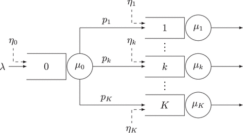
Regular jobs enter the systems only through buffer 0, as shown by the solid arrow pointing to buffer 0 in Figure 1. A renewal process models the cumulative number of regular jobs arriving to the system over time. We let denote the arrival rate and denote the squared coefficient of variation of the interarrival times for the regular jobs. The thin-stream jobs arrive to buffer k (as shown by the dashed arrows in Figure 1) according to the renewal process for . We let denote the arrival rate and denote the squared coefficient of variation of the interarrival times for renewal process .
Jobs in buffer k have i.i.d. general service time distributions with mean and squared coefficient of variation ; is the corresponding service rate. We let denote the renewal process associated with the service completions by server k for . To be specific, denotes the number of jobs server k processes by time t if it incurs no idleness during [0, t]. The jobs in each buffer are served on a first come, first served basis, and servers work continuously unless their buffer is empty. After receiving service, jobs in buffer 0 join buffer k with probability , independently of other events. This probabilistic routing structure is captured by a vector-valued process , where denotes the total number of jobs routed to buffer k among the first jobs served by server 0 for and . We let denote the K-dimensional vector of routing probabilities. Jobs in buffers leave the system upon receiving service.
As stated earlier, the system manager makes admission control decisions for thin-stream jobs. Turning away a thin-stream job arriving to buffer k (externally) results in a penalty of . For mathematical convenience, we model admission control decisions as if the system manager can simply “turn off” each of the thin-stream arrival processes as desired. In particular, we let denote the cumulative amount of time that the (external) thin-stream input to buffer k is turned off during the interval [0, t]. Thus, the vector-valued process represents the admission control policy. Similarly, we let denote the cumulative amount of time that server k is busy during the time interval [0, t], and denotes the cumulative amount of idleness that server K incurs during [0, t].
Letting denote the number of jobs in buffer k at time t, the vector-valued process will be called the queue-length process. Given a control , assuming , it follows that
Moreover, the following must hold:
The system manager also incurs a holding cost at rate per job in buffer k per unit of time. We use the processes as a proxy for the cumulative cost under a given admission control policy where
This is an approximation of the realized cost because the first term on the right-hand side replaces the admission control penalties actually incurred with their means.
In order to derive the approximating Brownian control problem, we consider a sequence of systems indexed by a system parameter we attach a superscript of n to various quantities of interest. Following the approach used by Ata (2006), we assume that the sequence of systems satisfies the following heavy traffic assumption.
For we have that
where , and are nonnegative constants. Moreover, we assume that
One starts the approximation procedure by defining suitably centered and scaled processes. For we define
In what follows, we assume
Then, defining
Moreover, it follows from Equation (71) that is absolutely continuous. We denote its density by
Then, passing to the limit formally as and denoting the weak limit of by where is a -dimensional driftless Brownian motion with covariance matrix (see Appendix C for its derivation)
In order to streamline the notation, we make the following change of variables:
Lastly, we define the set of negative drift vectors available to the system manager as in Equation (64). As a result, we arrive at the following Brownian system model:
To minimize technical complexity, we restrict attention to the stationary Markov control policies as done in Section 3. That is, for for some policy function Then, defining , and
6.2.1. Interpreting the Solution of the Drift Control Problem in the Context of the Queueing Network Formulation.
Because the instantaneous cost rate is linear in the control, inspection of the HJB equation reveals that the optimal control is of a bang-bang nature. That is, for all k, t as stated in Equation (66). This can be interpreted in the context of the queueing network displayed in Figure 1 as follows. For , whenever , the system manager turns away the thin-stream jobs arriving to buffer k externally (i.e., she shuts off the renewal process at time t). Otherwise, she admits them to the system. Of course, the optimal policy is determined by the gradient of the value function through the HJB equation, which we solve for using the method described in Section 5.
6.3. Related Example with Quadratic Cost of Control
Çelik and Maglaras (2008) and Ata and Barjesteh (2023) advance formulations where a system manager controls the arrival rate of customers to a queueing system by exercising dynamic pricing. One can follow a similar approach for the feed-forward queueing networks displayed in Figure 1 with suitable modifications (e.g., the dashed arrows also correspond to the arrivals of regular jobs). This ultimately results in a problem of drift control for RBM with the cost of control
6.4. Two Parametric Families of Benchmark Policies
Recall that the optimal policy can be characterized as
6.4.1. The Benchmark Policy for the Main Test Problem.
In our main test problem (see Section 6.1), we have . Therefore, it follows from (80) that for ,
Namely, the optimal policy is of a bang-bang type. Therefore, we consider the following linear boundary policies as our benchmark polices. For ,
In our numerical study, we primarily focus attention on the symmetric case, where
The symmetry allows us to limit the number of parameters needed for the benchmark policy. To be more specific, because of this symmetry, the downstream buffers look identical. As such, we restrict attention to parameter vectors of the following form:
The parameter vector , which is used to determine the benchmark policy for buffer 0, has two distinct parameters: and . In considering the policy for buffer 0, captures the effect of its own queue length, whereas captures the effects of the downstream buffers . We use a common parameter for the downstream buffers because they look identical from the perspective of buffer 0. Similarly, the parameter vector has three distinct parameters: , and , where is used as the multiplier for buffer 0 (the upstream buffer), is used to capture the effect of buffer i itself, and is used for all other downstream buffers. Note that all use the same three parameters , and for . They only differ with respect to the position of (i.e., it is in the position for ).
In summary, the benchmark policy uses five distinct parameters in the symmetric case. This allows us to do a brute-force search via simulation on a five-dimensional grid, regardless of the number of buffers.
6.4.2. The Benchmark Policy for the Test Problem with the Quadratic Cost of Control.
In this case, substituting Equation (79) into Equation (80) gives the following characterization of the optimal policy:
Namely, the optimal policy is affine in the gradient. Therefore, we consider the following affine rate policies as our benchmark polices. For ,
We focus attention on the symmetric case for this problem formulation too. To be specific, we assume
Because of this symmetry, the downstream buffers look identical. As such, we restrict attention to parameter vectors of the following form:
As done for the first benchmark policy above, this particular form of the parameter vectors can be justified using the symmetry as well.
6.5. Parallel-Server Test Problems
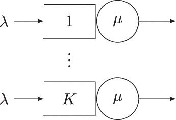
In this section, we consider a problem whose solution can be derived analytically by considering a one-dimensional problem. To be specific, we consider the parallel-server network that consists of K identical single-server queues as displayed in Figure 2. Clearly, this network can be decomposed into K separate single-server queues, leading to K separate one-dimensional problem formulations, which can be solved analytically; see Appendix D for details. For this example, we have that and . In addition, we assume that the action space and the cost function are the same as above.
7. Computational Results
For the test problems introduced in Section 6, we now compare the performance of policies derived using our method (see Section 5) with the best benchmark we could find. The results show that our method performs well, and it remains computationally feasible up to at least dimension . We implement our method using three-layer or four-layer neural networks with the “elu” activation function (Rasamoelina et al. 2020) in Tensorflow 2 (Abadi et al. 2016) and using code adapted from that of Han et al. (2018) and Zhou et al. (2021b); see Appendix E for further details of our implementation.1 In our numerical experiments, we observed that the performance of our method is robust to most hyperparameters. For tuning our algorithm, the activation function proved to be the most critical element. The “elu” activation function resulted in superior performance (Rasamoelina et al. 2020). Additionally, we found that decaying the learning rate to 0.0001 helped achieve good performance.
For our main test problem with the linear cost of control (introduced previously in Section 6.1) and also, for its variant with the quadratic cost of control (Section 6.3), the following parameter values are assumed: , for ; for ; and for . Also, the reflection matrix R and the covariance matrix A for those families of problems are as follows:
We also consider a variation of our main test problem that has asymmetric routing probabilities.
As stated previously in Section 6.5, the reflection matrix and the covariance matrix for our parallel-server test problems are and . Problems in that third class have buffers indexed by , and we set and for .
7.1. Main Test Problem with Linear Cost of Control
For our main test problem with linear cost of control (Section 6.1), we take
Also, interest rates and will be considered in the discounted case.
To begin, let us consider the simple case where (that is, there are no downstream buffers in the queueing network interpretation of the problem), and hence, . In this case, one can solve the HJB equation analytically; see Appendix D for details. For the discounted formulation with , Figure 3 compares the derivative of the value function computed using the analytical solution, which is shown in blue, with the neural network approximation for it that we computed using our method, which shown in red. (The comparisons for and the ergodic control case are similar.)
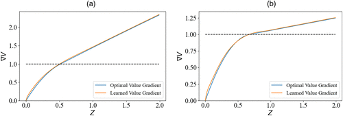
Notes. The dotted lines indicate the cost . When the value function gradient is above the dotted lines, the optimal control is , and otherwise, it is . (a) . (b) .
Combining Figure 3 with Equation (80), one sees that the policy derived using our method is close to the optimal policy. Table 1 reports the simulated performance with standard errors of these two policies based on 4 million sample paths and using the same discretization of time as in our computational method. Specifically, we report the long-run average cost under each policy in the ergodic control case, and we report the simulated value in the discounted case. To repeat, the benchmark policy in this case is the optimal policy determined analytically but not accounting for the discretization of the timescale. Of course, all of the performance figures reported in Table 1 are subject to simulation errors. Finally, it is worth noting that our method took less than one hour to compute its policy recommendations using a 10-CPU core computer.
|

Table 1. Performance Comparison of Our Proposed Policy with the Benchmark Policy in the One-Dimensional Case ()
| Policy | Ergodic | |||
|---|---|---|---|---|
| Our policy | 1.455 0.0006 | 145.3 0.05 | 14.29 0.004 | |
| Benchmark | 1.456 0.0006 | 145.3 0.05 | 14.29 0.004 | |
| Our policy | 1.375 0.0007 | 137.2 0.06 | 13.56 0.005 | |
| Benchmark | 1.374 0.0007 | 137.2 0.06 | 13.56 0.005 |
Let us consider now the two-dimensional case (), where the optimal policy is unknown. Therefore, we compare our method with the best benchmark we could find: the linear boundary policy described in Section 6.4. In the two-dimensional case, the linear boundary policy reduces to the following:
Through simulation, we perform a brute-force search to identify the best values of and . The policies for and are shown in Figures 4 and 5, respectively, for the discounted control case with . Our proposed policy sets the drift to b in the red regions and to zero in the blue regions in Figures 4 and 5, whereas the best linear boundary policy is represented by the white dashed lines in Figures 4 and 5. That is, the benchmark policy sets the drift to b in the region above and to the right of the dashed lines in Figures 4 and 5 and sets it to zero below and to the left of the dashed lines in Figures 4 and 5. Table 2 presents the costs with standard errors of the benchmark policy and our proposed policy obtained in a simulation study. The two policies have similar performance. Our method takes about one hour to compute policy recommendations using a 10-CPU core computer.
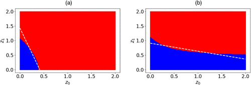
Notes. (a) Server 0. (b) Server 1.
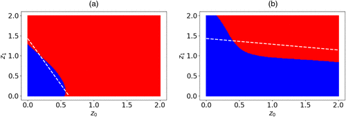
Notes. (a) Server 0. (b) Server 1.
|
Table 2. Performance Comparison of Our Proposed Policy with the Benchmark Policy in the Two-Dimensional Case ()
| Policy | Ergodic | |||
|---|---|---|---|---|
| Our policy | 2.471 0.0008 | 246.6 0.08 | 24.28 0.006 | |
| Benchmark | 2.473 0.0008 | 246.8 0.08 | 24.29 0.006 | |
| Our policy | 2.338 0.0009 | 233.3 0.09 | 23.10 0.006 | |
| Benchmark | 2.338 0.0009 | 233.6 0.09 | 23.10 0.006 |
We then consider the six-dimensional case (), where the linear boundary policy reduces to
Although there appears to be 36 parameters to be tuned, recall that we reduced the number of parameters to 5 in Section 6.4 by exploiting symmetry. This makes the brute-force search computationally feasible. Table 3 compares the performance with standard errors of our proposed policies with the benchmark policies. They have similar performance. In this case, the running time for our method is several hours using a 10-CPU computer.
|
Table 3. Performance Comparison of Our Proposed Policy with the Benchmark Policy in the Six-Dimensional Case ()
| Policy | Ergodic | |||
|---|---|---|---|---|
| Our policy | 7.927 0.001 | 791.0 0.1 | 77.83 0.01 | |
| Benchmark | 7.927 0.001 | 791.3 0.1 | 77.83 0.01 | |
| Our policy | 7.565 0.0016 | 754.8 0.15 | 74.61 0.01 | |
| Benchmark | 7.525 0.0016 | 751.7 0.15 | 74.32 0.01 |
To illustrate the scalability of our approach, we next consider the 21-dimensional case (), where . Because of symmetry, we can perform a brute-force search for the best linear boundary policy as done earlier. The results, presented in Table 4, demonstrate that our method’s performance is comparable with that of the best benchmark. The run time for our method is about one day in this case using a 20-CPU core computer.
|
Table 4. Performance Comparison of Our Proposed Policy with the Benchmark Policy in the 21-Dimensional Case ()
| Policy | Ergodic | |||
|---|---|---|---|---|
| Our policy | 29.12 0.0027 | 2,907 0.26 | 285.8 0.02 | |
| Benchmark | 29.12 0.0027 | 2,907 0.26 | 285.8 0.02 | |
| Our policy | 27.78 0.0031 | 2,773 0.30 | 273.9 0.02 | |
| Benchmark | 27.60 0.0029 | 2,756 0.28 | 272.1 0.02 |
To further demonstrate the effectiveness of our approach, we consider a six-dimensional test problem with asymmetric routing probabilities. Specifically, for the example shown in Figure 1, we set
All other problem parameters remain the same as in the earlier six-dimensional symmetric test problem; see Appendix F for its reflection matrix R and the covariance matrix A. However, for the asymmetric problem, tuning its 36 parameters for the linear boundary policy becomes computationally prohibitive. Therefore, we propose an alternative approach in Appendix F to identify an effective boundary policy. Table 5 presents the performance, along with standard errors, of our proposed policies compared with benchmark policies. The two policies exhibit similar performance, and the run time of our method is comparable with that of the earlier symmetric six-dimensional example.
|
Table 5. Performance Comparison of Our Proposed Policy with the Benchmark Policy in the Six-Dimensional Case () with Asymmetric Routing Probabilities
| Policy | Ergodic | |||
|---|---|---|---|---|
| Our policy | 7.938 0.0013 | 792.5 0.13 | 77.98 0.01 | |
| Benchmark | 7.948 0.0013 | 793.6 0.13 | 78.11 0.01 | |
| Our policy | 7.590 0.0015 | 757.4 0.15 | 74.80 0.01 | |
| Benchmark | 7.547 0.0015 | 753.6 0.15 | 74.53 0.01 |
7.2. Test Problems with Quadratic Cost of Control
In this section, we consider the test problem introduced in Section 6.3, for which we set and for all k. As in the previous treatment of our main test example, we report results for the cases of in Tables 6–8, respectively, where the benchmark policies are the affine rate policies discussed in Section 6.4, with policy parameters optimized via simulation through a brute-force search. We observe that our proposed policies outperform the best affine rate policies by very small margins in all cases.
|
Table 6. Performance Comparison of Our Proposed Policy with the Benchmark Policy in the Case of Quadratic Cost of Control and
| Policy | Ergodic | ||
|---|---|---|---|
| Our policy | 0.757 0.0004 | 75.53 0.03 | 7.415 0.003 |
| Benchmark | 0.758 0.0004 | 75.67 0.03 | 7.427 0.003 |
|
Table 7. Performance Comparison of Our Proposed Policy with the Benchmark Policy in the Case of Quadratic Cost of Control and
| Policy | Ergodic | ||
|---|---|---|---|
| Our policy | 1.216 0.0005 | 121.3 0.04 | 11.94 0.003 |
| Benchmark | 1.219 0.0005 | 121.7 0.05 | 11.96 0.003 |
|
Table 8. Performance Comparison of Our Proposed Policy with the Benchmark Policy in the Case of Quadratic Cost of Control and
| Policy | Ergodic | ||
|---|---|---|---|
| Our policy | 3.863 0.0008 | 385.7 0.08 | 37.92 0.006 |
| Benchmark | 3.874 0.0008 | 386.9 0.08 | 38.04 0.006 |
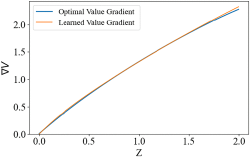
In the one-dimensional ergodic control case (), we obtain analytical solutions to the RBM control problem in closed form by solving the HJB equation directly, which reduces to a first-order ordinary differential equation in this case; see Appendix D for details. Figure 6 compares the derivative of the optimal value function (derived in closed form) with its approximation via neural networks in the ergodic case. Combining Figure 6 with Equation (81) reveals that our proposed policy is close to the optimal policy.
In the two-dimensional case, our proposed policy is shown in Figure 7 for the ergodic case, with contour lines showing the state vectors () for which the policy chooses successively higher drift rates. The white dashed lines in Figure 7 similarly show the states () for which our benchmark policy (that is, the best affine rate policy) chooses the drift rate (for in panel (a) of Figure 7 and in panel (b) of Figure 7).
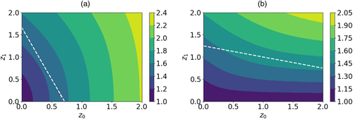
Notes. (a) Server 0. (b) Server 1.
7.3. Parallel-Server Test Problems
This section focuses on parallel-server test problems (see Section 6.5) to demonstrate our method’s scalability. As illustrated in Figure 2, the parallel-server networks are essentially K independent copies of the one-dimensional case. We present the results in Table 9 for and linear cost of control. When , our policies perform almost equally as well as the optimal policy, whereas for , our policies perform within 1% of the optimal policy. The run time for our method is about one day in this case using a 20-CPU core computer.
|
Table 9. Performance Comparison Between Our Proposed Policy and the Benchmark Policy for 30-Dimensional Parallel-Server Test Problems with Linear Cost of Control
| Policy | Ergodic | r = 0.01 | r = 0.1 | |
|---|---|---|---|---|
| Our policy | 42.56 0.003 | 4,247 0.3 | 417.3 0.02 | |
| Benchmark | 42.52 0.003 | 4,244 0.3 | 417.2 0.02 | |
| Our policy | 40.53 0.004 | 4,054 0.4 | 399.4 0.026 | |
| Benchmark | 40.23 0.004 | 4,018 0.4 | 396.7 0.024 |
For quadratic cost of control, we are able to solve the test problems up to at least 100 dimensions. The results for are given in Table 10, where the benchmark policies are the best affine rate policies (see Section 6.4). The performance of our policy is within 1% of the benchmark performance. The run time for our method is several days in this case using a 30-CPU core computer.
|
Table 10. Performance Comparison Between Our Proposed Policy and the Benchmark Policy for 100-Dimensional Parallel-Server Test Problems with Quadratic Cost of Control
| Policy | Ergodic | ||
|---|---|---|---|
| Our policy | 72.74 0.003 | 7,258.3 0.3 | 712.4 0.02 |
| Benchmark | 72.53 0.003 | 7,237.3 0.3 | 710.2 0.02 |
8. Concluding Remarks
Consider the general drift control problem formulated in Section 3, assuming specifically that the instantaneous cost rate is linear in and further assuming that the set of available drift vectors is a rectangle . If one relaxes such a problem by letting for one or more i, then one obtains what is called a singular control problem (cf. Kushner and Martins 1991). Optimal policies for such problems typically involve the imposition of endogenous reflecting barriers (that is, reflecting barriers imposed by the system controller in order to minimize cost) in addition to exogenous reflecting barriers that may be imposed to represent physical constraints in the motivating application.
There are many examples of queueing network control problems whose natural heavy traffic approximations involve singular control; see, for example, Martins and Kushner (1990), Krichagina and Taksar (1992), and Martins et al. (1996). In our follow-up paper (Ata et al. 2024), we extend the method developed in this paper for drift control in a natural way to treat singular control, and we illustrate that extension by means of queueing network applications.
Separately, the following are three desirable generalizations of the problem formulations propounded in Section 3 of this paper. Each of them is straightforward in principle, and we expect to see these extensions implemented in future work, perhaps in combination with mild additional restrictions on problem data. (a) Instead of requiring that the reflection matrix R have the Minkowski form (1), require only that R be a completely matrix, which Taylor and Williams (1993) showed is a necessary and sufficient condition for an RBM to be well defined. (b) Allow a more general state space for the controlled process Z, such as the convex polyhedrons characterized by Dai and Williams (1996). (c) Remove the requirement that the action space be bounded.
Lastly, we have considered in this paper the PDEs that arise in performance analysis and optimal control of RBMs, assuming that those PDEs admit solutions. Borkar and Budhiraja (2005) have established the existence and uniqueness of viscosity solutions for such PDEs, extending the earlier work by Dupuis and Ishii (1991). To the best of our knowledge, there is no theory currently available concerning the existence and uniqueness of classical solutions, either exact or approximate, and we leave that exploration as a topic for future research.
Appendix A. Proof of Proposition 1
Let be right continuous with left limits (rcll). Following Williams (1998a), we define the oscillation of f over an interval as follows:
Also, recall that the controlled RBM Z satisfies , where
Then, it follows from Williams (1998a, theorem 5.1) that
Let , and recall that we are interested in bounding the expectation . To that end, note that
To bound note that
So, by the union bound, we write
Thus,
By change of variable we write
Let We write
Using (A.5), we can, therefore, write
Appendix B. Validity of HJB Equations
B.1. Discounted Control
Let be an admissible policy and be a solution of the associated PDE (15) and (16). If both and its gradient have polynomial growth, then satisfies (12).
Applying Ito’s formula to and using Equation (7), we write
Then, using (3), (4), (15), and (16), we arrive at the following:
Because has polynomial growth and the action space is bounded, we have that
Because has polynomial growth and is bounded, the last term on the right-hand side vanishes as . As mentioned earlier, because is bounded by the assumption, one can easily derive an affine bound for viewed as a function of T. Then, because c has polynomial growth and is bounded, passing to the limit as completes the proof. □
If V is a solution of the HJB Equations (17) and (18) and if both V and its gradient have polynomial growth, then V satisfies (13).
First, consider an arbitrary admissible policy u, and let denote the solution of the associated PDE (15) and (16). By Proposition B.1, we have that
On the other hand, because V solves (17) and (18) and
Now, applying Ito’s formula to and using Equation (7) yields
Combining this with Equations (3), (4), (17), (18), and (B.3) gives
Because has polynomial growth and the action space is bounded, we have that
Because V has polynomial growth and is bounded, the second term on the right-hand side vanishes as . Then, because c has polynomial growth and is bounded, passing to the limit yields
Now, consider the optimal policy , where . For notational brevity, let denote the RBM under policy . Note from Equation (17) that
Repeating the preceding steps with in place of u and replacing the inequality with an equality (cf. Equations (B.3) and (B.7)), we conclude that
Combining this with Equation (B.6) yields (13). □
B.2. Ergodic Control
Let be an admissible policy and be a solution of the associated PDE (24) and (25). Further, assume that and its gradient have polynomial growth. Then,
Let denote the stationary distribution of RBM under policy u, and let denote the RBM under policy u that is initiated with . That is,
Then, applying Ito’s formula to and using Equation (7) yield
Then, using Equations (3), (4), (24), and (25), we arrive at the following:
Note that the marginal distribution of is for all . Thus, we have that
Moreover, using Equation (22) and the polynomial growth of , we conclude that
Consequently, we have that ; see, for example, Oksendal (2003, theorem 3.2.1). Combining these and taking the expectation of both sides of (B.8) gives
Let be a solution of the HJB Equations (26) and (27), and further, assume that both v and its gradient have polynomial growth. Then, (28) holds, and moreover, , where the optimal policy is defined by (29).
First, consider an arbitrary policy u, and note that
On the other hand, because () solves the HJB equation and
Now, we apply Ito’s formula to and use Equation (7) to get
Combining this with Equations (3), (4), (27), and (B.9) gives
Note that the marginal distribution of is for all . Thus, we have that
Moreover, using Equation (22) and the polynomial growth of , we conclude that
Consequently, we have that ; see, for example, Oksendal (2003, theorem 3.2.1). Combining these and taking the expectation of both sides of (B.10) give
Now, consider policy . For notational brevity, let denote the RBM under policy that is initiated with the stationary distribution . In addition, note from (26) that
Repeating the preceding steps with in place of u and replacing the inequality with an equality (cf. Equations (B.9) and (B.12)), we conclude
Combining this with Equation (B.11) completes the proof. □
Appendix C. Derivation of the Covariance Matrix of the Feed-Forward Examples
By the functional central limit theorem for the renewal process (Billingsley 1999), we have
Therefore, the variance of is
In particular, if the arrival and service processes are Poisson processes, we have and for Then, we have
Furthermore, if the service time for server 0 is deterministic (i.e., ), we have
Appendix D. Analytical Solution of One-Dimensional Test Problems
D.1. Ergodic Control Formulation with Linear Cost of Control
We consider the one-dimensional control problem with the cost function
In the ergodic control case, the HJB Equations (26) and (27) are
D.2. Discounted Formulation with Linear Cost of Control
The cost function is still
The solution is
Note that if then we have
Therefore, we have
We have
At point we must have
Then, we can numerically solve for and using the following equations:
Table D.1 presents numerical values of for different parameter combinations.
|
Table D.1. The Numerical Values of for Different Parameter Combinations ()
| h | |||
|---|---|---|---|
| 0.501671 | 0.517133 | ||
| 0.519136 | 0.535753 | ||
| 0.660354 | 0.674135 | ||
| 0.678797 | 0.693707 |
D.3. Ergodic Control Formulation with Quadratic Cost of Control
We consider the cost function
The HJB Equations (26) and (27) then become
Let with Then, we have
Appendix E. Implementation Details of Our Method
Neural network architecture. We used a three-layer or four-layer fully connected neural network with 20–1,000 neurons in each layer; see Tables E.1 and E.2 for details.
|
Table E.1. Hyperparameters Used in the Test Problems with Linear Costs
| Hyperparameters | 1 Dimensional | 2 Dimensional | 6 Dimensional | 30 Dimensional | ||||
|---|---|---|---|---|---|---|---|---|
| b = 2 | b = 10 | b = 2 | b = 10 | b = 2 | b = 10 | b = 2 | b = 10 | |
| No. of iterations | 6,000 | 6,000 | 6,000 | 6,000 | ||||
| No. of epochs | 13 | 17 | 15 | 19 | 23 | 27 | 41 | 135 |
| Learning rate scheme | 0.0005 | (0, 2,000) | 0.0005 | (0, 3,000) | 0.0005 | (0, 3,000) | 0.0005 | (0, 9,500) |
| 0.0003 | (2,000, 4,000) | 0.0003 | (3,000, 6,000) | 0.0003 | (3,000, 6,000) | 0.0003 | (9,500, 22,000) | |
| 0.0001 | (4,000, ) | 0.0001 | (6,000, ) | 0.0001 | (6,000, ) | 0.0001 | (22,000, ) | |
| No. of hidden layers | 4 | 4 | 4 | 3 | ||||
| No. of neurons in each layer | 50 | 50 | 50 | 300 | ||||
| — | — | 0.4 | 7 | 0.4 | 7 | 0.4 | 7 | |
| — | — | 800 | 2,400 | 4,800 | ||||
|
Table E.2. Hyperparameters Used in the Test Problems with Quadratic Costs
| Hyperparameters | 1 Dimensional | 2 Dimensional | 6 Dimensional | 30 Dimensional |
|---|---|---|---|---|
| No. of iterations | 6,000 | 6,000 | 6,000 | 12,000 |
| No. of epochs | 12 | 14 | 22 | 110 |
| Learning rate scheme | 0.0005 (0, 3,000) | 0.0005 (0, 3,000) | 0.0005 (0, 3,000) | 0.0005 (0, 9,500) |
| 0.0003 (3,000, 6,000) | 0.0003 (3,000, 6,000) | 0.0003 (3,000, 6,000) | 0.0003 (9,500, 22,000) | |
| 0.0001 (6,000, ) | 0.0001 (6,000, ) | 0.0001 (6,000, ) | 0.0001 (22,000, ) | |
| No. of hidden layers | 3 | 4 | 4 | 3 |
| No. of neurons in each layer | 20 | 50 | 50 | 1,000 |
Common hyperparameters. Batch size , time horizon , and discretization step size ; see Tables E.1 and E.2 for details.
Learning rate. The learning rate starts from 0.0005 and decays to 0.0003 and 0.0001 with a rate detailed in Tables E.1 and E.2.
Optimizer. We used the Adam optimizer (Kingma and Ba 2014).
Reference policy. The reference policy sets .
Activation function. We use the “elu” action function (Rasamoelina et al. 2020).
Code. Our code structure follows from that of Han et al. (2018) and Zhou et al. (2021b). We implement two major changes. First, we have separated the data generation and training processes to facilitate data reuse. Second, we have conducted the RBM simulation. We have also integrated all of the features discussed in this section.
E.1. Decay Loss in the Test Example with Linear Cost of Control
Recall in our main test example with linear cost of control that the cost function is
In the discounted cost formulation, substituting this cost function into the F function defined in Equation (31) gives the following:
Note that if , we have
We proceed similarly in the ergodic cost case.
E.2. Variance Loss Function in Discounted Control
Let us parametrize the value function as Note that =. Therefore, we can rewrite the loss function (56):
By optimizing first, we obtain the following variance loss function:
We observe that this trick could accelerate the training speed when r is small. Because when is small, is of the order and are of the order .
Appendix F. A Heuristic Approach to Identify an Effective Linear Boundary Policy in Asymmetric Cases
As a preliminary step, we first examine the tandem-queues network depicted in Figure F.1, which can be considered a subnetwork of the queuing network shown in Figure 1.
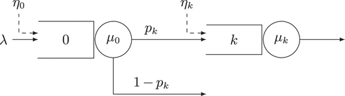
In this system, upon completing their service with server 0, jobs either move on to buffer k with probability or exit the system with probability . Therefore, the reflection matrix associated with the subnetwork is given as follows:
Then, we search for the four parameters for the kth subnetwork to determine the optimal linear boundary policies for each subnetwork (). These policies are represented as
Then, in the original feed-forward queueing network, we set the policies for server as follows:
The reasoning behind this heuristic policy is based on our observations from symmetric cases, indicating that the influence of the length of queue j on the length of queue k is small when j is not equal to zero or k.
In order to complete our specification of the heuristic policy, we search the parameters for server 0 in . In the asymmetric case with , there are four such parameters to tune.
Lastly, for completeness, we provide the reflection matrix R and the covariance matrix A for our test example with asymmetric routing probabilities below:
1 Our code is available at https://github.com/nian-si/RBMSolver.
References
- (2016)
Tensorflow: A system for large-scale machine learning . OSDI, Savannah, GA, vol. 16 (USENIX Association, Berkeley, CA), 265–283.Google Scholar - (1993) Variance reduction through smoothing and control variates for Markov Chain simulations. ACM Trans. Model. Comput. Simulation 3(3):167–189.Google Scholar
- (2006) Dynamic control of a multiclass queue with thin arrival streams. Oper. Res. 54(5):876–892.Link, Google Scholar
- (2023) An approximate analysis of dynamic pricing, outsourcing, and scheduling policies for a multiclass make-to-stock queue in the heavy traffic regime. Oper. Res. 71(1):341–357.Link, Google Scholar
- (2023) Dynamic scheduling of a multiclass queue in the Halfin-Whitt regime: A computational approach for high-dimensional problems. Preprint, submitted November 29, https://arxiv.org/abs/2311.18128.Google Scholar
- (2024) Analysis and improvement of eviction enforcement. Working paper, University of Chicago, Chicago.Google Scholar
- (2005) Drift rate control of a Brownian processing system. Ann. Appl. Probab. 15(2):1145–1160.Google Scholar
- Ata B, Harrison JM, Si N (2024) Singular control of (reflected) Brownian motion: A computational method suitable for queueing applications. Queueing Systems, 1–37.Google Scholar
- (2019) Dynamic volunteer staffing in multicrop gleaning operations. Oper. Res. 67(2):295–314.Abstract, Google Scholar
- (2007) Drift control of international reserves. J. Econom. Dynam. Control 31:3110–3137.Google Scholar
- (2023) An overview on deep learning-based approximation methods for partial differential equations. Discrete Continuous Dynamic. Systems Ser. B 28(6):3697–3746.Google Scholar
- (1999) Convergence of Probability Measures, 2nd ed. (John Wiley & Sons, Hoboken, NJ).Google Scholar
- (2021) Efficient steady-state simulation of high-dimensional stochastic networks. Stochastic Systems 11(2):174–192.Link, Google Scholar
- (2005) Ergodic control for constrained diffusions: Characterization using HJB equations. SIAM J. Control Optim. 43(4):1467–1492.Google Scholar
- (2007) Long time asymptotics for controlled diffusions in polyhedral domains. Stochastic Processes Their Appl. 117(8):1014–1036.Google Scholar
- (2008) Dynamic pricing and lead-time quotation for a multiclass make-to-order queue. Management Sci. 54(6):1132–1146.Link, Google Scholar
- (2022) Queueing network controls via deep reinforcement learning. Stochastic Systems 12(1):30–67.Link, Google Scholar
- (1991) Steady-state analysis of RBM in a rectangle: Numerical methods and a queueing application. Ann. Appl. Probab. 1(1):16–35.Google Scholar
- (1996) Existence and uniqueness of semimartingale reflecting Brownian motions in convex polyhedrons. Theory Probab. Appl. 40(1):1–40.Google Scholar
- (1991) On oblique derivative problems for fully nonlinear second-order elliptic PDEs on domains with corners. Hokkaido Math. J. 20:135–164.Google Scholar
- (2022) Algorithms for solving high dimensional PDEs: From nonlinear Monte Carlo to machine learning. Nonlinearity 35:278–310.Google Scholar
- (2007) Optimal buffer size for a stochastic processing network in heavy traffic. Queueing Systems 55(3):147–159.Google Scholar
- (2010) Optimal buffer size and dynamic rate control for a queueing system with impatient customers in heavy traffic. Stochastic Processes Their Appl. 120(11):2103–2141.Google Scholar
- (2020) Convergence of the deep BSDE method for coupled FBSDEs. Probab. Uncertainty Quantitative Risk 5(1):5.Google Scholar
- (2018) Solving high-dimensional partial differential equations using deep learning. Proc. Natl. Acad. Sci. USA 115(34):8505–8510.Google Scholar
- (1988)
Brownian models of queueing networks with heterogeneous customer populations . Fleming W, Lions PL, eds. Stochastic Differential Systems, Stochastic Control Theory and Applications, The IMA Volumes in Mathematics and Its Applications, vol. 10 (Springer, New York), 147–186.Google Scholar - (2000) Brownian models of open processing networks: Canonical representation of workload. Ann. Appl. Probab. 10(1):75–103.Google Scholar
- (2013) Brownian Models of Performance and Control (Cambridge University Press, Cambridge, UK).Google Scholar
- (1993) Brownian models of multiclass queueing networks: Current status and open problems. Queueing Systems 13:5–40.Google Scholar
- (1981) Reflected Brownian motion on an orthant. Ann. Probab. 9(2):302–308.Google Scholar
- (1989) Scheduling networks of queues: Heavy traffic analysis of a simple open network. Queueing Systems 5:265–279.Google Scholar
- (1990) Scheduling networks of queues: Heavy traffic analysis of a two-station closed network. Oper. Res. 38(6):1052–1064.Link, Google Scholar
- (1987) Brownian models of open queueing networks with homogeneous customer populations. Stochastics 22(2):77–115.Google Scholar
- (2002) Approximating martingales for variance reduction in Markov process simulation. Math. Oper. Res. 27(2):253–271.Link, Google Scholar
- (1998) The vanishing gradient problem during learning recurrent neural nets and problem solutions. Internat. J. Uncertainty Fuzziness Knowledge-Based Systems 6(02):107–116.Google Scholar
- (1970a) Multiple channel queues in heavy traffic. I. Adv. Appl. Probab. 2(1):150–177.Google Scholar
- (1970b) Multiple channel queues in heavy traffic. II. Sequences, networks, and batches. Adv. Appl. Probab. 2(2):355–369.Google Scholar
- (1983) A class of singular control problems. Adv. Appl. Probab. 15(2):225–254.Google Scholar
- (2014) Adam: A method for stochastic optimization. Preprint, submitted December 22, https://arxiv.org/abs/1412.6980.Google Scholar
- (1992) Diffusion approximation for GI/G/1 controlled queues. Queueing Systems 12:333–367.Google Scholar
- (2001) Heavy Traffic Analysis of Controlled Queueing and Communication Networks, Stochastic Modelling and Applied Probability, vol. 28 (Springer, New York).Google Scholar
- (1991) Numerical methods for stochastic singular control problems. SIAM J. Control Optim. 29(6):1443–1475.Google Scholar
- (1990) Routing and singular control for queueing networks in heavy traffic. SIAM J. Control Optim. 28(5):1209–1233.Google Scholar
- (1996) Heavy traffic convergence of a controlled, multiclass queueing system. SIAM J. Control Optim. 34(6):2133–2171.Google Scholar
- (2003) Stochastic Differential Equations: An Introduction with Applications, 6th ed. (Springer Science & Business Media, New York).Google Scholar
- (2011) Drift control with changeover costs. Oper. Res. 59(2):427–439.Link, Google Scholar
- (1991) A heavy traffic limit theorem for networks of queues with multiple customer types. Math. Oper. Res. 16(1):90–118.Link, Google Scholar
- (2020) A review of activation function for artificial neural network. 2020 IEEE 18th World Sympos. Appl. Machine Intelligence Informatics (SAMI) (IEEE, Piscataway, NJ), 281–286.Google Scholar
- (1984) Open queueing networks in heavy traffic. Math. Oper. Res. 9(3):441–458.Link, Google Scholar
- (2009) Dynamic control of a make-to-order, parallel-server system with cancellations. Oper. Res. 57(1):94–108.Link, Google Scholar
- (1993) Existence and uniqueness of semimartingale reflecting Brownian motions in an orthant. Probab. Theory Related Fields 96(3):283–317.Google Scholar
- (2021) Average cost Brownian drift control with proportional changeover costs. Stochastic Systems 11(3):218–263.Link, Google Scholar
- (1991) Brownian networks with discretionary routing. Oper. Res. 39(2):322–340.Link, Google Scholar
- (1996) On the approximation of queueing networks in heavy traffic. Stochastic Networks Theory Appl. 4:35–56.Google Scholar
- (1998a) An invariance principle for semimartingale reflecting Brownian motions in an orthant. Queueing Systems 30:5–25.Google Scholar
- (1998b) Diffusion approximations for open multiclass queueing networks: Sufficient conditions involving state space collapse. Queueing Systems 30:27–88.Google Scholar
- (2012) Moments and absolute moments of the normal distribution. Preprint, submitted September 19, https://arxiv.org/abs/1209.4340.Google Scholar
- (2020) Wasserstein control of mirror Langevin Monte Carlo. Conf. Learn. Theory (PMLR, New York), 3814–3841.Google Scholar
- (2021a) Actor-critic method for high dimensional static Hamilton–Jacobi–Bellman partial differential equations based on neural networks. SIAM J. Sci. Comput. 43(6):A4043–A4066.Google Scholar
- (2021b) Code for “Actor-critic method for high dimensional static Hamilton–Jacobi–Bellman partial differential equations based on neural networks.” https://github.com/MoZhou1995/DeepPDE_ActorCritic.Google Scholar