Exponential Single Server Queues in an Interactive Random Environment

1. Introduction and Literature Review

Queueing systems that evolve under influences from external sources have found interest for long times. Today’s emerging complex technological and logistic systems revived interest in such models. Features of interest in these systems are, for example, services of different quality that are provided to individual customers, or to general differentiated demand, or even to data sets (messages in sensor networks), etc., under side-constraints of limited and shared resources and under restrictions that are external from the point of view of the service system. The need for understanding the behavior of these systems revived investigations of queueing systems in a dedicated environment. Because in real life situations service systems are subject to randomness of interarrival times and service time requests, and environments are usually nondeterministic, the area of queues in random environments is today a field of active research in applied probability.

1.1. Problem Setting

The model of a queue in a random environment studied in this note summarizes and unifies various models that emerged over the last two decades in different research areas, especially in Operations Research. The following standard example of a production-inventory system will serve as an introductory example and will be modified in course of the article.

Example 1

(Production-Inventory System, see Figure 1). The production system with an attached inventory considered here fits into the class of queueing systems in a random environment: The production system ($=$ exponential server) interacts with an inventory and an associated replenishment system (supplier) (environment $=$ inventory-replenishment subsystem).

The production system consists of a single server (machine) with infinite waiting room that serves demand of customers on a make-to-order basis under first-come-first-served regime (FCFS). To satisfy a customer’s demand the production system needs exactly one item of raw material from the associated inventory.

Arriving customers join the queue unless the inventory is depleted ($=$ “lost sales” principle from inventory theory). If customers are present and the inventory is not depleted, the customer at the head of the line is served and new arrivals are admitted. A customer departs from the system immediately after service and the associated consumed raw material is formally removed from the inventory at this instant of time. If the server is ready to serve a customer and the inventory is not depleted, service immediately starts. Otherwise, customers in the waiting line stay on and service starts again when the next replenishment arrives.

The main characteristic of the production-inventory system is in our setting the following: If the inventory is depleted, no service is possible and new arrivals are lost. A sketchy formal description of the queueing-environment interaction in this example is as follows. (More information will be given in Example 2.)

The production system is modelled as a standard exponential queueing system with state space ${\mathbb{N}}_0$ (queue lengths) and the inventory with state space $K≔\{0,1,\dots ,b\}$ (inventory sizes) is its environment, which influences the queue’s development. The decisive properties for our class of models are: (i) Whenever the state of the inventory is in the subset $K_W≔\{1,\dots ,b\}\subseteq K$, the queue is functioning properly (Works), service and arrival processes are ongoing. (ii) Whenever the state of the inventory is in the subset $K_B≔\{0\}\subseteq K$, the queueing system is completely stalled (Blocked) (due to stock-out no production can be performed and because of the lost sales regime no new arrivals occur).

An important property of the system’s dynamics is that neither the queue nor the inventory evolves autonomously. The production system can only serve if the inventory is not depleted (stock size > 0), and the inventory can only decrease whenever production is possible (queue length > 0). We characterize this as a “bidirectional interaction.” Note that the replenishment system is part of the environment, although it is only implicitly represented in K.

1.2. Literature Review

1.2.1. Queues in a Random Environment.

A recent review of queueing-inventory systems (as in Example 1) is the article of Krishnamoorthy et al. (2019), including 10 pages of references. The majority of the articles mentioned in this review is on nonseparable systems, but separable queueing-inventory systems in the spirit of our investigations are compiled and discussed as well.

We observed that the dichotomy K_B versus K_W, that is, a partition of K occurs with many very different queueing models. Representative examples are as follows:

1. Supply chains of production facilities (modelled as a queue) with an attached inventory as described in Example 1. This model was investigated first in the articles of Sigman and Simchi-Levi (1992) and Melikov and Molchanov (1992), where demand in case of stock-out at the inventory is backordered. Intensive research on this model started with a series of articles by Berman and his coauthors, for example, Berman and Kim (1999), Berman and Sapna (2000, 2002). The first explicit result on stationary behavior for such integrated production-inventory models is developed by Schwarz et al. (2006), where demand in case of stock-out at the inventory is lost. It was shown that the associated queueing-inventory process is separable. A review of separable queueing-inventory systems is the article of Krishnamoorthy et al. (2011). More contributions that focus on product form steady states are the articles of Saffari et al. (2011, 2013) and the theses of Vineetha (2008) and Otten (2018).

2. Sensor networks, where a dedicated node (test node, referenced node) featuring an internal message queue that interacts with a complex environment. The environment incorporates location and status of neighbored sensor nodes and geographical conditions, as well as internal status information of the referenced node, for example, activity level or sleep mode. Here K_B consists of those environmental states that indicate (among other properties of the system) that the referenced node is sleeping and can neither receive, process, or forward messages. K_W encompasses all other environment states and if the environment is in such state, the dedicated node’s message queue is functioning properly. A detailed study is given by Krenzler and Daduna (2014), where a compilation of related literature can be found in section 1.

3. Queues where the availability of service capacity depends on external conditions and/or control decisions. These external conditions are collected in the environment set K and the subset K_B consists of those states where the server is stalled, for example, for preventive maintenance. This has been researched for decades; see a review in Krishnamoorthy et al. (2014). Explicit formulas for the stationary distribution of such systems were derived by Sauer and Daduna (2003). A recent study of performability for a randomly degrading queue with maintenance options in the spirit of our present research is the article of Krenzler and Daduna (2015b).

4. Queueing networks, where a node of special interest is embedded in the environment set K constituted by the set of the other nodes, are investigated by van Dijk (1993, section 4.5.1) and Krenzler and Daduna (2015a, section 4.2.2). In a network with finite buffers, a typical example of a state in K_B is defined by those states where the other nodes have full buffers and the node of special interest is therefore stalled.

5. Queues in a random environment as an example for application of matrix-analytical methods in the framework of quasi-birth-death processes (QBDs). Typical examples are Markov-arrival processes (MAPs) with queue-length-dependent service mechanisms and related structures; see, for example, Neuts (1981, sections 3 and 6) for general principles. A control problem for queues in a random environment is investigated by Helm and Waldmann (1984). The common feature of all these quasi-birth-death process models is the following: The queue length process is the level process while the environment process is the phase process. It will become obvious that our systems can be formulated as QBDs, but most of the other mentioned QBDs do not obey the dichotomy K_W versus K_B for the states in the environment space K. A note in the spirit of the present article is by Economou (2003) where criteria for the existence of a stationary distribution of product form are provided.

6. Closely related to our present research on queues subject to external side-constraints with accessible stationary distribution are the articles of Falin (1996) and Krenzler and Daduna (2015a).

1.2.2. Related Models.

A Markovian exponential queueing-environment process can be considered as birth-death process in a random environment. There exists a bulk of literature on that subject. Classical birth-death processes (with discrete or continuous time) in a random environment found in the literature are not separable. We discuss some examples shortly. Discrete time Markov chains in a Markovian random environment are investigated by Cogburn (1980, 1984). In the first paper classification of states are provided and in the second conditions for the existence of stationary distributions and for ergodicity are presented. Cornez (1987) investigated a discrete time birth-death process with absorbing state 0 in a general environment with feedback (bidirectional interaction); Cogburn and Torrez (1981) investigated continuous time birth-death processes in a Markovian random environment and provide criteria for recurrence and transience. Applications to queues in a Markovian environment are sketched. Yechiali (1973) considered continuous time birth-death processes in a finite ergodic Markovian environment. The birth and death rates depend on the environment state and the population size. The focus is on stationary regime and it is shown that “in general, closed-form results for the limiting probabilities are difficult to obtain” (Yechiali 1973, p. 604). For population size independent birth-death rates, a special condition is found that allows to obtain geometrical steady state distribution. Prabhu and Zhu (1989, 1995) investigated single server systems under Markov-modulation (which is similar to a Markovian environment). In the first paper, the modulated Poissonian arrival stream generates single customer arrivals, while in the second paper group arrivals are considered. The focus is on stationary behavior.

Typical problems with computing stationary distributions and performance metrics that occur even with finite (nonseparable) birth-death processes in a random environment are described in Gaver et al. (1984) and investigated using matrix-analytical techniques.

In Gannon et al. (2016) a reversible Jacksonian queueing network is the environment for a random walker (a distinguished customer) on the network lattice. This work was extended in Daduna (2016), where the random walker was substituted by a travelling server (“moving queue”) on the network. This was motivated by modeling a referenced mobile sensor node with an internal message queue (test node) in a network of mobile sensor nodes. Although the stationary distributions occurring in Daduna (2016) are separable, the transition mechanism of the system does not fit in the class of models considered here in Section 3.

A recent study of an $M/M/1$-queue in abstract “interactive” environments is the article of Pang et al. (2020), where the environment is either diffusive (continuous environment space) or a jump environment (discrete environment space). We consider only discrete environment spaces. Our systems and processes differ from those in Pang et al. (2020, section 2) because we allow (i) that the arrival and service rates are queue-length-dependent, and (ii) that the queueing system and the environment may jump concurrently. Recall that in Example 1 with departures of served customers the environment ($=$ inventory size) decreases at the same moment by one. Such concurrent jumps are not allowed by Pang et al. (2020). On the other side, the dependence on the environment’s state for the arrival and service rates are more specific in our setting.

A related class of models are random walks on $\mathbb{Z}$ in a random medium, see Part I of Sznitman (2002) for an introduction. Our research in this article is on different problems than those described there and our methods are different from those used generally in that field.

1.3. Research Plan

We are interested in a unified Markovian description for a class of general queueing-environment systems. The above examples reveal general principles: (i) The environment state space K is divided into disjoint subsets: K_W and K_B. (ii) The evolution of the system follows general rules but in any case some special environment conditions, modelled as states in K_B interrupt the dynamics of the queueing system, and the server is stalled as long as these conditions hold on. (iii) The environment is nonautonomous with respect to the queueing system, that is, its dynamics depend on the status of the associated queue. This bidirectional interaction is different from most work in the literature but reflects many real situations, as shown in examples above. (iv) Concurrent jumps of the queue and the environment occur with positive probability.

Special emphasis will be put on

• separable models with product form steady state: Asymptotically and in equilibrium the queue and the environment as components (in space) of the one-dimensional marginals in time decouple. (In steady state the queue and the environment seem to behave independently at fixed times.) This usually allows to determine ergodicity conditions directly, and

• nonseparable models where ergodicity and exponential ergodicity conditions via construction of Lyapunov functions will be proven. In this case the infinite system of global balance equations of the joint queueing-environment process are usually not explicitly solvable.

The environment is always modelled by a discrete state space. In Sections 2, 3, 4, and 5.1, the environment is allowed to be infinite, from Section 5.2 on we assume the environment to be finite.

1.4. Main Results and Techniques

• (i) We identify a large class of separable queues with finite or infinite waiting room in a nonautonomous random environment. We compute explicitly the stationary distribution, which opens the path for performance evaluation of these systems. The main part of the proof is to substitute the two-dimensional set of global balance equations by a set of independent one-dimensional equations with the same solution. This is combined with the stationary distribution of the isolated queue, which is well known.

• (ii) For nonseparable systems we provide necessary conditions for ergodicity, which reveal a hidden geometrical structure of the (unknown) stationary distribution. Sufficient criteria for ergodicity and exponential ergodicity are proved using a Lyapunov function approach. The main technique is to start with an ergodic version of the queue in isolation (which usually can be easily characterized) and an associated Lyapunov function for the queue only. Taking this function as partial function of the two-dimensional target function, a second partial (environment) function is attached to obtain the final function.

• (iii) We take the explicit results of (i) to approximate performance measures of the ergodic (proved via (ii)) nonseparable system (no stationary distribution at hand) using lower and upper bounds of modified versions of the target system, which are separable. The main technique is to construct suitable reward processes, which generate the respective performance measures.

1.4.1. Structure of the Article.

In Section 2 we describe the general model of a queueing system in a nonautonomous random environment. In Section 3 we characterize separability of the queueing-environment process and derive ergodicity conditions and the stationary distribution. The case of a finite waiting room is investigated in Section 4. In Section 5 we investigate nonseparable queueing-environment systems. In Section 5.1 we prove a necessary condition for ergodicity of nonseparable queueing systems in a random environment, which is trivially valid in the separable case. In Section 5.2 we provide sufficient conditions for ergodicity by constructing a Lyapunov function, which indicates negative drift of the queueing-environment process. The section ends with a nonseparable modification of the introductory Example 1. In Section 5.3 we prove conditions for exponential ergodicity. In Section 6 we combine our findings on separable and nonseparable systems by showing that in many cases it is possible to find for a nonseparable system related separable partner systems such that performance indices of the former (which are not explicitly computable) can be bounded by the respective indices of the separable partner.

1.4.2. Notations, Definitions, and Conventions.

• ${\mathbb{R}}_0^{+}≔[0,\infty ),\hspace{0.17em}{\mathbb{R}}^{+}≔(0,\infty ),\hspace{0.17em}\mathbb{N}$:= {1,2,3,…}, ${\mathbb{N}}_0≔\{0\}\cup \mathbb{N}$

• Empty sums are 0, and empty products are 1.

• $1_{\{\mathit{\text{expression}}\}}$ is the indicator function, which is 1 if expression is true and 0 otherwise.

• We write $C≔A+B$ to emphasize that C is the union of disjoint sets A and B.

• For $a\in \mathbb{R}$ we set $a_{+}≔\max \{0,a\}$.

• All random variables and processes occurring henceforth are defined on a common underlying probability space $(\mathrm{\Omega },\mathcal{F},P)$.

Queueing systems in a random environment are described in this article by homogeneous Markov processes with countable (discrete) state space. All processes occurring henceforth have the properties summarized in the following definition.

Definition 1.

A Markov process X with state space E and transition rate matrix Q is regular if (i) all states are stable, that is, all diagonal elements of Q are finite, and (ii) Q is conservative, that is, its row sums are zero, and (iii) the process is nonexplosive, that is, the sequence of jump times of the process diverges almost surely. X has cadlag paths, that is, each path of X is right-continuous and has left limits everywhere.

The Markov process X is ergodic if there exists a probability measure $\pi ≔(\pi (z):z\in E)$ such that $P(X(t)=z|X(0)=\widehat{z})\to \pi (z)$ for $t\to \infty$ holds for all $z\in E$ independent of the initial state $X(0)=\widehat{z},\hspace{0.17em}\widehat{z}\in E$. π is the asymptotic and stationary distribution of X.

An ergodic Markov process X with asymptotic distribution π is exponentially ergodic if there exists some $\alpha >0$ and constants $C_{z,\widehat{z}}>0,z,\widehat{z}\in E,$ such that $|P(X(t)=z|X(0)=\widehat{z})-\pi (z)|\le C_{z,\widehat{z}}·e^{-\alpha ·t}$ for all $z,\widehat{z}\in E$ holds.

We use the following Foster-Lyapunov criteria for ergodicity (see Kelly and Yudovina 2014, proposition D.3) and exponential ergodicity (see Anderson 1991, theorem 6.5).

Proposition 1.

Let $X≔(X(t):t\ge 0)$ be an irreducible regular Markov process with countable state space E and transition rate matrix $\mathbf{Q}≔(q(x;y):x,y\in E)$. Suppose that $\mathcal{L}:E\to [0,\infty )$ is a function such that for constants $\epsilon >0$ and $b\in \mathbb{R}$, and some finite exception set $F\subset E$ and all $x\in E$ it holds

$${\displaystyle \sum _{y\in E\setminus \{x\}}q}(x;y)[\mathcal{L}(y)-\mathcal{L}(x)]\le \{\begin{array}{ll}-\epsilon \hfill & x\notin F,\hfill \\ b-\epsilon \hfill & x\in F.\hfill \end{array}$$(1)

Then X is ergodic.

Proposition 2.

Let $X≔(X(t):t\ge 0)$ be an ergodic Markov process with countable state space E and transition rate matrix $\mathbf{Q}≔(q(x;y):x,y\in E)$. X is exponentially ergodic if and only if there exists a function $\mathcal{M}:E\to [0,\infty )$, a finite exception set $F\subset E$, and some $\omega \in (0,{\inf }_{x\in E\setminus F}(-q(x;x)))$ such that the following holds:

$$\mathcal{M}(x)=0, x\in F,$$(2)

$${\displaystyle \sum _{y\in E}q}(x;y)\mathcal{M}(y)<\infty , x\in F,$$(3)

$${\displaystyle \sum _{y\in E\setminus \{x\}}q}(x;y)[\mathcal{M}(y)-\mathcal{M}(x)]\le -\omega \mathcal{M}(x)-1, x\in E\setminus F.$$(4)

The functions $\mathcal{L}$ and $\mathcal{M}$ in the above propositions are called drift functions or Lyapunov functions. In the literature, Lyapunov functions are utilized as test functions to prove other properties of Markov processes (explosion, nonexplosion, absorption) as well. Usually the processes’ behavior, especially the drift, is characterized via transformation of the test functions by the infinitesimal generator.

2. The Model: Queue in an Interactive Random Environment

Our starting point is the classical M/M/1/$\infty$-queue with queue-length-dependent rates under first-come-first-served regime (FCFS). Customers are indistinguishable. If the queue length (i.e., number of customers either waiting or in service) is $n\ge 0$, customers arrive at the system with rate $\lambda (n)>0,$ and if $n\ge 1$, service is provided to the customer at the head of the line with rate $\mu (n)>0$. We set formally $\mu (0)≔0$.

Setting in force the usual (conditional) independence assumptions, the queue length process $X≔(X(t):t\ge 0)$ with state space ${\mathbb{N}}_0$ is Markov. It is the simplest example of a birth-death process, which in case of ergodicity has stationary distribution $\xi ≔(\xi (n):n\in {\mathbb{N}}_0)$ with

where C is the normalization constant.

We consider the situation where the service system and the arrival stream are subject to external random influences that disturb the queueing process; see Figure 2. The states of the environment are summarized as countable environment state space $K\ne Ø$ and the environment process is denoted by $Y≔(Y(t):t\ge 0)$. The joint queueing-environment process is $Z≔(X,Y)=((X(t),Y(t)):t\ge 0)$ on state space $E≔{\mathbb{N}}_0\times K$, that is, $Z(t)≔(X(t),Y(t))=(n,k)$ indicates that at time t the queue length is n and the environment’s state is k.

In most investigations found in the literature (e.g., Zhu (1994), Economou (2005), Foss et al. (2012)) an autonomous environment is considered: This means that the environment process $Y=(Y(t):t\ge 0)$ on K is Markov of its own, and the state of the environment influences arrival and service rates of the queue. Consequently, in this situation there is only a “one-way interaction.”

We consider in this note mainly the case of nonautonomous environments: Then the environment process Y on K is not Markov of its own. The state of the environment and state of the queue influence transitions of the other component of the system vice-versa, which results in a “two-way interaction.” In case of birth-death processes in a random environment, this is often termed “feedback property of the environment”; see, for example, Cornez (1987).

In all applications mentioned in the introduction, for the joint queueing-environment process $Z=(X,Y)$ on $E={\mathbb{N}}_0\times K$ we observe that the environment space K is partitioned as a disjoint union $K=K_W+K_B$ with the following meaning and consequences:

• $Y(t)\in K_B$ $:\iff$ at time t no service is provided and no arrivals occur; that is, the queue length process X is frozen (= server is Blocked).

• $Y(t)\in K_W$ $:\iff$ at time t the server is functioning, new arrivals are admitted (= server Works).

The dynamics of the environment are as follows: If the queue length is $n\in {\mathbb{N}}_0$, then

• a generator $V_n≔(v_n(k,m):k,m\in K)$ governs continuous changes of the environment for $n\ge 0,$ and

• a stochastic matrix $R_n≔(r_n(k,m):k,m\in K)$ governs instantaneous jumps of the environment triggered by service completions (downward jumps of the queue) for $n\ge 1$.

We henceforth assume that $Z=(X,Y)=((X(t),Y(t)):t\ge 0)$ is a Markov process on $E={\mathbb{N}}_0\times K$. The characterizing data for the system’s development are $\lambda (n),\hspace{0.17em}\mu (n)$, the countable environment $K=K_W+K_B$, and the driving components for the environment R_n and V_n. The generator $\mathbf{Q}≔(q(z,\tilde{z}):z,\tilde{z}\in E)$ of Z is with generic state $(n,k)\in E$:

and $q(z;\tilde{z})≔0$ for other $z\ne \tilde{z}$, and $q(z;z)≔-{\sum }_{\stackrel{\tilde{z}\in E,}{z\ne \tilde{z}}}q(z;\tilde{z})$ for all $z\in E.$

We note that such processes can be considered as quasi-birth-death processes with level-dependent phase-dynamics.

As pointed out in Section 1 the class of Markov processes $Z=(X,Y)$ on $E={\mathbb{N}}_0\times K$ with generator given by (6) encompasses a rich class of examples from different application areas. The typical examples lead to Markov processes Z, which are irreducible on E. On the other side, the general construction (6) allows examples of reducible systems, which seem to be of no specific interest. We therefore set in force the following assumption.

Assumption 1.

We assume throughout that $Z=(X,Y)$, resp. Q is irreducible on E.

Remark 1.

Although $Z=(X,Y)$ is a Markov process, neither X nor Y is in general Markov. Moreover, even under Assumption 1 neither the R_n nor the V_n need to be irreducible nor determines an ergodic Markov chain, respectively an ergodic Markov process.

3. Separable Queueing-Environment Systems

Separability means roughly that the state vector of a multidimensional Markov process in equilibrium has for a fixed moment independent coordinates. The classical examples are Jackson networks of queues (Jackson 1957) and their generalizations as BCMP networks (Baskett et al. 1975), resp. Kelly networks (Kelly 1976). We are interested in conditions that guarantee this asymptotic (resp. equilibrium) independence for the pair $Z=(X,Y)$. A characterization theorem for the case when the dynamics of the environment are independent of queue lengths, that is, V_n = V, R_n = R for all n, is proved in Krenzler and Daduna (2012, theorem 2). We provide a characterization for the general case here.

Theorem 1.

• (a) For $n\in {\mathbb{N}}_0$ define “reduced generators” ${\mathbf{Q}}_{\mathit{\text{red}}}^{(n)}≔(q_{\mathit{\text{red}}}^{(n)}(k,m):k,m\in K)$ on the environment space K via Q by

  $$q_{\mathit{\text{red}}}^{(n)}(k,m)≔\lambda (n)·r_{n+1}(k,m)·1_{\{k\in K_W\}}+v_n(k,m),\hspace{1em}\hspace{1em}k\ne m,$$
  $$q_{\mathit{\text{red}}}^{(n)}(k,k)≔-[1_{\{k\in K_W\}}·\lambda (n)·(1-r_{n+1}(k,k))+\sum _{m\in K\backslash \{k\}}{v}_n(k,m)].$$

  The reduced generators ${\mathbf{Q}}_{\mathit{\text{red}}}^{(n)}$ are generators for Markov processes on K.

• (b) The following properties are equivalent:

  • (i) $Z=(X,Y)$ is ergodic with product form steady state $\pi =\xi ·\theta$, with $\xi ≔(\xi (n):n\in {\mathbb{N}}_0)$ from (5), that is,

    $$\pi (n,k)=C^{-1}·\left({\displaystyle \prod _{i=0}^{n-1}\frac{\lambda (i)}{\mu (i+1)}}\right)·\theta (k),\hspace{1em}(n,k)\in E,$$(7)
    where $\theta ≔(\theta (k):k\in K)$ is a probability distribution on K.

  • (ii) The summability condition $C≔{\sum }_{n=0}^{\infty }{\prod }_{i=0}^{n-1}\frac{\lambda (i)}{\mu (i+1)}<\infty$ holds, and the equation

    $$\theta ·{\mathbf{Q}}_{\mathit{\text{red}}}^{(0)}=0$$(8)
    admits a strictly positive stochastic solution $\theta ≔(\theta (k):k\in K)$ which solves also
    $$\forall n\in \mathbb{N}:\theta ·{\mathbf{Q}}_{\mathit{\text{red}}}^{(n)}=0.$$(9)

Proof.

(a) Let $k\in K$. By definition we have $q_{\mathit{\text{red}}}^{(n)}(k,m)\ge 0$ for all $m\in K\setminus k$ and $q_{\mathit{\text{red}}}^{(n)}(k,k)\le 0.$ It holds

$$\begin{array}{l}{\displaystyle \sum _{m\in K\setminus \{k\}}{q}_{\mathit{\text{red}}}^{(n)}}(k,m)={\displaystyle \sum _{m\in K\setminus \{k\}}(\lambda (n)·r_{n+1}(k,m)·1_{\{k\in K_W\}}+v_n(k,m))}\hfill \\ =\lambda (n)·1_{\{k\in K_W\}}\underset{=1-r_{n+1}(k,k)}{\underbrace{{\displaystyle \sum _{m\in K\setminus \{k\}}{r}_{n+1}}(k,m)}}+{\displaystyle \sum _{m\in K\setminus \{k\}}{v}_n}(k,m)=-q_{\mathit{\text{red}}}^{(n)}(k,k).\hfill \end{array}$$

So the row sums of all ${\mathbf{Q}}_{\mathit{\text{red}}}^{(n)},n\in {\mathbb{N}}_0,$ are zero.

(b) (ii) $\Rightarrow$ (i): By assumption (8) there exists a stochastic solution to $\theta ·{\mathbf{Q}}_{\mathit{\text{red}}}^{(0)}=0$, which according to requirement (9) is a solution of $\theta ·{\mathbf{Q}}_{\mathit{\text{red}}}^{(n)}=0$ too. Due to the summability condition $C<\infty$, we can use our θ and C to define $\pi (n,k)$ by the right-hand side of (7). Next, we show that π fulfills the global balance equation $\pi ·\mathbf{Q}=\mathbf{0}$ of the Markov process (X,Y), which are for $(n,k)\in E$

$$\begin{array}{lll}\hfill & \hfill & \pi (n,k)·(1_{\{k\in K_W\}}·\lambda (n)+\sum _{m\in K\backslash \{k\}}{v}_n(k,m)+1_{\{k\in K_W\}}·1_{\{n>0\}}·\mu (n))\hfill \\ \hfill & =\hfill & \pi (n-1,k)·1_{\{k\in K_W\}}·1_{\{n>0\}}·\lambda (n-1)+{\displaystyle \sum _{m\in K_W}\pi }(n+1,m)·r_{n+1}(m,k)·\mu (n+1)\hfill \\ \hfill & \hfill & +\sum _{m\in K\backslash \{k\}}\pi (n,m)·v_n(m,k).\hfill \end{array}$$(10)

Inserting the proposed product form solution (7) for the stationary distribution into the global balance Equation (10), canceling $C^{-1}$ and multiplying with ${\prod }_{i=0}^{n-1}{(\lambda (i)/\mu (i+1))}^{-1}$ yields

$$\begin{array}{lll}\hfill & \hfill & \theta (k)·(1_{\{k\in K_W\}}·\lambda (n)+\sum _{m\in K\backslash \{k\}}{v}_n(k,m)+\underset{(*)}{\underbrace{1_{\{k\in K_W\}}·1_{\{n>0\}}·\mu (n)}})\hfill \\ \hfill & =\hfill & \underset{(**)}{\underbrace{\theta (k)·\frac{\mu (n)}{\lambda (n-1)}·1_{\{k\in K_W\}}·1_{\{n>0\}}·\lambda (n-1)}}+{\displaystyle \sum _{m\in K_W}\theta }(m)·\frac{\lambda (n)}{\mu (n+1)}·r_{n+1}(m,k)·\mu (n+1)\hfill \\ \hfill & \hfill & +\sum _{m\in K\backslash \{k\}}\theta (m)·v_n(m,k).\hfill \end{array}$$

Canceling for $n\ge 1$ the expressions $(\theta (k)·(*))$ and $(**)$ yields for all $n\ge 0$

$$\begin{array}{lll}\hfill & \hfill & \theta (k)·(1_{\{k\in K_W\}}·\lambda (n)+\sum _{m\in K\backslash \{k\}}{v}_n(k,m))\hfill \\ \hfill & =\hfill & {\displaystyle \sum _{m\in K_W}\theta }(m)·\lambda (n)·r_{n+1}(m,k)+\sum _{m\in K\backslash \{k\}}\theta (m)·v_n(m,k).\hfill \end{array}$$

This implies

$$\begin{array}{lll}\hfill & \hfill & \theta (k)·\underset{=-q_{\mathit{\text{red}}}^{(n)}(k,k)}{\underbrace{(1_{\{k\in K_W\}}·\lambda (n)·(1-r_{n+1}(k,k))+\sum _{m\in K\backslash \{k\}}{v}_n(k,m))}}\hfill \\ \hfill & =\hfill & {\displaystyle \sum _{m\in K\setminus \{k\}}\theta }(m)·\underset{=q_{\mathit{\text{red}}}^{(n)}(m,k)}{\underbrace{\left(1_{\{m\in K_W\}}·\lambda (n)·r_{n+1}(m,k)+v_n(m,k)\right)}},\hfill \end{array}$$(11)

which is for all $n\ge 0$ the condition (8), respectively (9), that is, $\theta ·{\mathbf{Q}}_{\mathit{\text{red}}}^{(n)}=0$. Hence, we conclude that (8) and (9) guarantee that (7) solves (10). Therefore, the global balance equations of Z admit the strictly positive stochastic solution $\pi =\xi ·\theta$, which is unique by Assumption 1, and so Z is ergodic.

(b) (i) $\Rightarrow$ (ii): Because π is stochastic and of product form, summability holds. Insert the stochastic vector of product form (7) into (10). As shown in the part (ii) $\Rightarrow$ (i) of the proof, this leads to (11) and we have found a strictly positive stochastic solution θ, which solves (8) and (9) for all $n\in \mathbb{N}$. □

Remark 2.

The reduced generators ${\mathbf{Q}}_{\mathit{\text{red}}}^{(n)}=(q_{\mathit{\text{red}}}^{(n)}(k,m):k,m\in K)$ can be considered as generalizations of the generators ${\mathbf{T}}_n,n\in {\mathbb{N}}_0,$ in the construction of the Markovian jump generators in Pang et al. (2020, section 2). The reduced generators ${\mathbf{Q}}_{\mathit{\text{red}}}^{(n)}$ enable concurrent jumps in two dimensions for the original generator Q. The property that θ is the common solution of the Equations (8) and (9) is parallel to Assumption 2.1 in Pang et al. (2020) required for the ${\mathbf{T}}_n,n\in {\mathbb{N}}_0,$ there.

Example 2

(Production-Inventory System, See Example 1 with Figure 1). As described in the introduction, this production-inventory system fits into the definition of the queueing system in a random environment described by a Markov process $Z=(X,Y)=(\text{queue-length},\hspace{0.17em}\text{inventory}\hspace{0.17em}\text{size})$ on state space $E={\mathbb{N}}_0\times K$ with $K≔\{0,1,\dots ,b\}$ and

$$K_B≔\{0\},\hspace{1em}\hspace{1em}{K}_W≔\{1,\dots ,b\}.$$

$Y(t)\in K_W$ indicates for the inventory that there is stock on hand for production, and $Y(t)\in K_B$ indicates stock-out.

The inventory is controlled according to the base stock policy, that is, each item taken from the inventory triggers an immediate order for one item of raw material at the supplier. The base stock level $b\ge 1$ is the maximal size of the inventory. The supplier consists of a single server with waiting room of size b – 1 under FCFS. Service times to produce one item of raw material at the supplier are exponentially distributed with parameter $\nu >0$. A finished item of raw material departs immediately from the supplier and is added to the inventory.

Note that the physical environment of the production system includes the replenishment system. The status of the replenishment server at time t is uniquely determined by the size of the inventory as $b-Y(t)$.

The production system is a single server queue with state-dependent rates. If the queue length is $n\ge 0$, service is provided with rate $\mu (n)>0,\hspace{0.17em}n\ge 1$, to the customer at the head of the line (if any) and the arrival stream has rate $\lambda (n)>0$. The dynamics of Z are determined by the infinitesimal generator $\mathbf{Q}=(q(z;\tilde{z}):z,\tilde{z}\in E)$ with the following transition rates for $(n,k)\in E={\mathbb{N}}_0\times K$:

$$q((n,k);(n+1,k))≔\lambda (n)·1_{\{k\in \{1,\dots ,b\}\}},$$

$$q((n,k);(n-1,k-1))≔\mu (n)·1_{\{n>0\}}·1_{\{k\in \{1,\dots ,b\}\}},$$

$$q((n,k);(n,k+1))≔\nu ·1_{\{k\in \{0,1,\dots ,b-1\}\}},$$

and $q(z;\tilde{z})≔0$ for other $z\ne \tilde{z}$, and $q(z;z)≔-{\sum }_{\stackrel{\tilde{z}\in E,}{z\ne \tilde{z}}}q(z;\tilde{z})$ for all $z\in E.$

The queue-length-dependent dynamics of the inventory process are determined by

$$r_n(0,0)≔1,\hspace{1em}\hspace{1em}{r}_n(k,k-1)≔1,\hspace{1em}k\in \{1,\dots ,b\},\hspace{0.17em}n\in \mathbb{N},$$

and $r_n(k,\mathcal{\ell })≔0$ for other $k,\mathcal{\ell }\in K,\hspace{0.17em}n\in \mathbb{N}$,

$$v_n(k,\mathcal{\ell })≔\{\begin{array}{ll}\nu ,\hfill & \text{if} k\in \{0,1,\dots ,b-1\},\hspace{0.17em}\mathcal{\ell }=k+1,\hfill \\ 0,\hfill & \text{otherwise} \text{for} k\ne \mathcal{\ell },\hfill \end{array}\hspace{1em}n\ge 0,$$

and $v_n(k,k)≔-{\sum }_{\stackrel{\mathcal{\ell }\in K,}{k\ne \mathcal{\ell }}}{v}_n(k,\mathcal{\ell })$ for all $k\in K$ and $n\ge 0$.

If $\lambda (n)=\lambda$ for all $n\in \mathbb{N}$ and some $\lambda >0$ and the production-inventory process is ergodic, then the stationary distribution π is given by

$$\pi (n,k)≔\xi (n)·\theta (k),\hspace{1em}(n,k)\in E,$$

$$\text{with}\hspace{1em}\hspace{1em}\xi (n)≔C^{-1}·{\displaystyle \prod _{i=0}^{n-1}\frac{\lambda }{\mu (i+1)}},\hspace{0.17em}n\in {\mathbb{N}}_0,\hspace{1em}\hspace{1em}\theta (k)≔C_{\theta }^{-1}·{(\frac{\nu }{\lambda })}^k,\hspace{0.17em}k\in K,$$(12)

and normalization constants C and $C_{\theta }$. Here θ is the steady state of the classical inventory (without service system) with demand rate λ.

In Section 6 we present further examples of separable queueing-environment systems. But as will be seen there, queue-length-dependent environment dynamics often lead to models that do not satisfy the conditions of Theorem 1. We therefore discuss in the next example systems with simple queue-length-dependent environment dynamics, which either (a) prevent common jumps of the queue and the environment or (b) enforce concurrent jumps of the queue and the environment. We complement these separable examples in (c) with a slight modification of (b), which destroys separability.

Example 3

(Queue-Length Dependent Environment Dynamics: Availability). We consider an ergodic $M/M/1/\infty$-queue with arrival rate $\lambda (n)$ and service rate $\mu (n)$ where the server and the arrival stream are randomly interrupted by breakdown of the server. The server is under repair for a random time after each breakdown. Different interruption schemes will be investigated.

In any case the availability of the server is subject to interruption and restart by an alternating exponential renewal process (on-off process) with queue-length-dependent rates. The state space of the environment is $K≔\{0,1\}$, where $0=$ off and $1=$ on. In terms of our general model $K_B=\{0\}$ and $K_W=\{1\}$. For queue length n the mean off-times are $\eta {(n)}^{-1}$ and the mean on-times are ${\gamma (n)}^{-1}$. We specify the dynamics of the environment in three examples by generator matrices V_n and jump matrices R_n and obtain separable and nonseparable systems.

• (a) Service system with breakdown and repair: The queueing system and the environment have no simultaneous jumps (which is the general situation of Pang et al. (2020)). The generators V_n are given with $\eta (n)≔\eta ·(n+1)\text{and}\gamma (n)≔\gamma ·(n+1)$ for some η, γ>0 by

  $$v_n(0,0)≔-\eta ·(n+1),v_n(0,1)≔\eta ·(n+1),v_n(1,0)≔\gamma ·(n+1),v_n(1,1)≔-\gamma ·(n+1),\hspace{0.17em}n\ge 0.$$(13)

  To exclude jumps of the environment when a customer departs, the jump matrices are taken as identity $R_n≔[1_{\{i=j\}}:i,j\in \{0,1\}]$. It follows ${\mathbf{Q}}_{\mathit{\text{red}}}^{(n)}=V_n$ and the common probability solution θ of $\theta ·{\mathbf{Q}}_{\mathit{\text{red}}}^{(n)}=0, n\ge 0,$ is independent of the arrival and service rates,

  $$\theta =\left(\frac{\gamma }{\gamma +\eta },\frac{\eta }{\gamma +\eta }\right).$$(14)

  Consequently, the system is separable by Theorem 1.

  The next examples are modifications of (a) which allow the environment to jump concurrently with the queue. Both systems occur as “vacation queues” in the literature.

• (b) In a service system with breakdown and repair, the server takes a vacation whenever a service is completed. The generators V_n from (13) control the continuous changes of the environment. The jump matrices are given by $r_{n+1}(1,0)≔1,\hspace{0.17em}{r}_{n+1}(0,0)≔1$ for $n\ge 0$, and zero otherwise, which says that whenever a service is completed, the server is not available for a random time (takes a vacation). With linear arrival rates $\lambda (n)≔\lambda ·(n+1)$ for $n\ge 0$ and some λ>0 and any service rate function $\mu (·)$ the common probability solution θ of $\theta ·{\mathbf{Q}}_{\mathit{\text{red}}}^{(n)}=0, n\ge 0,$ is

  $$\theta =\left(\frac{\lambda +\gamma }{\lambda +\gamma +\eta },\frac{\eta }{\lambda +\gamma +\eta }\right).$$(15)

  Consequently, the system is separable by Theorem 1. This specific vacation policy occurs in investigations of polling systems. If only one queue of a multiqueue polling system is investigated, the time when the server polls and serves the other queue is modelled as a vacation. If the queue of interest is controlled by the so-called one-limited policy, then after each service the server takes a vacation; see Boon et al. (2011) for a short introduction, and for more details, see Takagi (1990).

• (c) In a service system with breakdown and repair, the server takes a vacation whenever the queue is empty after a service is completed. The generators V_n from (13) control the continuous changes of the environment. The jump matrices are $r_{n+1}(1,1)≔1,\hspace{0.17em}{r}_{n+1}(0,0)≔1$ for $n\ge 1$, while $r_1(1,0)≔1,\hspace{0.17em}{r}_1(0,0)≔1$ and zero otherwise. So, whenever a departing customer leaves behind an empty queue, then for a random time the server takes a vacation because it serves somewhere else. Direct computation shows that $\theta ·{\mathbf{Q}}_{\mathit{\text{red}}}^{(0)}=0$ is solved by (15) and $\theta ·{\mathbf{Q}}_{\mathit{\text{red}}}^{(n)}=0, n\ge 1,$ is solved by (14). Consequently, the system is not separable. This control policy is the standard vacation policy, which is applied to reduce idle times of servers (Doshi 1990).

4. Separable Queue with Finite Waiting Room in a Random Environment

In this section we consider the queueing-environment system described in Section 2 with the restriction that the waiting room of the queue has finite capacity $N\ge 0$. So at most N + 1 customers can reside in the system, either in service or waiting. Customers that arrive when the waiting room is full are lost for the system. We use the same notation as in Section 3 to make comparison easy.

The queue length process $X≔(X(t):t\ge 0)$ (with states $\{0,1,\dots ,N+1\}$) of the M/M/1/N-queue with queue-length-dependent rates is an ergodic Markov process. Its stationary distribution is $\xi ≔(\xi (n):n\in {\mathbb{N}}_0)$ with

where C is the normalization constant. The stationary distribution (16) can be obtained from the stationary distribution (5) of a stationary M/M/1/$\infty$-queue by conditioning on the event “queue length $\le N+1$”. Shortly: Truncation of the waiting room yields a stationary distribution obtained by conditioning. This fact results from reversibility of the queue length process of a stationary M/M/1/$\infty$-queue. We will show in Remark 3 below that due to problems arising at the boundary $\{N+1\}\times K$ of the state space a similar truncation-conditioning principle does not apply in general for the case of ergodic queueing-environment processes.

With environment space $K=K_W+K_B$ as in Section 2 we consider the joint queueing-environment process $Z=(X,Y)=((X(t),Y(t)):t\ge 0)$ on state space $E≔\{0,1,\dots ,N+1\}\times K$. $Z(t)=(X(t),Y(t))=(n,k)$ indicates that at time t the queue length is n and the environment state is k. The dynamics of the environment are similar to those described in Section 2. For queue length $n\in \{0,1,\dots ,N+1\}$

• a generator matrix $V_n≔(v_n(k,m):k,m\in K)$ governs continuous changes of the environment, and

• a stochastic matrix $R_n≔(r_n(k,m):k,m\in K)$ governs instantaneous jumps of the environment triggered by service completions (downward jumps of the queue).

We assume that the queueing-environment process Z is an irreducible Markov process on $E=\{0,1,\dots ,N+1\}\times K$ and note that Remark 1 applies here as well. The generator $\mathbf{Q}≔(q(z,\tilde{z}):z,\tilde{z}\in E)$ of the Markov process Z is with generic state $(n,k)\in E$:

and $q(z;\tilde{z})≔0$ for other $z\ne \tilde{z}$, and $q(z;z)≔-{\sum }_{\stackrel{\tilde{z}\in E,}{z\ne \tilde{z}}}q(z;\tilde{z})$ for all $z\in E.$

We are looking for conditions that guarantee separability, that is, asymptotic independence for the pair $Z(t)=(X(t),Y(t))$. A characterization theorem for the case when the dynamic of the environment is independent of queue length, that is, V_n = V, R_n = R for all n, is proved in Krenzler and Daduna (2015a, section 3) and Krenzler (2016, section 2.1.2). Although the general case investigated here is similar to Theorem 1, we encounter additional problems.

Theorem 2.

• (a) For $n\in \{0,1,\dots ,N+1\}$ define reduced generators ${\mathbf{Q}}_{\mathit{\text{red}}}^{(n)}≔(q_{\mathit{\text{red}}}^{(n)}(k,m):k,m\in K)$ on the environment space K via Q by

  $$\begin{array}{ll}{q}_{\mathit{\text{red}}}^{(n)}(k,m)\hfill & ≔\lambda (n)·r_{n+1}(k,m)·1_{\{k\in K_W\}}·1_{\{n\le N\}}+v_n(k,m),\hspace{1em}\hspace{1em}k\ne m,\hfill \\ q_{\mathit{\text{red}}}^{(n)}(k,k)\hfill & ≔-[1_{\{k\in K_W\}}·1_{\{n\le N\}}·\lambda (n)·(1-r_{n+1}(k,k))+\sum _{m\in K\backslash \{k\}}{v}_n(k,m)].\hfill \end{array}$$

  The reduced generators ${\mathbf{Q}}_{\mathit{\text{red}}}^{(n)}$ are generators for Markov processes on K.

• (b) The following properties are equivalent:

  • (i) $Z=(X,Y)$ is ergodic with product form steady state $\pi =\xi ·\theta$, with $\xi ≔(\xi (n):n\in {\mathbb{N}}_0)$ from (16), that is,

    $$\pi (n,k)=C^{-1}·\left({\displaystyle \prod _{i=0}^{n-1}\frac{\lambda (i)}{\mu (i+1)}}\right)·\theta (k),\hspace{1em}(n,k)\in E,$$(18)
    where $\theta ≔(\theta (k):k\in K)$ is a probability distribution on K.

  • (ii) The equation

    $$\theta ·{\mathbf{Q}}_{\mathit{\text{red}}}^{(0)}=0$$(19)
    admits a strictly positive stochastic solution $\theta ≔(\theta (k):k\in K)$, which solves also
    $$\forall n\in \{1,\dots ,N+1\}:\theta ·{\mathbf{Q}}_{\mathit{\text{red}}}^{(n)}=0.$$(20)

Proof.

(a) By definition $q_{\mathit{\text{red}}}^{(n)}(k,m)\ge 0$, and $q_{\mathit{\text{red}}}^{(n)}(k,k)\le 0$ for $k,m\in K,\hspace{0.17em}k\ne m$. Direct summation shows that the row sums of ${\mathbf{Q}}_{\mathit{\text{red}}}^{(n)}$ are zero for all $n\in \{0,1,\dots ,N+1\}$.

(b) (ii) $\Rightarrow$ (i): By assumption (19) there exists a strictly positive stochastic solution to $\theta ·{\mathbf{Q}}_{\mathit{\text{red}}}^{(0)}=0$, which according to requirement (20) is a solution of $\theta ·{\mathbf{Q}}_{\mathit{\text{red}}}^{(n)}=0$ for all $n\in \{1,\dots ,N+1\}$ as well. We define $\pi (n,k)$ by the right-hand side of (18) and show that this π fulfills the global balance equations $\pi ·\mathbf{Q}=\mathbf{0}$ of the Markov process (X,Y), which are for $(n,k)\in E$

$$\begin{array}{lll}\hfill & \hfill & \pi (n,k)·(1_{\{k\in K_W\}}·\lambda (n)·1_{\{n\le N\}}+\sum _{m\in K\backslash \{k\}}{v}_n(k,m)+1_{\{k\in K_W\}}·1_{\{n>0\}}·\mu (n))\hfill \\ \hfill & =\hfill & \pi (n-1,k)·1_{\{k\in K_W\}}·1_{\{n>0\}}·\lambda (n-1)+{\displaystyle \sum _{m\in K_W}\pi }(n+1,m)·r_{n+1}(m,k)·\mu (n+1)·1_{\{n\le N\}}\hfill \\ \hfill & \hfill & +\sum _{m\in K\backslash \{k\}}\pi (n,m)·v_n(m,k).\hfill \end{array}$$(21)

Inserting the proposed product form solution (18) for the stationary distribution into the global balance Equation (21), canceling $C^{-1}$ and multiplying with ${\prod }_{i=0}^{n-1}{(\lambda (i)/\mu (i+1))}^{-1}$ yields

$$\begin{array}{lll}\hfill & \hfill & \theta (k)·(1_{\{k\in K_W\}}·\lambda (n)·1_{\{n\le N\}}+{\displaystyle \sum _{m\in K\backslash \{k\}}}{v}_n(k,m)+\underset{(*)}{\underbrace{1_{\{k\in K_W\}}·1_{\{n>0\}}·\mu (n)}})\hfill \\ \hfill & =\hfill & \underset{(**)}{\underbrace{\theta (k)·\frac{\mu (n)}{\lambda (n-1)}·1_{\{k\in K_W\}}·1_{\{n>0\}}·\lambda (n-1)}}+{\displaystyle \sum _{m\in K_W}\theta }(m)·\frac{\lambda (n)}{\mu (n+1)}·r_{n+1}(m,k)·\mu (n+1)·1_{\{n\le N\}}\hfill \\ \hfill & \hfill & +{\displaystyle \sum _{m\in K\backslash \{k\}}}\theta (m)·v_n(m,k).\hfill \end{array}$$

Canceling the expressions $(\theta (k)·(*))$ and $(**)$ yields for all n with $N+1\ge n\ge 0$

$$\begin{array}{lll}\hfill & \hfill & \theta (k)·(1_{\{k\in K_W\}}·\lambda (n)·1_{\{n\le N\}}+{\displaystyle \sum _{m\in K\backslash \{k\}}}{v}_n(k,m))\hfill \\ \hfill & =\hfill & {\displaystyle \sum _{m\in K_W}\theta }(m)·\lambda (n)·r_{n+1}(m,k)·1_{\{n\le N\}}+{\displaystyle \sum _{m\in K\backslash \{k\}}}\theta (m)·v_n(m,k).\hfill \end{array}$$

This implies

$$\begin{array}{lll}\hfill & \hfill & \theta (k)·\underset{=-q_{\mathit{\text{red}}}^{(n)}(k,k)}{\underbrace{(1_{\{k\in K_W\}}·\lambda (n)·1_{\{n\le N\}}·(1-r_{n+1}(k,k))+{\displaystyle \sum _{m\in K\backslash \{k\}}}{v}_n(k,m))}}\hfill \\ \hfill & =\hfill & {\displaystyle \sum _{m\in K\setminus \{k\}}\theta }(m)·\underset{=q_{\mathit{\text{red}}}^{(n)}(m,k)}{\underbrace{\left(1_{\{m\in K_W\}}·\lambda (n)·r_{n+1}(m,k)·1_{\{n\le N\}}+v_n(m,k)\right)}},\hfill \end{array}$$(22)

which is for all n with $N+1\ge n\ge 0$ the condition (19), respectively (20), that is, $\theta ·{\mathbf{Q}}_{\mathit{\text{red}}}^{(n)}=0$. Hence, we conclude that (19) and (20) guarantee that (18) solves (21). Therefore, the global balance equations of Z admit the strictly positive stochastic solution $\pi =\xi ·\theta$, which is unique by irreducibility and so Z is ergodic.

(b) (i) $\Rightarrow$ (ii): Take the stochastic vector π of product form from (18) and insert it into (21). As shown in the part (ii) $\Rightarrow$ (i) of the proof, this leads to (22) and we have found a strictly positive stochastic solution θ, which solves (19) and (20) for all $n=1,\dots ,N+1$. □

Remark 3.

The statement of Theorem 2 is at a first glance (up to the size of the waiting room) almost identical to that of Theorem 1. But there are subtleties that result from the boundary of the state space at finite height N + 1. Consider for $n≔N+1$ condition (20), which is in full detail (22). We conclude that $\theta ·{\mathbf{Q}}_{\mathit{\text{red}}}^{(N+1)}=0$ is just $\theta ·V_{N+1}=0$. Consequently, if we have a stationary separable queueing-environment system with infinite waiting room as discussed in Theorem 1, a queueing-environment system with finite queue (say, of length N) derived by truncation of the waiting room, has a stationary distribution obtained by conditioning on the reduced state space if and only if the distribution θ on K fulfills the conditions of Theorem 1 and satisfies $\theta ·V_{N+1}=0$ or equivalently

$$\theta (k)·1_{\{k\in K_W\}}·(1-r_{N+2}(k,k))={\displaystyle \sum _{m\in K\setminus \{k\}}\theta }(m)·1_{\{m\in K_W\}}·r_{N+2}(m,k).$$(23)

Taking any $k\in K_B$ in (23), we see that for all $m\in K_W$ it must hold $r_{N+2}(m,k)=0$, that is, the set K_W is closed under $r_{N+2}(·,·)$. This means that in the system with unbounded waiting room the subset $\{0,1,\dots ,N+1\}\times K$ can be entered from above only by a customer’s departure (which is only possible if the environment state is in K_W) without a jump out of K_W into the set K_B.

Example 4

(Production-Inventory System with Finite Capacity). Production-inventory systems with finite capacity of the waiting room have been considered in the literature, see for example, Melikov and Molchanov (1992), Yadavalli et al. (2007), Yadavalli et al. (2012) and (Schwarz et al. 2006, section 6). We consider a variant of the production-inventory system, which is part of a “transportation-storage system” in Melikov and Molchanov (1992).

In the model of Figure 1 we assume that the single production server has a restricted waiting room of capacity $N\ge 0.$ The maximal inventory size (for items of raw material needed for production) is $Q>0.$ An order for new raw material is placed immediately when the stock size drops down to 0. The time for delivering the order from the replenishment server is exponentially distributed with parameter $\nu >0$, the interarrival time of customers is exponentially distributed with parameter $\lambda >0$, the service time is exponentially distributed with parameter $\mu >0$. The order size is random with distribution ${\kappa }_n≔({\kappa }_n(i):i=1,\dots ,Q)$, when the queue length is n at the moment of ordering.

In Melikov and Molchanov (1992) it is assumed that newly arriving requests are admitted to enter the system and are backordered as long as the waiting room is not full. So the arrival stream at the server is not interrupted when the stock reaches 0. Therefore, due to backordering this policy does not fit into our scheme of environment behavior.

We therefore consider the companion lost sales inventory policy: Whenever the stock size drops down to 0, newly arriving requests are rejected (similar to Schwarz et al. 2006). The set $K_B≔\{0\}$ is a “blocking set” in the sense of Section 2 and the environment space is with $K_W≔\{1,\dots ,Q\}$ partitioned as $K=K_W+K_B$.

The joint production-inventory process $Z=(X,Y)$ is (with the usual independence assumptions) Markov and we assume that the order size distributions guarantee that it is irreducible on $E≔(\{0,1,\dots ,N\}\times \{0,\dots ,Q\})\cup (\{N+1\}\times \{1,\dots ,Q\}).$ The “state” $(N+1,0)$ cannot be attained because stock size 0 can only be entered when a customer departs concurrently.

The dynamics of Z are determined by the infinitesimal generator $\mathbf{Q}≔(q(z;\tilde{z}):z,\tilde{z}\in E)$ with the following transition rates for generic states $(n,k)\in E$:

$$\begin{array}{cc}\hfill q((n,k);(n+1,k))& ≔\lambda ·1_{\{k\in \{1,\dots ,Q\}\}}·1_{\{n\in \{0,1,\dots ,N\}\}},\hfill \\ \hfill q((n,k);(n-1,k-1))& ≔\mu ·1_{\{n>0\}}·1_{\{k\in \{1,\dots ,Q\}\}},\hfill \\ \hfill q((n,0);(n,i))& ≔\nu ·{\kappa }_n(i),\hspace{1em}\hspace{1em}i\in \{1,\dots ,Q\},\hfill \end{array}$$

and $q(z;\tilde{z})≔0$ for other $z\ne \tilde{z}$, and $q(z;z)≔-{\sum }_{\stackrel{\tilde{z}\in E,}{z\ne \tilde{z}}}q(z;\tilde{z})$ for all $z\in E.$

The queue-length-dependent dynamics of the inventory process are determined by

$$\begin{array}{l}{r}_n(0,0)≔1,\hspace{1em}\hspace{1em}{r}_n(k,k-1)≔1,\hspace{1em}k\in \{1,\dots ,Q\},\hspace{0.17em}n\in \{1,\dots ,N\},\hfill \\ v_n(k,\mathcal{\ell })≔\{\begin{array}{ll}\nu ·{\kappa }_n(i),\hfill & \text{if} k=0,\mathcal{\ell }=i, i\in \{1,\dots ,Q\},\hfill \\ 0,\hfill & \text{otherwise} \text{for} k\ne \mathcal{\ell },\hfill \end{array}\hspace{1em}n\ge 0.\hfill \end{array}$$

Z is irreducible on E and ergodic by $|E|<\infty$. Therefore, a unique stationary distribution $\pi =(\pi (n,k):(n,k)\in E)$ exists. Melikov and Molchanov (1992) realized that there is no directly accessible solution π, which seems to be due to the dependence of the order size distribution on the queue length. Fortunately enough, for the case of state-independent order size distribution $\kappa ≔(\kappa (i):i=1,\dots ,Q)$ the stationary distribution in case of lost sales is obtained in Theorem 6.2 in Schwarz et al. (2006). It holds with normalization constant K

$$\begin{array}{lll}\pi (n,0)\hfill & =K^{-1}·{\left(\frac{\lambda }{\mu }\right)}^n·\frac{\lambda }{\nu },\hfill & 0\le n\le N,\hfill \\ \pi (n,k)\hfill & =K^{-1}·{\left(\frac{\lambda }{\mu }\right)}^n·\left({\displaystyle \sum _{h=k}^Q\kappa }(h)\right),\hfill & 0\le n\le N+1, 1\le k\le Q.\hfill \end{array}$$

We remark that in the production-inventory system of Melikov and Molchanov (1992) the reorder level is $q\in \{0,1,\dots ,Q-1\}.$ When this inventory level is attained, no service is performed until the replenishment arrived. Therefore, the number q may be interpreted as safety stock, which has to be maintained in any case and inventory levels below q need not be incorporated into the process description under the lost sales regime.

The stationary distribution in Example 4 has a “product form” because $\pi (n,k)$ is composed of two factors. This does not indicate separability of the model because the state space is not a product space. This is required for a two-dimensional distribution with independent coordinates.

5. Nonseparable Queueing-Environment Systems

Ergodicity in case of separable queueing-environment systems is in most cases easy to detect because of the product structure for the solution of the global balance equations of the process. This is in general not the case for nonseparable systems, which are dealt with in this section. We provide an exception from this general statement at the end of Subsection 5.2 in Example 6 and Corollary 3 by considering a slight modification of Example 1 and compute in Corollary 3 the solution of the global balance equations, which is available for this example but not of product form. Nevertheless, from the explicit solution ergodicity can be proved directly. In this section the focus is on systems where this is not possible because an explicit expression for the solution of the global balance equations of $Z=(X,Y)$ seems to be out of reach. So the criterion of summability of that solution is not applicable for proving (exponential) ergodicity.

Instead we construct Lyapunov functions (drift functions) for verifying (exponential) ergodicity. Usually, such a construction is not an easy task but we succeeded in both cases with constructing Lyapunov functions to apply the relevant Propositions 1 and 2.

Our guiding principle in the construction is the following. For Z to be ergodic the queueing component X in isolation, that is, a birth-death process with associated rates $\lambda (n),\mu (n)$ should be ergodic with some suitable Lyapunov function $\tilde{\mathcal{L}}:{\mathbb{N}}_0\to [0,\infty )$. Then we construct a two-dimensional Lyapunov function $\mathcal{L}:{\mathbb{N}}_0\times K\to [0,\infty )$ where the first coordinate is (roughly) a modified version of $\tilde{\mathcal{L}}$ and attach a queue-length-dependent second coordinate function. Clearly, this is the main difficulty because we cannot expect to find Lyapunov functions for the second (environment) components in isolation because the generators V_n and the jump transition matrices R_n are in general neither irreducible nor ergodic. For exponential ergodicity we proceed in an analogous way.

We start this section with a necessary condition for ergodicity in Proposition 4, which strongly supports our guiding principle described above. In Section 5.2 for the case of finite environment space sufficient conditions for positive recurrence are proved in Theorem 3 and Corollary 1. Exponential ergodicity is investigated in Section 5.3.

5.1. A Necessary Condition for Ergodicity

We start with a proposition that is of independent interest because it underpins the importance of the environment’s structure and its stalling feature for the queueing system. We emphasize that in this subsection the environment space is allowed to be countably infinite.

Proposition 3.

If the queueing-environment process Z is ergodic, then the solution $\mathbf{x}≔(x(z):z\in E)$ of the global balance equations $\mathbf{x}·\mathbf{Q}=\mathbf{0}$ fulfills for all $n\in {\mathbb{N}}_0$

$${\displaystyle \sum _{k\in K_W}x}(n,k)={\displaystyle \sum _{k\in K_W}x}(n+1,k)·\frac{\mu (n+1)}{\lambda (n)}$$(24)

and consequently, we have a geometrical structure inherent in the stationary distribution

$${\displaystyle \sum _{k\in K_W}x}(n,k)=\left({\displaystyle \sum _{k\in K_W}x}(0,k)\right)·{\displaystyle \prod _{m=1}^n\frac{\lambda (m-1)}{\mu (m)}},\hspace{1em}n\in {\mathbb{N}}_0.$$(25)

Proof.

By ergodicity there exists a unique strictly positive stationary probability distribution $\mathbf{x}≔(x(z):z\in E)$ as solution of the global balance equations $\mathbf{x}·\mathbf{Q}=\mathbf{0}$ (see e.g., Asmussen 2003, theorem 4.2, p. 51). We apply the cut-criterion to x (Kelly 1979, Lemma 1.4). This criterion states that for the stationary distribution x and complementary sets $A,A^c\subset E$ the probability flows between these sets balance. We apply the criterion to

$$A≔\{(m,k):m\in \{0,1,\dots ,n\},\hspace{0.17em}k\in K\} \text{and} A^c=\{(\tilde{m},\tilde{k}):\tilde{m}\in {\mathbb{N}}_0\setminus \{0,1,\dots ,n\},\hspace{0.17em}\tilde{k}\in K\}, n\in {\mathbb{N}}_0.$$

Balancing the probability flows between these sets yields

$${\displaystyle \sum _{m=0}^n{\displaystyle \sum _{k\in K}\hspace{0.17em}}}{\displaystyle \sum _{\tilde{m}=n+1}^{\infty }{\displaystyle \sum _{\tilde{k}\in K}x}}(m,k)·q((m,k);(\tilde{m},\tilde{k}))={\displaystyle \sum _{\tilde{m}=n+1}^{\infty }{\displaystyle \sum _{\tilde{k}\in K}\hspace{0.17em}}}{\displaystyle \sum _{m=0}^n{\displaystyle \sum _{k\in K}x}}(\tilde{m},\tilde{k})·q((\tilde{m},\tilde{k});(m,k)),$$

which simplifies to

$${\displaystyle \sum _{k\in K_W}x}(n,k)·\lambda (n)={\displaystyle \sum _{\tilde{k}\in K_W}x}(n+1,\tilde{k})·\mu (n+1)·\underset{=1}{\underbrace{{\displaystyle \sum _{\mathcal{\ell }\in K}{r}_{n+1}}(\tilde{k},\mathcal{\ell })}}.$$

This is (24). Equation (25) follows directly. □

The next result shows that it is impossible to stabilize a nonergodic (isolated) queue by embedding it into a suitably constructed environment. Additionally, the result demonstrates that in an ergodic queueing-environment process the up and down rates for the queueing component constitute necessarily an ergodic birth-death process.

Proposition 4.

If the queueing-environment process Z is ergodic, it holds

$${\displaystyle \sum _{n=0}^{\infty }{\displaystyle \prod _{m=1}^n\frac{\lambda (m-1)}{\mu (m)}}}<\infty .$$(26)

Proof.

Ergodicity implies that any solution $\mathbf{x}≔(x(z):z\in E)$ of the global balance equations fulfills ${\sum }_{n=0}^{\infty }{\sum }_{k\in K}x(n,k)<\infty .$ It holds

$$\begin{array}{l}{\displaystyle \sum _{n=0}^{\infty }{\displaystyle \sum _{k\in K}x}}(n,k)={\displaystyle \sum _{n=0}^{\infty }{\displaystyle \sum _{k\in K_W}x}}(n,k)+{\displaystyle \sum _{n=0}^{\infty }{\displaystyle \sum _{k\in K_B}x}}(n,k)\hfill \\ ={\displaystyle \sum _{n=0}^{\infty }\underset{≕\tilde{W}}{\underbrace{{\displaystyle \sum _{k\in K_W}x}(0,k)}}}·{\displaystyle \prod _{m=1}^n\frac{\lambda (m-1)}{\mu (m)}}+{\displaystyle \sum _{n=0}^{\infty }{\displaystyle \sum _{k\in K_B}x}}(n,k)\hfill \\ =\tilde{W}·{\displaystyle \sum _{n=0}^{\infty }{\displaystyle \prod _{m=1}^n\frac{\lambda (m-1)}{\mu (m)}}}+{\displaystyle \sum _{n=0}^{\infty }{\displaystyle \sum _{k\in K_B}x}}(n,k).\hfill \end{array}$$

By ergodicity, it holds $\tilde{W}\in (0,\infty )$ and ${\sum }_{n=0}^{\infty }{\sum }_{k\in K_B}x(n,k)<\infty$. Hence, ${\sum }_{n=0}^{\infty }{\sum }_{k\in K}x(n,k)<\infty$ implies ${\sum }_{n=0}^{\infty }{\prod }_{m=1}^n\lambda (m-1)/\mu (m)<\infty$. □

5.2. Ergodicity via Lyapunov Functions

We follow a standard approach constructing Lyapunov functions to apply Foster-Lyapunov criterion, see Proposition 1.

Assumption 2.

Henceforth we assume that the environment space K is finite.

We start with three preparatory lemmas. The proof of the first one is by direct computation.

Lemma 1.

Consider an $M/M/1/\infty$-queue with queue-length-dependent arrival rates $\lambda (n)>0$ and service rates $\mu (n)>0$. If $\tilde{\mathcal{L}}:{\mathbb{N}}_0\to {\mathbb{R}}_0^{+}$ is a Lyapunov function for the queue length process with finite exception set $\tilde{F}$ and constant $\tilde{\epsilon }>0$, which satisfies the Foster-Lyapunov stability criterion from Proposition 1, the following inequalities are satisfied:

$$\lambda (0)·(\tilde{\mathcal{L}}(1)-\tilde{\mathcal{L}}(0))\le -\tilde{\epsilon },0\notin \tilde{F},$$(27)

$$\lambda (n)·(\tilde{\mathcal{L}}(n+1)-\tilde{\mathcal{L}}(n))+\mu (n)·(\tilde{\mathcal{L}}(n-1)-\tilde{\mathcal{L}}(n))\le -\tilde{\epsilon },n\notin \tilde{F},\hspace{0.17em}n>0.$$(28)

For the Markovian queueing-environment process $Z=(X,Y)$ of Section 2 with generator $\mathbf{Q}=(q(z,\tilde{z}):z,\tilde{z}\in E)$ from (6) we define for every $n\in {\mathbb{N}}_0$ an artificial Markov process $Y^{(n)}≔(Y^{(n)}(t):t\ge 0)$ on K with generator $V_n=(v_n(k,\mathcal{\ell }):k,\mathcal{\ell }\in K)$. The processes $Y^{(n)}$ are in general neither irreducible, nor recurrent.

By definition the stochastic behavior of $Y^{(n)}$ when started in $Y^{(n)}(0)=k\in K_B$ and observed until the first entrance into K_W is identical to the behavior of the Y-component of $Z=(X,Y)$ on $\{n\}\times K$ when started in $(X(0),Y(0))=(n,k)\in E$ and observed until the first entrance into $\{n\}\times K_W$. Especially, until this first entrance of (X,Y) into $\{n\}\times K_W$ the first coordinate of (X,Y) is constant n.

Denote by T_n the first-entrance time of $Y^{(n)}$ into K_W, which is a $[0,\infty ]$-valued random variable. The function ${\tau }_n:K\to {\mathbb{R}}_0^{+}$ with ${\tau }_n(k)≔\mathbb{E}[T_n|Y^{(n)}(0)=k]$ for $n\in {\mathbb{N}}_0$ is the mean first-entrance time of $Y^{(n)}$ into K_W when starting in $k\in K$ (conditional mean absorption time in K_W). For $\mathcal{\ell }\in K_W$ we have ${\tau }_n(\mathcal{\ell })=0$, indicating that absorption has already happened.

Lemma 2.

For all $n\in {\mathbb{N}}_0$ it holds $0<{\tau }_n(k)<\infty$ for $k\in K_B$ and we have a set of first-entrance equations

$${\tau }_n(k)=\frac{1}{-v_n(k,k)}+{\displaystyle \sum _{\mathcal{\ell }\in K_B\setminus \{k\}}\frac{v_n(k,\mathcal{\ell })}{-v_n(k,k)}}·{\tau }_n(\mathcal{\ell }),$$

which are equivalent to

$$-1={\displaystyle \sum _{\mathcal{\ell }\in K_B\setminus \{k\}}{v}_n}(k,\mathcal{\ell })·({\tau }_n(\mathcal{\ell })-{\tau }_n(k))-{\displaystyle \sum _{\mathcal{\ell }\in K_W}{v}_n}(k,\mathcal{\ell })·{\tau }_n(k),\hspace{1em}\hspace{1em}n\in {\mathbb{N}}_0.$$(29)

Proof.

Positivity of τ_n on K_B is due to the regularity of the $Y^{(n)}$, which follows from regularity of (X,Y). Irreducibility of (X,Y) implies that for any $(n,k)\in \{n\}\times K_B$ there exists some state $(n,\mathcal{\ell })\in \{n\}\times K_W$, which can be reached in a finite number of jumps. This implies that $Y^{(n)}$ until absorption in K_W can be considered as a finite state process with attached single absorbing state a. Consequently, time to absorption of $Y^{(n)}$ in a has finite mean for any initial state.

The set $({\tau }_n(k):k\in K_B)$ satisfies the following set of first-entrance equations:

$$\begin{array}{ll}{\tau }_n(k)\hfill & \stackrel{}{=}{\displaystyle \sum _{\mathcal{\ell }\in K_B\setminus \{k\}}\frac{v_n(k,\mathcal{\ell })}{-v_n(k,k)}}·\left(\frac{1}{-v_n(k,k)}+{\tau }_n(\mathcal{\ell })\right)+{\displaystyle \sum _{\mathcal{\ell }\in K_W}\frac{v_n(k,\mathcal{\ell })}{-v_n(k,k)}}·\left(\frac{1}{-v_n(k,k)}+{\tau }_n(\mathcal{\ell })\right)\hfill \\ \hfill & \stackrel{}{=}{\displaystyle \sum _{\mathcal{\ell }\in K\setminus \{k\}}\frac{v_n(k,\mathcal{\ell })}{-v_n(k,k)}}·\frac{1}{-v_n(k,k)}+{\displaystyle \sum _{\mathcal{\ell }\in K_B\setminus \{k\}}\frac{v_n(k,\mathcal{\ell })}{-v_n(k,k)}}·{\tau }_n(\mathcal{\ell })+{\displaystyle \sum _{\mathcal{\ell }\in K_W}\frac{v_n(k,\mathcal{\ell })}{-v_n(k,k)}}·\underset{=0}{\underbrace{{\tau }_n(\mathcal{\ell })}}\hfill \\ \hfill & \stackrel{(\star )}{=}\frac{1}{-v_n(k,k)}+{\displaystyle \sum _{\mathcal{\ell }\in K_B\setminus \{k\}}\frac{v_n(k,\mathcal{\ell })}{-v_n(k,k)}}·{\tau }_n(\mathcal{\ell }),\hspace{1em}\hspace{1em}\hspace{1em}\hspace{1em}\hspace{1em}\hspace{1em}n\in {\mathbb{N}}_0.\hfill \end{array}$$(30)

$(\star )$ holds because $V_n=(v_n(k,\mathcal{\ell }):k,\mathcal{\ell }\in K)$ is conservative. Equation (30) is equivalent to

$$\begin{array}{ll}-1\hfill & =\left({\displaystyle \sum _{\mathcal{\ell }\in K_B\setminus \{k\}}{v}_n}(k,\mathcal{\ell })·{\tau }_n(\mathcal{\ell })\right)+v_n(k,k)·{\tau }_n(k)={\displaystyle \sum _{\mathcal{\ell }\in K_B\setminus \{k\}}{v}_n}(k,\mathcal{\ell })·{\tau }_n(\mathcal{\ell })-{\displaystyle \sum _{\mathcal{\ell }\in K\setminus \{k\}}{v}_n}(k,\mathcal{\ell })·{\tau }_n(k)\hfill \\ \hfill & ={\displaystyle \sum _{\mathcal{\ell }\in K_B\setminus \{k\}}{v}_n}(k,\mathcal{\ell })·({\tau }_n(\mathcal{\ell })-{\tau }_n(k))-{\displaystyle \sum _{\mathcal{\ell }\in K_W}{v}_n}(k,\mathcal{\ell })·{\tau }_n(k),\hspace{1em}\hspace{1em}n\in {\mathbb{N}}_0.\hspace{1em}\square \hfill \end{array}$$

Lemma 3.

We define for $n\in {\mathbb{N}}_0$

$$c_n≔\min \{\frac{1}{{\max }_{k\in K_W}\{\mu (n+1)·{\sum }_{\mathcal{\ell }\in K_B}{r}_{n+1}(k,\mathcal{\ell })·{\tau }_n(\mathcal{\ell })\}},\hspace{1em}\frac{1}{{\max }_{k\in K_W}\{{\sum }_{\mathcal{\ell }\in K_B}{v}_n(k,\mathcal{\ell })·{\tau }_n(\mathcal{\ell })\}}\}.$$(31)

The $c_n$ are well-defined, that is, it holds $0<c_n<\infty$ for $n\in {\mathbb{N}}_0$.

Proof.

(i) In Lemma 2 we have shown that the mean first-entrance times ${\tau }_n(k),k\in K_B,$ are positive and finite. All other quantities that occur are positive and finite by definition. So $c_n>0$.

(ii) From $\mu (n+1)>0$ and ${\tau }_n(\mathcal{\ell })>0,\mathcal{\ell }\in K_B,$ follows

$$c_n<\infty \iff \exists k\in K_W,\mathcal{\ell }\in K_B:r_{n+1}(k,\mathcal{\ell })\ne 0\vee v_n(k,\mathcal{\ell })\ne 0.$$(32)

Take any pairs $(\tilde{n},k)\in {\mathbb{N}}_0\times K_W$ and $(n,\mathcal{\ell })\in {\mathbb{N}}_0\times K_B$. By irreducibility of Z there exists a finite path (sequence of jumps with positive probability) from $(\tilde{n},k)$ to $(n,\mathcal{\ell })$. Without loss of generality we can assume that $(n,\mathcal{\ell })$ is the first state of that path, which is in ${\mathbb{N}}_0\times K_B$.

Since $\mathcal{\ell }\in K_B$, we note that for any $m\in {\mathbb{N}}_0$ in $(m,\mathcal{\ell })$ arrival and service processes are stalled and that arrivals in state $(n-1,k)$ cannot trigger a change of the environment to $\mathcal{\ell }$. So the only possible transitions out of environment state k, which lead to $(n,\mathcal{\ell })$ are of the form

$$\mathbb{N}\times K_W\ni (n+1,k)\stackrel{\mu (n+1)·r_{n+1}(k,\mathcal{\ell })}{\to }(n,\mathcal{\ell })\in {\mathbb{N}}_0\times K_B,$$(33)

$${\mathbb{N}}_0\times K_W\ni (n,k)\stackrel{v_n(k,\mathcal{\ell })}{\to }(n,\mathcal{\ell })\in {\mathbb{N}}_0\times K_B.$$(34)

Consequently, either $r_{n+1}(k,\mathcal{\ell })$ in (33) or $v_n(k,\mathcal{\ell })$ in (34) must be strictly positive to terminate the path from $(\tilde{n},k)$ to $(n,\mathcal{\ell })$. □

Theorem 3.

Consider the queueing-environment process Z with finite environment set K. Assume that

$$\tilde{\mathcal{L}}:{\mathbb{N}}_0\to {\mathbb{R}}_0^{+}$$

is a Lyapunov function with finite exception set $\tilde{F}$ and constant $\tilde{\epsilon }>0$ for the $M/M/1/\infty$-queue with queue-length-dependent arrival rates $\lambda (n)\in (0,\infty )$ and service rates $\mu (n)\in (0,\infty )$. So, the queue length process in isolation of the system is ergodic. Assume further that

$$\underset{n\in {\mathbb{N}}_0}{\inf }{c}_n>0,$$

holds, where $c_n$ is defined in Lemma 3. Then

$$\mathcal{L}:E\to {\mathbb{R}}_0^{+} \mathit{\text{with}} \mathcal{L}(n,k)≔\tilde{\mathcal{L}}(n)+1_{\{k\in K_B\}}·c_n·\frac{\tilde{\epsilon }}{4}·{\tau }_n(k)$$

is a Lyapunov function for Z with finite exception set $F≔\tilde{F}\times K$ and constant

$$\epsilon ≔\min \left(\frac{\tilde{\epsilon }}{2},\hspace{0.17em}\frac{\tilde{\epsilon }}{4}·\underset{n\in {\mathbb{N}}_0}{\inf }{c}_n\right)>0$$

and Z is ergodic.

Proof.

We apply Proposition 1 and show that $\mathcal{L}$ is a Lyapunov function for Z with finite exception set F and constant ε.

First, because the jumps of X are of height 1, and because $|K|<\infty$, to check $(\mathbf{Q}·\mathcal{L})(n,k)<\infty$ for $(n,k)\in F=\tilde{F}\times K$ is by direct computation.

Secondly, we will check $(\mathbf{Q}·\mathcal{L})(n,k)\le -\epsilon$ for $(n,k)\notin F=\tilde{F}\times K$:

• ▶ For $k\in K_B$ and $n\notin \tilde{F},\hspace{0.17em}n\ge 0$, it holds

  $$\begin{array}{l}(\mathbf{Q}·\mathcal{L})(n,k)={\displaystyle \sum _{\mathcal{\ell }\in K\setminus \{k\}}{v}_n}(k,\mathcal{\ell })·(\mathcal{L}(n,\mathcal{\ell })-\mathcal{L}(n,k))\hfill \\ ={\displaystyle \sum _{\mathcal{\ell }\in K\setminus \{k\}}{v}_n}(k,\mathcal{\ell })·\left(\left(\tilde{\mathcal{L}}(n)+1_{\{\mathcal{\ell }\in K_B\}}·c_n·\frac{\tilde{\epsilon }}{4}·{\tau }_n(\mathcal{\ell })\right)-\left(\tilde{\mathcal{L}}(n)+1_{\{k\in K_B\}}·c_n·\frac{\tilde{\epsilon }}{4}·{\tau }_n(k)\right)\right)\hfill \\ ={\displaystyle \sum _{\mathcal{\ell }\in K\setminus \{k\}}{v}_n}(k,\mathcal{\ell })·1_{\{\mathcal{\ell }\in K_B\}}·c_n·\frac{\tilde{\epsilon }}{4}·{\tau }_n(\mathcal{\ell })-{\displaystyle \sum _{\mathcal{\ell }\in K\setminus \{k\}}{v}_n}(k,\mathcal{\ell })·\underset{=1}{\underbrace{1_{\{k\in K_B\}}}}{c}_n·\frac{\tilde{\epsilon }}{4}·{\tau }_n(k)\hfill \\ ={\displaystyle \sum _{\mathcal{\ell }\in K_B\setminus \{k\}}{v}_n}(k,\mathcal{\ell })·c_n·\frac{\tilde{\epsilon }}{4}·{\tau }_n(\mathcal{\ell })-{\displaystyle \sum _{\mathcal{\ell }\in K\setminus \{k\}}{v}_n}(k,\mathcal{\ell })·c_n·\frac{\tilde{\epsilon }}{4}·{\tau }_n(k)\hfill \\ ={\displaystyle \sum _{\mathcal{\ell }\in K_B\setminus \{k\}}{v}_n}(k,\mathcal{\ell })·(c_n·\frac{\tilde{\epsilon }}{4}·{\tau }_n(\mathcal{\ell })-c_n·\frac{\tilde{\epsilon }}{4}·{\tau }_n(k))-{\displaystyle \sum _{\mathcal{\ell }\in K_W}{v}_n}(k,\mathcal{\ell })·\frac{\tilde{\epsilon }}{4}·{\tau }_n(k)\hfill \\ =c_n·\frac{\tilde{\epsilon }}{4}·\underset{=-1, \text{by} (29)}{\underbrace{[{\displaystyle \sum _{\mathcal{\ell }\in K_B\setminus \{k\}}{v}_n}(k,\mathcal{\ell })·({\tau }_n(\mathcal{\ell })-{\tau }_n(k))-{\displaystyle \sum _{\mathcal{\ell }\in K_W}{v}_n}(k,\mathcal{\ell })·{\tau }_n(k)]}}\hfill \\ =-c_n·\frac{\tilde{\epsilon }}{4}\le -\min (\frac{\tilde{\epsilon }}{2},\hspace{0.17em}\frac{\tilde{\epsilon }}{4}·\underset{m\in {\mathbb{N}}_0}{\inf }{c}_m)=-\epsilon .\hfill \end{array}$$

• ▶ For $k\in K_W$ and $n=0\notin \tilde{F}$ it holds

  $$\begin{array}{ll}\hfill & (\mathbf{Q}·\mathcal{L})(n,k)=\lambda (0)·(\mathcal{L}(1,k)-\mathcal{L}(0,k))+{\displaystyle \sum _{\mathcal{\ell }\in K\setminus \{k\}}{v}_0}(k,\mathcal{\ell })·(\mathcal{L}(0,\mathcal{\ell })-\mathcal{L}(0,k))\hfill \\ \hfill & =\lambda (0)·\left(\right(\tilde{\mathcal{L}}(1)+\underset{=0}{\underbrace{1_{\{k\in K_B\}}}}·c_1·\frac{\tilde{\epsilon }}{4}·{\tau }_1(k))-(\tilde{\mathcal{L}}(0)+\underset{=0}{\underbrace{1_{\{k\in K_B\}}}}·c_0·\frac{\tilde{\epsilon }}{4}·{\tau }_0(k)\left)\right)\hfill \\ \hfill & +{\displaystyle \sum _{\mathcal{\ell }\in K\setminus \{k\}}{v}_0}(k,\mathcal{\ell })·\left(\right(\tilde{\mathcal{L}}(0)+1_{\{\mathcal{\ell }\in K_B\}}·c_0·\frac{\tilde{\epsilon }}{4}·{\tau }_0(\mathcal{\ell }))-(\tilde{\mathcal{L}}(0)+\underset{=0}{\underbrace{1_{\{k\in K_B\}}}}·c_0·\frac{\tilde{\epsilon }}{4}·{\tau }_0(k)\left)\right)\hfill \\ \hfill & =\lambda (0)·(\tilde{\mathcal{L}}(1)-\tilde{\mathcal{L}}(0))+{\displaystyle \sum _{\mathcal{\ell }\in K\setminus \{k\}}{v}_0}(k,\mathcal{\ell })·1_{\{\mathcal{\ell }\in K_B\}}·c_0·\frac{\tilde{\epsilon }}{4}·{\tau }_0(\mathcal{\ell })\hfill \\ \hfill & =\underset{\le -\tilde{\epsilon } (\diamond )}{\underbrace{\lambda (0)·(\tilde{\mathcal{L}}(1)-\tilde{\mathcal{L}}(0))}}+{\displaystyle \sum _{\mathcal{\ell }\in K_B}{v}_0}(k,\mathcal{\ell })·c_0·\frac{\tilde{\epsilon }}{4}·{\tau }_0(\mathcal{\ell })\hfill \\ \hfill & \le -\tilde{\epsilon }+\underset{\le \frac{\tilde{\epsilon }}{4},\text{by}\hspace{0.17em}(31)}{\underbrace{{\displaystyle \sum _{\mathcal{\ell }\in K_B}{v}_0}(k,\mathcal{\ell })·c_0·\frac{\tilde{\epsilon }}{4}·{\tau }_0(\mathcal{\ell })}}\le -\frac{3}{4}·\tilde{\epsilon }\le -\min (\frac{\tilde{\epsilon }}{2},\hspace{0.17em}\frac{\tilde{\epsilon }}{4}·\underset{m\in {\mathbb{N}}_0}{\inf }{c}_m)=-\epsilon .\hfill \end{array}$$

  $(\diamond )$ holds because of (27) since $\tilde{\mathcal{L}}:E\to {\mathbb{R}}_0^{+}$ is a Lyapunov function for the $M/M/1/\infty$-queue with queue-length-dependent arrival and service rates with constant $\tilde{\epsilon }$.

• ▶ For $k\in K_W$ and $n\notin \tilde{F}$, n > 0, it holds

  $$\begin{array}{l}(\mathbf{Q}·\mathcal{L})(n,k)=\lambda (n)·(\mathcal{L}(n+1,k)-\mathcal{L}(n,k))+{\displaystyle \sum _{\mathcal{\ell }\in K}\mu }(n)·r_n(k,\mathcal{\ell })·(\mathcal{L}(n-1,\mathcal{\ell })-\mathcal{L}(n,k))+{\displaystyle \sum _{\mathcal{\ell }\in K\setminus \{k\}}{v}_n}(k,\mathcal{\ell })·(\mathcal{L}(n,\mathcal{\ell })-\mathcal{L}(n,k))\\ =\lambda (n)·\left(\right(\tilde{\mathcal{L}}(n+1)+\underset{=0}{\underbrace{1_{\{k\in K_B\}}}}·c_{n+1}·\frac{\tilde{\epsilon }}{4}·{\tau }_{n+1}(k))-(\tilde{\mathcal{L}}(n)+\underset{=0}{\underbrace{1_{\{k\in K_B\}}}}·c_n·\frac{\tilde{\epsilon }}{4}·{\tau }_n(k)\left)\right)\\ +{\displaystyle \sum _{\mathcal{\ell }\in K}\mu }(n)·r_n(k,\mathcal{\ell })·\left(\right(\tilde{\mathcal{L}}(n-1)+1_{\{\mathcal{\ell }\in K_B\}}·c_{n-1}·\frac{\tilde{\epsilon }}{4}·{\tau }_{n-1}(\mathcal{\ell }))-(\tilde{\mathcal{L}}(n)+\underset{=0}{\underbrace{1_{\{k\in K_B\}}}}·c_n·\frac{\tilde{\epsilon }}{4}·{\tau }_n(k)\left)\right)\\ +{\displaystyle \sum _{\mathcal{\ell }\in K\setminus \{k\}}{v}_n}(k,\mathcal{\ell })·\left(\right(\tilde{\mathcal{L}}(n)+1_{\{\mathcal{\ell }\in K_B\}}·c_n·\frac{\tilde{\epsilon }}{4}·{\tau }_n(\mathcal{\ell }))-(\tilde{\mathcal{L}}(n)+\underset{=0}{\underbrace{1_{\{k\in K_B\}}}}·c_n·\frac{\tilde{\epsilon }}{4}·{\tau }_n(k)\left)\right)\\ =\lambda (n)·\left(\tilde{\mathcal{L}}(n+1)-\tilde{\mathcal{L}}(n)\right)+\mu (n)·\underset{=1}{\underbrace{{\displaystyle \sum _{\mathcal{\ell }\in K}{r}_n}(k,\mathcal{\ell })}}·\left(\tilde{\mathcal{L}}(n-1)-\tilde{\mathcal{L}}(n)\right)\\ +\mu (n)·{\displaystyle \sum _{\mathcal{\ell }\in K}{r}_n}(k,\mathcal{\ell })·1_{\{\mathcal{\ell }\in K_B\}}·c_{n-1}·\frac{\tilde{\epsilon }}{4}·{\tau }_{n-1}(\mathcal{\ell })+{\displaystyle \sum _{\mathcal{\ell }\in K\setminus \{k\}}{v}_n}(k,\mathcal{\ell })·1_{\{\mathcal{\ell }\in K_B\}}·c_n·\frac{\tilde{\epsilon }}{4}·{\tau }_n(\mathcal{\ell })\\ =\underset{\le -\tilde{\epsilon } (△)}{\underbrace{\lambda (n)·(\tilde{\mathcal{L}}(n+1)-\tilde{\mathcal{L}}(n))+\mu (n)·(\tilde{\mathcal{L}}(n-1)-\tilde{\mathcal{L}}(n))}}\\ +\mu (n)·{\displaystyle \sum _{\mathcal{\ell }\in K_B}{r}_n}(k,\mathcal{\ell })·c_{n-1}·\frac{\tilde{\epsilon }}{4}·{\tau }_{n-1}(\mathcal{\ell })+{\displaystyle \sum _{\mathcal{\ell }\in K_B}{v}_n}(k,\mathcal{\ell })·c_n·\frac{\tilde{\epsilon }}{4}·{\tau }_n(\mathcal{\ell })\\ \le -\tilde{\epsilon }+\underset{\le \frac{\tilde{\epsilon }}{4} , \text{by}\hspace{0.17em}(31)}{\underbrace{\mu (n)·{\displaystyle \sum _{\mathcal{\ell }\in K_B}{r}_n}(k,\mathcal{\ell })·c_{n-1}·\frac{\tilde{\epsilon }}{4}·{\tau }_{n-1}(\mathcal{\ell })}}+\underset{\le \frac{\tilde{\epsilon }}{4} , \text{by}\hspace{0.17em}(31)}{\underbrace{{\displaystyle \sum _{\mathcal{\ell }\in K_B}{v}_n}(k,\mathcal{\ell })·c_n·\frac{\tilde{\epsilon }}{4}·{\tau }_n(\mathcal{\ell })}}\\ \le -\frac{\tilde{\epsilon }}{2}\le -\min (\frac{\tilde{\epsilon }}{2},\hspace{0.17em}\frac{\tilde{\epsilon }}{4}·\underset{m\in {\mathbb{N}}_0}{\inf }{c}_m)=-\epsilon .\end{array}$$
  $(△)$ holds because of (28) since $\tilde{\mathcal{L}}:E\to {\mathbb{R}}_0^{+}$ is a Lyapunov function for the $M/M/1/\infty$-queue with queue-length-dependent arrival and service rates with constant $\tilde{\epsilon }$. □

Remark 4.

The positivity condition in Theorem 3,

$$\underset{n\in {\mathbb{N}}_0}{\inf }{c}_n>0,$$

says roughly that the mean passage times through K_B are uniformly (over all queue lengths $n\ge 0$) bounded. Any such passage through K_B, initiated when the environment is on leave from some $k\in K_W$ by entering some $\mathcal{\ell }\in K_B$, originates either from a jump movement (service completion that triggers an immediate jump) $k\to \mathcal{\ell }$ governed by $r_{n+1}(k,·)$, or from a continuous movement from some $k\in K_W$ to some $\mathcal{\ell }\in K_B$ driven by $v_n(k,·)$. In both cases the resulting queue length during the passage is n. Rewriting (31) as

$$c_n=\min \{\frac{1}{{\max }_{k\in K_W}\{\mu (n+1)·{\sum }_{\mathcal{\ell }\in K_B}{r}_{n+1}(k,\mathcal{\ell })·{\tau }_n(\mathcal{\ell })\}},\frac{1}{{\max }_{k\in K_W}\{-v_n(k,k){\sum }_{\mathcal{\ell }\in K_B}\frac{v_n(k,\mathcal{\ell })}{-v_n(k,k)}·{\tau }_n(\mathcal{\ell })\}}\},$$

we observe that the mean passage times through K_B are in both cases weighted by the entrance probabilities into K_B. Including the departure rates $\mu (n+1)$ resp. $-v_n(k,k)$ out of $k\in K_W$, ensures that the queueing-environment system resides in K_W sufficiently long.

Remark 5.

The construction of the Lyapunov function with

$$\mathcal{L}(n,k)≔\tilde{\mathcal{L}}(n)+1_{\{k\in K_B\}}·c_n·\frac{\tilde{\epsilon }}{4}·{\tau }_n(k)$$

shows that the terms $1_{\{k\in K_B\}}·c_n·\tilde{\epsilon }/4·{\tau }_n(k)$ (relevant for the environment) are additively separated from the terms $\tilde{\mathcal{L}}$ (relevant for the queue). There is only an indirect coupling of the queue and the environment because the c_n are functions that depend on the $\mu (n)$. Moreover, the only additional condition ${\inf }_{n\in {\mathbb{N}}_0}{c}_n>0$ also does not explicitly refer to the Lyapunov function $\tilde{\mathcal{L}}$ of the queue in isolation.

Corollary 1.

Consider the queueing-environment process Z with finite environment set K and queue-length-dependent arrival rates $\lambda (n)\in (0,\infty )$ and service rates $\mu (n)\in (0,\infty )$. If

$${\displaystyle \sum _{n=0}^{\infty }{\displaystyle \prod _{m=1}^n\frac{\lambda (m-1)}{\mu (m)}}}<\infty$$(35)

holds, and if with $c_n$ from Lemma 3, it holds

$$\underset{n\in {\mathbb{N}}_0}{\inf }{c}_n>0,$$

then Z is ergodic.

Proof.

The isolated Markovian queue length process of the $M/M/1/\infty$-queue with rates $\lambda (n),\mu (n)\in (0,\infty )$ is ergodic under (35). With slightly abusing notation we denote this process by X as well. A Lyapunov function for X can be constructed as follows: Take $\tilde{F}≔\{0\}$ as exception set and for $n\ge 1$ define $\tilde{\mathcal{L}}(n)$ as the mean first-entrance time of X into {0} given $X(0)=n$, and set formally $\tilde{\mathcal{L}}(0)≔0$. For $n\ge 1$ we have the mean first-entrance equations

$$\tilde{\mathcal{L}}(n)=\frac{1}{\lambda (n)+\mu (n)}+\left(\frac{\lambda (n)}{\lambda (n)+\mu (n)}\tilde{\mathcal{L}}(n+1)+\frac{\mu (n)}{\lambda (n)+\mu (n)}\tilde{\mathcal{L}}(n-1)\right),$$

which is

$${\displaystyle \sum _{m\in \{n-1,n+1\}}q}(n;m)[\tilde{\mathcal{L}}(m)-\tilde{\mathcal{L}}(n)]=-1,\hspace{1em}\hspace{1em}n\notin \tilde{F},$$(36)

and it holds furthermore for some b > 0

$$q(n;n+1)[\tilde{\mathcal{L}}(n+1)-\tilde{\mathcal{L}}(n)]=\lambda (0)\tilde{\mathcal{L}}(1)\le b-1,\hspace{1em}\hspace{1em}n=0\in \tilde{F}.$$(37)

This says that $\tilde{\mathcal{L}}$ constitutes by (36) a Lyapunov function for X in the sense of Proposition 1. Because of (35), $\tilde{\mathcal{L}}(n)\in (0,\infty )$ holds for all $n\ge 1$ (see Chung 1967, corollary of theorem 2, p. 214). We therefore can apply Theorem 3 to finish the proof. □

Remark 6.

It is interesting to compare the result of Corollary 1, especially the condition (35), with the structure of the results in Foss et al. (2012), although the two-dimensional Markov processes are discrete time models on a general state space. For simplicity we concentrate on section 2 of Foss et al. (2012). The process $Z=(X,Y)$ there constitutes a non-Markovian chain Y in a random environment X, which is a Markov chain. X is therefore an autonomous environment, which is ergodic due to a given Lyapunov function. The evolution of Y depends on X via the X-dependent transition probabilities.

If we consider in our running example of the production-inventory system (see Example 1) the queue, that is, X, as the environment of the inventory, that is, Y, then the condition (35) seems to fix ergodicity for X via the Lyapunov function $\tilde{\mathcal{L}}$ as in the model of Foss et al. (2012).

The point is that although $\tilde{\mathcal{L}}$ guarantees in some sense a drift condition for X, the standard drift approach of Markov theory is not applicable because this environment X is not Markov as required in Foss et al. (2012). So, our theorems deal with a completely different situation.

The following corollary and example shed some light on the range of possible classes of models subsumed in Theorem 3 and Corollary 1.

Corollary 2.

The queueing-environment process Z is ergodic if there exists $N\in {\mathbb{N}}_0$ such that ${\inf }_{n\ge N}(\mu (n)-\lambda (n))>0$ and

$$\underset{n\in {\mathbb{N}}_0}{\inf }{c}_n>0,$$

where $c_n$ is defined in Lemma 3.

Proof.

For the $M/M/1/\infty$-queue with queue-length-dependent arrival rates $\lambda (n)>0$ and service rates $\mu (n)>0$ let there be $N\in {\mathbb{N}}_0$ such that ${\inf }_{n\ge N}(\mu (n)-\lambda (n))>0$. Then $\tilde{\mathcal{L}}:{\mathbb{N}}_0\to {\mathbb{R}}_0^{+}$ with $\tilde{\mathcal{L}}(n)≔n$, finite exception set $\tilde{F}≔\{0,1,\dots ,N-1\}$ and constant $\tilde{\epsilon }≔{\inf }_{n\ge N}(\mu (n)-\lambda (n))>0$ is a Lyapunov function, which satisfies the Foster-Lyapunov stability criterion (Proposition 1). Hence, we can apply Theorem 3. □

Example 5.

If ${\sup }_{n\in {\mathbb{N}}_0}\mu (n)<\infty$, then in the following examples it holds ${\inf }_{n\in {\mathbb{N}}_0}{c}_n>0$. It should be noted that $c_n$ is only defined by $\mu (n+1)$, the generator V_n and the stochastic matrix R_n (since τ_n is determined by the generator V_n).

• (a) For the generator $V_n=(v_n(k,\mathcal{\ell }):k,\mathcal{\ell }\in K)$ it holds

  $$V_{2n-1}≔V_1\hspace{1em}\text{and}\hspace{1em}{V}_{2n}≔V_2,\hspace{1em}\hspace{1em}n\in \mathbb{N},$$
  and for the stochastic matrix $R_n=(r_n(k,\mathcal{\ell }):k,\mathcal{\ell }\in K$) it holds
  $$R_{2n-1}≔R_1\hspace{1em}\text{and}\hspace{1em}{R}_{2n}≔R_2,\hspace{1em}\hspace{1em}n\in \mathbb{N}.$$

  A similar structure is found in birth-death processes with alternating rates, which are considered for example, by Di Crescenzo et al. (2012, 2014).

• (b) Let $N_0\in \mathbb{N}$. For the generator $V_n=(v_n(k,\mathcal{\ell }):k,\mathcal{\ell }\in K)$ it holds

  $$V_n≔V,\hspace{1em}n\ge N_0,$$
  and for the stochastic matrix $R_n=(r_n(k,\mathcal{\ell }):k,\mathcal{\ell }\in K$) it holds
  $$R_n≔R,\hspace{1em}n\ge N_0.$$

  Then, $c_n$ can be arbitrarily for $n\le N_0-1$ and from N₀ it is bounded below by a $c_{\min }>0$. Similar structures are found

  • • in multiserver models ($M/M/s$-queues), which are studied, for example, by Neuts (1981, section 6.2, section 6.5),

  • • in a queue with N servers subject to breakdowns and repairs, studied by Neuts and Lucantoni (1979), in the study of complex multiserver retrial models by Neuts and Rao (1990) who introduced simplifying approximations to obtain a system with an infinitesimal generator with a modified matrix-geometric steady state vector. This could be computed efficiently.

• (c) The production-inventory system with perishable items in the following Example 6 is a special case of (b) with $N_0=1$.

Example 6

(Production-Inventory System with Perishable Items). Often products like foodstuffs, human blood, chemicals, etc. have a maximum lifetime, that is, when they are held in inventories, they may either perish, deteriorate, are subject to ageing, or become obsolete. We consider the production-inventory system of Example 1 and Example 2, respectively, with the additional restriction that the lifetime of raw material in the inventory is exponentially distributed with “ageing rate” $\gamma >0$. In the literature, it is often assumed that an item of raw material, being already in the production process does not perish any longer (e.g., Manuel et al. 2007, 2008; Jeganathan 2014; Yadavalli et al. 2015). More complex systems with additional features are found in Koroliuk et al. (2017, 2018), where “stock that is already at distribution stage cannot perish.” We incorporate in a standard production-inventory system this form of perishing, which implies:

• If n > 0 and there are k > 0 items of raw material in the inventory, then one piece of raw material is in production and does not perish. Consequently, the total loss rate of inventory due to perishing is $\gamma ·(k-1)·1_{\{n>0\}}$.

• If n = 0 and there are k > 0 items of raw material in the inventory, then the total loss rate of inventory due to perishing is $\gamma ·k·1_{\{n=0\}}$.

We call the functions $k\mapsto \gamma ·k·1_{\{n=0\}}$ and $k\mapsto \gamma ·{(k-1)}_{+}·1_{\{n>0\}}$ ageing regimes, which determine the queue-length-dependent overall loss rates of inventory due to perishing.

This production-inventory system fits into the definition of the queueing system in a random environment described by a Markov process $Z=(X,Y)=$ (queue-length, inventory size) on state space $E={\mathbb{N}}_0\times K$ with $K≔\{0,1,\dots ,b\}$ and

$$K_B=\{0\},\hspace{1em}\hspace{1em}{K}_W=\{1,\dots ,b\}.$$

$Y(t)\in K_W$ indicates for the inventory that there is stock on hand for production, and $Y(t)\in K_B$ indicates stock-out. Note that the physical environment of the production system includes the replenishment system, which consists of a single server with exponential-ν service times. The status of the replenishment server at time t is uniquely determined by the size of the inventory as $b-Y(t)$. The dynamics of Z are determined by the infinitesimal generator $\mathbf{Q}≔(q(z;\tilde{z}):z,\tilde{z}\in E)$ with the following transition rates for $(n,k)\in E={\mathbb{N}}_0\times K$:

$$\begin{array}{cc}\hfill q((n,k);(n+1,k))& ≔\lambda (n)·1_{\{k\in \{1,\dots ,b\}\}},\hfill \\ \hfill q((n,k);(n,k-1))& ≔(\gamma ·(k-1)·1_{\{n>0\}}+\gamma ·k·1_{\{n=0\}})·1_{\{k\in \{1,\dots ,b\}\}},\hfill \\ \hfill q((n,k);(n-1,k-1))& ≔\mu (n)·1_{\{n>0\}}·1_{\{k\in \{1,\dots ,b\}\}},\hfill \\ \hfill q((n,k);(n,k+1))& ≔\nu ·1_{\{k\in \{0,1,\dots ,b-1\}\}},\hfill \end{array}$$

and $q(z;\tilde{z})≔0$ for other $z\ne \tilde{z}$, and $q(z;z)≔-{\sum }_{\stackrel{\tilde{z}\in E,}{z\ne \tilde{z}}}q(z;\tilde{z})$ for all $z\in E.$

The queue-length-dependent dynamics of the inventory process are determined by

$$r_n(0,0)≔1,\hspace{1em}{r}_n(k,k-1)≔1,\hspace{1em}k\in \{1,\dots ,b\},\hspace{0.17em}n\in \mathbb{N},$$

and $r_n(k,\mathcal{\ell })≔0$ for other $k,\mathcal{\ell }\in K,\hspace{0.17em}n\in \mathbb{N}$,

$$\begin{array}{ll}{v}_0(k,\mathcal{\ell })\hfill & ≔\{\begin{array}{ll}\nu ,\hfill & \text{if} k\in \{0,1,\dots ,b-1\},\hspace{0.17em}\mathcal{\ell }=k+1,\hfill \\ \gamma ·k,\hfill & \text{if} k\in \{1,\dots ,b\},\hspace{0.17em}\mathcal{\ell }=k-1\hfill \\ 0,\hfill & \text{otherwise} \text{for} k\ne \mathcal{\ell },\hfill \end{array}\hfill \\ \hfill & \hfill \\ v_n(k,\mathcal{\ell })\hfill & ≔\{\begin{array}{ll}\nu ,\hfill & \text{if} k\in \{0,1,\dots ,b-1\},\hspace{0.17em}\mathcal{\ell }=k+1,\hfill \\ \gamma ·(k-1),\hfill & \text{if} k\in \{1,\dots ,b\},\hspace{0.17em}\mathcal{\ell }=k-1,\hfill \\ 0,\hfill & \text{otherwise} \text{for} k\ne \mathcal{\ell },\hfill \end{array}\hspace{1em}n\in \mathbb{N},\hfill \end{array}$$

and $v_n(k,k)≔-{\sum }_{\stackrel{\mathcal{\ell }\in K,}{k\ne \mathcal{\ell }}}{v}_n(k,\mathcal{\ell })$ for all $k\in K$ and $n\ge 0$.

We are able to show by an explicit example in Corollary 3 below that in the production-inventory system of Example 6 the stationary distribution is in general not of product form. The proof is direct: (i) Insert the proposed stationary distribution into the steady-state (global balance) equations. (ii) Ergodicity of the production-inventory process follows from summability of the obtained solution under $\lambda <\mu$. (iii) Verify that the stationary distribution is not the product of its marginal distributions. This leads to

Corollary 3.

Consider the production-inventory system of Example 6 with state-independent rates $\lambda (n)=\lambda$ and $\mu (n)=\mu$ for all n and some $\lambda ,\hspace{0.17em}\mu >0$ and base stock level b = 1. If $\lambda <\mu$, the production-inventory process is ergodic, and the stationary distribution π is given by

$$\begin{array}{ll}\hfill & \pi (0,0)≔C^{-1}·\frac{\lambda +\gamma }{\nu },\hspace{1em}\hfill \\ \hfill & \pi (n,0)≔C^{-1}·{\left(\frac{\lambda }{\mu }\right)}^n·\frac{\lambda }{\nu },\hspace{0.17em}n>0,\hspace{1em}\hspace{1em}\pi (n,1)≔C^{-1}·{\left(\frac{\lambda }{\mu }\right)}^n,\hspace{0.17em}n\ge 0,\hfill \end{array}$$

with normalization constant

$$C≔\frac{\mu }{\mu -\lambda }·\left(1+\frac{\lambda }{\nu }\right)+\frac{\gamma }{\nu }.$$

The case of general base stock level b in Example 6 can be proved using case (b) of Example 5. This is the result of

Corollary 4.

Consider the production-inventory system of Example 6 with state-dependent rates $\lambda (n),\mu (n)\in (0,\infty )$ and general base stock level b. If the isolated production system (without inventory-replenishment system) with rates $\lambda (n),\mu (n)\in (0,\infty )$ is ergodic, then the production-inventory system (with replenishment system) is ergodic.

Remark 7.

The construction of Lyapunov functions under the assumptions of Theorem 3 can be done using the same procedure and conditions as above for systems that are separable. This technique is usually not needed if we have found (as in case of separability in Section 3) a stationary measure that must be summable to obtain a stationary distribution. This proves ergodicity.

5.3. Exponential Ergodicity via Lyapunov Functions

The Lyapunov function for ergodicity in Theorem 3 is of “additive separable” structure, see Remark 5. A path to exponential ergodicity via some similar “additive separability” seems to be not possible. Our approach will be multiplicative, that is, the Lyapunov function developed below is of product form. The factors are (as the sums in Theorem 3) a term that stems from exponential ergodicity of the queueing component in isolation and a term that is responsible for sufficiently fast return of the environment to K_W whenever it enters K_B. Recall that we assume that K is finite. We start with a short remark on the criteria for exponential ergodicity.

Remark 8.

(i) Due to (2) the condition (4) can be stated as (Anderson 1991, theorem 6.5 (6.8))

$${\displaystyle \sum _{y\in (E\setminus F)\setminus \{x\}}q}(x;y)\mathcal{M}(y)\le (-q(x;x)-\sigma )\mathcal{M}(x)-1, x\in E\setminus F.$$(38)

(ii) A necessary condition for exponential ergodicity according to Proposition 2 is ${\inf }_{x\in E}(-q(x;x))>0$.

Recall the definition of the Markov processes $Y^{(n)}≔(Y^{(n)}(t):t\ge 0)$ on K with generator $V_n=(v_n(k,\mathcal{\ell }):k,\mathcal{\ell }\in K)$ (for $n\in {\mathbb{N}}_0$) before Lemma 2, and that T_n denotes the $[0,\infty ]$-valued first-entrance time of $Y^{(n)}$ into K_W. The proof of the following lemma is inspired by (Anderson 1991, Chapter 6, Lemma 1.5).

Lemma 4.

Define for $k\in K_B$ and ${\sigma }_n\in (0,{\min }_{\mathcal{\ell }\in K_B}(-v_n(\mathcal{\ell },\mathcal{\ell })))$

$${\theta }_n(k)≔{\displaystyle {\int }_0^{\infty }P}(T_n>t|Y^{(n)}(0)=k)e^{{\sigma }_{n}t}dt.$$(39)

For $k\in K_W$ define ${\theta }_n(k)≔0.$ Then it holds

$${\displaystyle \sum _{\mathcal{\ell }\in K\setminus \{k\}}{v}_n}(k,\mathcal{\ell })[{\theta }_n(\mathcal{\ell })-{\theta }_n(k)]=-{\sigma }_n·{\theta }_n(k)-1,\hspace{1em}k\in K_B.$$(40)

For all $k\in K_B$ and all ${\sigma }_n\in (0,{\min }_{\mathcal{\ell }\in K_B}(-v_n(\mathcal{\ell },\mathcal{\ell })))$ it holds $0<{\theta }_n(k)<\infty .$

Note that ${\min }_{\mathcal{\ell }\in K_B}(-v_n(\mathcal{\ell },\mathcal{\ell }))>0$ because K_B has no absorbing states and (40) can be written as

Proof.

We abbreviate $v_n(k)≔-v_n(k,k)$ for $k\in K$. Then for $k\in K_B$ it holds

$$\begin{array}{l}{\theta }_n(k)\hfill \\ ={\displaystyle {\int }_0^{\infty }P}(T_n>t|Y^{(n)}(0)=k)e^{{\sigma }_{n}t}dt\hfill \\ \stackrel{(*)}{=}{\displaystyle {\int }_0^{\infty }\left({\displaystyle \sum _{\mathcal{\ell }\in K_B}P}(T_n>t,Y^{(n)}(t)=\mathcal{\ell }|Y^{(n)}(0)=k)\right)}{e}^{{\sigma }_{n}t}dt\hfill \\ ={\displaystyle \sum _{\mathcal{\ell }\in K_B}{\displaystyle {\int }_0^{\infty }(P(T_n>t,Y^{(n)}(t)=\mathcal{\ell }|Y^{(n)}(0)=k))}}{e}^{{\sigma }_{n}t}dt\hfill \\ ={\displaystyle \sum _{\mathcal{\ell }\in K_B}{\displaystyle {\int }_0^{\infty }(}}P(T_n>t,Y^{(n)}(t)=\mathcal{\ell }, \text{no} \text{jump} \text{until} t|Y^{(n)}(0)=k)+P(T_n>t,Y^{(n)}(t)=\mathcal{\ell }, \text{jump} \text{before} t|Y^{(n)}(0)=k))e^{{\sigma }_{n}t}dt\hfill \\ ={\displaystyle \sum _{\mathcal{\ell }\in K_B}{\displaystyle {\int }_0^{\infty }{1}_{\{\mathcal{\ell }=k\}}}}{e}^{-v_n(k)t}{e}^{{\sigma }_{n}t}dt+{\displaystyle \sum _{\mathcal{\ell }\in K_B}{\displaystyle {\int }_0^{\infty }}}({\displaystyle {\int }_0^t{v}_n}(k)e^{-v_n(k)s}{\displaystyle \sum _{\stackrel{h\in K_B}{h\ne k}}\frac{v_n(k,h)}{v_n(k)}}P(T_n>t-s,Y^{(n)}(t-s)=\mathcal{\ell }|Y^{(n)}(0)=h)ds)e^{{\sigma }_{n}t}dt\hfill \\ ={\displaystyle {\int }_0^{\infty }{e}^{-v_n(k)t}}{e}^{{\sigma }_{n}t}dt+{\displaystyle \sum _{\mathcal{\ell }\in K_B}{\displaystyle {\int }_0^{\infty }}}({\displaystyle {\int }_0^t{e}^{-(v_n(k)-{\sigma }_n)s}}{\displaystyle \sum _{\stackrel{h\in K_B}{h\ne k}}{v}_n}(k,h)P(T_n>t-s,Y^{(n)}(t-s)=\mathcal{\ell }|Y^{(n)}(0)=h))e^{{\sigma }_n(t-s)}d\mathit{\text{sdt}}\hfill \\ ={\displaystyle {\int }_0^{\infty }{e}^{-v_n(k)t}}{e}^{{\sigma }_{n}t}dt+{\displaystyle {\int }_0^{\infty }{e}^{-(v_n(k)-{\sigma }_n)s}}{\displaystyle \sum _{\stackrel{h\in K_B}{h\ne k}}{v}_n}(k,h){\displaystyle \sum _{\mathcal{\ell }\in K_B}{\displaystyle {\int }_s^{\infty }{e}^{{\sigma }_n(t-s)}}}P(T_n>t-s,Y^{(n)}(t-s)=\mathcal{\ell }|Y^{(n)}(0)=h)\mathit{\text{dtds}}\hfill \\ ={\displaystyle {\int }_0^{\infty }{e}^{-v_n(k)t}}{e}^{{\sigma }_{n}t}dt+{\displaystyle {\int }_0^{\infty }{e}^{-(v_n(k)-{\sigma }_n)s}}ds{\displaystyle \sum _{\stackrel{h\in K_B}{h\ne k}}{v}_n}(k,h){\displaystyle \sum _{\mathcal{\ell }\in K_B}{\displaystyle {\int }_0^{\infty }{e}^{{\sigma }_n(t)}}}P(T_n>t,Y^{(n)}(t)=\mathcal{\ell }|Y^{(n)}(0)=h)dt\hfill \\ ={\displaystyle {\int }_0^{\infty }{e}^{-v_n(k)t}}{e}^{{\sigma }_{n}t}dt+{\displaystyle {\int }_0^{\infty }{e}^{-(v_n(k)-{\sigma }_n)s}}ds {\displaystyle \sum _{\stackrel{h\in K_B}{h\ne k}}{v}_n}(k,h)\underset{={\theta }_n(h)}{\underbrace{{\displaystyle {\int }_0^{\infty }{e}^{{\sigma }_n(t)}}P(T_n>t|Y^{(n)}(0)=h)}}dt\hfill \\ =\frac{1}{v_n(k)-{\sigma }_n}+\frac{1}{v_n(k)-{\sigma }_n}{\displaystyle \sum _{\stackrel{h\in K_B}{h\ne k}}{v}_n}(k,h){\theta }_n(h).\hfill \end{array}$$

Here $(*)$ follows from $P(T_n>t,Y^{(n)}(t)=\mathcal{\ell }|Y^{(n)}(0)=k)=0$ for $\mathcal{\ell }\in K_W$. Rearranging terms yields the proposed formula. Positivity of the ${\theta }_n(k)$ follows from ${\int }_0^{\infty }P(T_n(k)>t|Y^{(n)}(0)=k)e^{{\sigma }_{n}t}dt>{\int }_0^{\infty }P(T_n(k)>t|Y^{(n)}(0)=k)dt={\tau }_n(k)>0.$ Finiteness of the ${\theta }_n(k)$ follows from the observation (integration by parts)

$${\theta }_n(k)=\frac{\mathbb{E}[e^{{\sigma }_n{T}_n}|Y^{(n)}(0)=k]-1}{{\sigma }_n}.$$

${\theta }_n(k)<\infty$ holds because we can extend $Y^{(n)}$ to a Markov process ${\widehat{Y}}^{(n)}$ with state space $K_B\cup \{a\}$ as follows: On K_B both processes move identically. Whenever $Y^{(n)}$ leaves K_B the extended process enters a, dwells there for an exponential time, and then enters all states in K_B, which the environment can reach from K_W with equal probability. Then ${\widehat{Y}}^{(n)}$ moves again according to the law of $Y^{(n)}$, and so on. ${\widehat{Y}}^{(n)}$ (with finite state space) is exponentially ergodic and the return time ρ_n to a when starting in a dominates T_n. According to Anderson (1991, theorem 6.5 (b)) the moment generating function of ρ_n exists and therefore that of T_n. □

A direct consequence of Proposition 2 is the following criterion for birth-death processes.

Lemma 5.

Consider an $M/M/1/\infty$-queue with queue-length-dependent arrival rates $\lambda (n)\in (0,\infty )$ and service rates $\mu (n)\in (0,\infty )$, which is exponentially ergodic. Then there exists a function $\tilde{\mathcal{M}}:{\mathbb{N}}_0\to {\mathbb{R}}_0^{+}$ (Lyapunov function) for the queue length process with finite exception set $\tilde{F}\ne \varnothing$ and constant $\tilde{\omega }\in (0,\lambda (0)\wedge {\inf }_{n\in \mathbb{N}}(\lambda (n)+\mu (n)))$, which satisfies the criterion from Proposition 2, in particular the following inequalities are satisfied with $\tilde{\mathcal{M}}(n)=0$ for $n\in \tilde{F}$.

$$\lambda (0)·\left(\tilde{\mathcal{M}}(1)-\tilde{\mathcal{M}}(0)\right)\le -1-\tilde{\omega }·\tilde{\mathcal{M}}(0), \mathit{\text{if}} 0\notin \tilde{F},$$(42)

$$\lambda (n)·(\tilde{\mathcal{M}}(n+1)-\tilde{\mathcal{M}}(n))+\mu (n)·(\tilde{\mathcal{M}}(n-1)-\tilde{\mathcal{M}}(n))\le -1-\tilde{\omega }·\tilde{\mathcal{M}}(n), \mathit{\text{if}} n\notin \tilde{F},\hspace{0.17em}n>0.$$(43)

Corollary 5.

Consider an exponentially ergodic $M/M/1/\infty$-queue with queue-length-dependent arrival rates $\lambda (n)\in (0,\infty )$ and service rates $\mu (n)\in (0,\infty )$ as in Lemma 5. Denote the associated queue length process by $\tilde{X}≔(\tilde{X}(t):t\ge 0)$. For any $F\subset {\mathbb{N}}_0$ denote by ${\tilde{S}}_F$ the first-entrance time of $\tilde{X}$ into F, and by ${\tilde{S}}_{mF}$ a random variable that is distributed according to $P({\tilde{S}}_F\le ·|\tilde{X}(0)=m)$ for $m\in {\mathbb{N}}_0.$ (So ${\tilde{S}}_{mF}$ has one-point distribution in 0 if $m\in F$.) If $F=\{n\}$, we abbreviate ${\tilde{S}}_F$ by ${\tilde{S}}_n$ and ${\tilde{S}}_{mF}$ by ${\tilde{S}}_{mn}$. The following properties of $\tilde{X}$ hold.

• (a) For any finite $\tilde{F}\ne \varnothing$ and suitable $\tilde{\omega }=\tilde{\omega }(\tilde{F})\in (0,\lambda (0)\wedge {\inf }_{n\in \mathbb{N}}(\lambda (n)+\mu (n)))$ the conditions (2)–(4) are satisfied ((4) with equality) by

  $$\tilde{\mathcal{M}}(n)=0,\hspace{1em}n\in \tilde{F}$$(44)
  $$\tilde{\mathcal{M}}(n)={\displaystyle {\int }_0^{\infty }P}({\tilde{S}}_{n\tilde{F}}>t)e^{\tilde{\omega }t}\hspace{0.17em}dt, n\notin \tilde{F}.$$(45)

  If ${\tilde{\mathcal{M}}}_0(n),n\in {\mathbb{N}}_0,$ is (for the same $\tilde{F}$ and $\tilde{\omega }$) another solution of (2)–(4), then it holds ${\tilde{\mathcal{M}}}_0(n)\ge \tilde{\mathcal{M}}(n)$ for all $n\in {\mathbb{N}}_0$, that is, $\tilde{\mathcal{M}}$ is the minimal solution of (2)–(4).

  (A proof is given in Anderson 1991, theorem 6.5 and lemma 1.5 in chapter 6.)

• (b) For any $m\ge 0$ and $n\ge m$ it holds ${\tilde{S}}_{nm}\sim {\tilde{S}}_{nn-1}+{\tilde{S}}_{n-1n-2}+\cdots +{\tilde{S}}_{m+1m}$ and the random variables on the right-hand side are independent. So the sequence $({\tilde{S}}_{nm}:n\ge m)$ is stochastically increasing in n for any $m\ge 0$. Consequently, if $\tilde{F}=\{0,1,\dots ,m\}$, the sequence $(\tilde{\mathcal{M}}(n):n>m)$ is strictly increasing in $n\ge m$.

• (c) ${\tilde{S}}_{10}$ is distributed according to the busy period of the $M/M/1/\infty$-queue.

• (d) For the queueing system with state-independent rates $\lambda (n)=\lambda ,\mu (n)=\mu$ with $\lambda <\mu$ it holds (Asmussen 2003, p. 105),

  $$\mathbb{E}[{\tilde{S}}_{10}]=\frac{1}{\mu -\lambda }.$$(46)

  In this system the random variables ${\tilde{S}}_{nn-1},{\tilde{S}}_{n-1n-2},\dots ,{\tilde{S}}_{10}$ in (b) are independent and identically distributed.

We now combine Lemma 4 and Lemma 5 to characterize the behavior of Z.

Theorem 4.

Consider the ergodic queueing-environment process Z with finite environment set K. Assume that the $M/M/1/\infty$-queue with queue-length-dependent arrival rates $\lambda (n)\in (0,\infty )$ and service rates $\mu (n)\in (0,\infty )$ in isolation is exponentially ergodic and that

$$\widetilde{{\mathcal{M}}_0}:{\mathbb{N}}_0\to [0,\infty )$$(47)

is a Lyapunov function for this process in the sense of Proposition 2 (for ergodic Markov processes) with finite exception set $\tilde{F}$ and constant $\tilde{\omega }\in (0,\lambda (0)\wedge {\inf }_{n\in \mathbb{N}}(\lambda (n)+\mu (n)))$ according to Lemma 5. For all $n\in {\mathbb{N}}_0\setminus \tilde{F}$ define with ${\sigma }_n\in (0,{\inf }_{\mathcal{\ell }\in K_B}(-v_n(\mathcal{\ell },\mathcal{\ell })))$ as in (39) (recall that ${\theta }_n(k)≔0$ for all $k\in K_W$):

$${\theta }_n(k)≔{\displaystyle {\int }_0^{\infty }P}(T_n>t|Y^{(n)}(0)=k)e^{{\sigma }_{n}t}dt,\hspace{1em}k\in K_B,$$

and according to Corollary 5(a)

$$\tilde{\mathcal{M}}:{\mathbb{N}}_0\to [0,\infty )$$(48)

with $\tilde{\mathcal{M}}(n)=0$ for $n\in \tilde{F}$ and

$$\tilde{\mathcal{M}}(n)={\displaystyle {\int }_0^{\infty }P}({\tilde{S}}_{n\tilde{F}}>t)e^{\tilde{\omega }t}\hspace{0.17em}dt, n\notin \tilde{F}.$$(49)

Assume that it holds:

• (i) $\sigma ≔{\inf }_{n\in {\mathbb{N}}_0\setminus \tilde{F}} {\inf }_{\mathcal{\ell }\in K_B}(-v_n(\mathcal{\ell },\mathcal{\ell }))>0$, and

• (ii) there exists $m_0\in {\mathbb{N}}_0$ with $m_0\ge \sup \tilde{F}$ and a sequence of positive numbers $(d_n:n>m_0)$ and constants $\alpha ,\beta \in (0,1)$ such that (with $d_{m_0}≔0$) it holds

  $$\begin{array}{l}{\displaystyle \sum _{\mathcal{\ell }\in K_B}\mu }(n)·r_n(k,\mathcal{\ell })·({\theta }_{n-1}(\mathcal{\ell })·d_{n-1}-1)·\frac{\tilde{\mathcal{M}}(n-1)}{\tilde{\mathcal{M}}(n)}+{\displaystyle \sum _{\mathcal{\ell }\in K_B}{v}_n}(k,\mathcal{\ell })·({\theta }_n(\mathcal{\ell })·d_n-1)\le \alpha ·\tilde{\omega }, k\in K_W, n>m_0,\hfill \end{array}$$(50)
  $${\displaystyle \sum _{\mathcal{\ell }\in K_W}{v}_n}(k,\mathcal{\ell })+\frac{1}{\tilde{\mathcal{M}}(n)}-d_n\le \beta ·{\sigma }_n·{\theta }_n(k)·d_n, k\in K_B, n>m_0.$$(51)

  Then

  $$\mathcal{M}:E\to [0,\infty ), (n,k)\mapsto \{\begin{array}{ll}0\hfill & n\le m_0,\hfill \\ \tilde{\mathcal{M}}(n),\hfill & k\in K_W,n>m_0,\hfill \\ \tilde{\mathcal{M}}(n)·{\theta }_n(k)·d_n,\hfill & k\in K_B,n>m_0,\hfill \end{array}$$(52)
  is a Lyapunov function for exponential ergodicity, as defined in Proposition 2, with exception set $F≔\{0,1,\dots ,m_0\}\times K$ and constant $\omega ≔((1-\alpha )\tilde{\omega }\wedge (1-\beta )\sigma )$ and Z is exponentially ergodic.

Before proving the theorem a short remark is in order. Introducing the lower boundary m₀ for the relevant queue lengths in the criterion enables us to neglect in applications possible extreme behavior of the environment (with respect to conditions (50) and (51)) for a finite set of queue lengths. In Example 7 below setting an (artificial) boundary m₀ supports to prove exponential ergodicity.

Proof.

We apply Proposition 2 and show that $\mathcal{M}$ is a Lyapunov function for Z with the proposed finite exception set $F≔\{0,1,\dots ,m_0\}\times K$ and constant ω.

We first note that $\tilde{\mathcal{M}}$ is a Lyapunov function for the isolated $M/M/1/\infty$-queue with exception set $\tilde{F}$ and constant $\tilde{\omega }$ according to Corollary 5(a) and therefore satisfies the system (2)–(4) of Proposition 2 (with equality).

To check ${\sum }_{(m,\mathcal{\ell })\in E}q((n,k);(m,\mathcal{\ell }))\mathcal{M}(m,\mathcal{\ell })<\infty$ for $(n,k)\in F$ is direct because jumps of X are of distance 1, and $|K|<\infty$.

• ▶ For $k\in K_W$ and $n>m_0+1$ it holds

  $$\begin{array}{ll}\hfill & (\mathbf{Q}·\mathcal{M})(n,k)\hfill \\ \hfill & =\lambda (n)·(\mathcal{M}(n+1,k)-\mathcal{M}(n,k))+{\displaystyle \sum _{\mathcal{\ell }\in K}\mu }(n)·r_n(k,\mathcal{\ell })·(\mathcal{M}(n-1,\mathcal{\ell })-\mathcal{M}(n,k))+{\displaystyle \sum _{\mathcal{\ell }\in K\setminus \{k\}}{v}_n}(k,\mathcal{\ell })·(\mathcal{M}(n,\mathcal{\ell })-\mathcal{M}(n,k))\hfill \\ \hfill & =\lambda (n)·(\tilde{\mathcal{M}}(n+1)-\tilde{\mathcal{M}}(n))+{\displaystyle \sum _{\mathcal{\ell }\in K_W}\mu }(n)·r_n(k,\mathcal{\ell })·(\tilde{\mathcal{M}}(n-1)-\tilde{\mathcal{M}}(n))\hfill \\ \hfill & +{\displaystyle \sum _{\mathcal{\ell }\in K_B}\mu }(n)·r_n(k,\mathcal{\ell })·(\tilde{\mathcal{M}}(n-1)·{\theta }_{n-1}(\mathcal{\ell })·d_{n-1}-\tilde{\mathcal{M}}(n))+{\displaystyle \sum _{\mathcal{\ell }\in K_B}{v}_n}(k,\mathcal{\ell })·(\tilde{\mathcal{M}}(n)·{\theta }_n(\mathcal{\ell })·d_n-\tilde{\mathcal{M}}(n))\hfill \\ \hfill & =〈\lambda (n)·(\tilde{\mathcal{M}}(n+1)-\tilde{\mathcal{M}}(n))+\mu (n)·(\tilde{\mathcal{M}}(n-1)-\tilde{\mathcal{M}}(n))〉-{\displaystyle \sum _{\mathcal{\ell }\in K_B}\mu }(n)·r_n(k,\mathcal{\ell })·(\tilde{\mathcal{M}}(n-1)-\tilde{\mathcal{M}}(n))\hfill \\ \hfill & +{\displaystyle \sum _{\mathcal{\ell }\in K_B}\mu }(n)·r_n(k,\mathcal{\ell })·(\tilde{\mathcal{M}}(n-1)·{\theta }_{n-1}(\mathcal{\ell })·d_{n-1}-\tilde{\mathcal{M}}(n))+{\displaystyle \sum _{\mathcal{\ell }\in K_B}{v}_n}(k,\mathcal{\ell })·(\tilde{\mathcal{M}}(n)·{\theta }_n(\mathcal{\ell })·d_n-\tilde{\mathcal{M}}(n))\hfill \\ \hfill & \stackrel{(*)}{=}〈-1-\tilde{\omega }·\tilde{\mathcal{M}}(n)〉+\tilde{\mathcal{M}}(n)[\mu (n)·{\displaystyle \sum _{\mathcal{\ell }\in K_B}{r}_n}(k,\mathcal{\ell })·\frac{\tilde{\mathcal{M}}(n-1)}{\tilde{\mathcal{M}}(n)}({\theta }_{n-1}(\mathcal{\ell })·d_{n-1}-1)\hfill \\ \hfill & +{\displaystyle \sum _{\mathcal{\ell }\in K_B}{v}_n}(k,\mathcal{\ell })·({\theta }_n(\mathcal{\ell })·d_n-1)]\hfill \\ \hfill & \stackrel{(50)}{\le }〈-1-\tilde{\omega }·\tilde{\mathcal{M}}(n)〉+\tilde{\mathcal{M}}(n)·\alpha ·\tilde{\omega }=〈-1-(1-\alpha )\tilde{\omega }·\tilde{\mathcal{M}}(n)〉\hfill \\ \hfill & \le 〈-1-\omega ·\tilde{\mathcal{M}}(n)〉=-1-\omega ·\mathcal{M}(n,k).\hfill \end{array}$$(53)

  Here $(*)$ follows from Lemma 5 and Corollary 5(a).

• ▶ The case $k\in K_W$ and $n=m_0+1$ leads to similar computations with some slight simplifications.

• ▶ For $k\in K_B$ and $n>m_0$ it holds

  $$\begin{array}{ll}\hfill & (\mathbf{Q}·\mathcal{M})(n,k)\hfill \\ \hfill & ={\displaystyle \sum _{\mathcal{\ell }\in K\setminus \{k\}}{v}_n}(k,\mathcal{\ell })·(\mathcal{M}(n,\mathcal{\ell })-\mathcal{M}(n,k))\hfill \\ \hfill & ={\displaystyle \sum _{\mathcal{\ell }\in K_B\setminus \{k\}}{v}_n}(k,\mathcal{\ell })·(\tilde{\mathcal{M}}(n)·{\theta }_n(\mathcal{\ell })·d_n-\tilde{\mathcal{M}}(n)·{\theta }_n(k)·d_n)+{\displaystyle \sum _{\mathcal{\ell }\in K_W}{v}_n}(k,\mathcal{\ell })·(\tilde{\mathcal{M}}(n)-\tilde{\mathcal{M}}(n)·{\theta }_n(k)·d_n)\hfill \\ \hfill & =\tilde{\mathcal{M}}(n)·d_n{\displaystyle \sum _{\mathcal{\ell }\in K_B\setminus \{k\}}{v}_n}(k,\mathcal{\ell })({\theta }_n(\mathcal{\ell })-{\theta }_n(k))+\tilde{\mathcal{M}}(n){\displaystyle \sum _{\mathcal{\ell }\in K_W}{v}_n}(k,\mathcal{\ell })·(1-{\theta }_n(k)·d_n)\hfill \\ \hfill & =\tilde{\mathcal{M}}(n)·d_n〈{\displaystyle \sum _{\mathcal{\ell }\in K\setminus \{k\}}{v}_n}(k,\mathcal{\ell })({\theta }_n(\mathcal{\ell })-{\theta }_n(k))〉-\tilde{\mathcal{M}}(n)·d_n{\displaystyle \sum _{\mathcal{\ell }\in K_W}{v}_n}(k,\mathcal{\ell })(0-{\theta }_n(k))+\tilde{\mathcal{M}}(n){\displaystyle \sum _{\mathcal{\ell }\in K_W}{v}_n}(k,\mathcal{\ell })·(1-{\theta }_n(k)·d_n)\hfill \\ \hfill & \stackrel{(40)}{=}\tilde{\mathcal{M}}(n)·d_n〈-1-{\sigma }_n·{\theta }_n(k)〉+\tilde{\mathcal{M}}(n){\displaystyle \sum _{\mathcal{\ell }\in K_W}{v}_n}(k,\mathcal{\ell })\hfill \\ \hfill & =-\tilde{\mathcal{M}}(n)·d_n+\tilde{\mathcal{M}}(n){\displaystyle \sum _{\mathcal{\ell }\in K_W}{v}_n}(k,\mathcal{\ell })-{\sigma }_n·\tilde{\mathcal{M}}(n)·{\theta }_n(k)·d_n\hfill \\ \hfill & =〈-1-{\sigma }_n·\tilde{\mathcal{M}}(n)·{\theta }_n(k)·d_n〉+\tilde{\mathcal{M}}(n){\displaystyle \sum _{\mathcal{\ell }\in K_W}{v}_n}(k,\mathcal{\ell })-(\tilde{\mathcal{M}}(n)·d_n-1)\hfill \\ \hfill & \stackrel{(51)}{\le }〈-1-{\sigma }_n·\tilde{\mathcal{M}}(n)·{\theta }_n(k)·d_n〉+\tilde{\mathcal{M}}(n){\theta }_n(k)d_n{\sigma }_n\beta \hfill \\ \hfill & \stackrel{(52)}{=}〈-1-(1-\beta ){\sigma }_n·\mathcal{M}(n,k)〉\le -1-\omega ·\mathcal{M}(n,k).\hspace{1em}\square \hfill \end{array}$$(54)

Remark 9.

The construction of the Lyapunov function for exponential ergodicity with

$$\mathcal{M}(n,k)=\tilde{\mathcal{M}}(n)·\exp [1_{\{k\in K_B\}}\log ({\theta }_n(k)·d_n)],\hspace{1em}k\in K,\hspace{0.17em}n\ge m_0,$$

shows that the terms

$$\exp [1_{\{k\in K_B\}}\log ({\theta }_n(k)·d_n)]$$

(relevant for the environment) are multiplicatively separated from the terms $\tilde{\mathcal{M}}(n)$ (relevant for the queue), that is, we obtained a construction in product form.

Different from the situation with standard ergodicity in Theorem 3 in the conditions (50) and (51) the terms for the queue and the environment are intertwined. This indicates that a stronger coupling of the dynamics of queue and environment is needed to obtain the faster convergence of the system to stationarity.

The product form criterion in Theorem 4 is in line with the results in Spieksma and Tweedie (1994). For Markov chains (in discrete time) with Lyapunov function V (similar to Proposition 1) the authors develop conditions that ensure that $V^{*}≔e^{\delta ·V(·)}$ is for some $\delta >0$ a Lyapunov function that detects exponential ergodicity of the Markov chain (similar to Proposition 2). The technique developed there is not applicable in our problem setting, but we note that the procedure would turn an additive V on a two-dimensional state space into a multiplicative $V^{*}$.

Nevertheless, there is no such direct progress from ergodicity to exponential ergodicity in our setting because the θ_n are not the exponentials of the τ_n.

Example 7.

We consider the production-inventory system with perishable items from Example 6 with state-independent arrival and service rates $\lambda ,\mu$. According to Corollary 4 the state process Z is ergodic if $\lambda <\mu$. Recall that $K_W=\{1,\dots ,b\}$ and $K_B=\{0\}$ and $E={\mathbb{N}}_0\times \{0,1,\dots ,b\}$.

For k = 0 (stock-out) we obtain for the first-entrance times T_n, $n\ge 1$, into K_W (which occurs if a replenishment arrives at the empty inventory) with ${\sigma }_n<\nu$

$${\theta }_n(0)={\displaystyle {\int }_0^{\infty }P}(T_n>t|Y^n(0)=0)e^{{\sigma }_{n}t}dt={\displaystyle {\int }_0^{\infty }{e}^{-\nu t}}{e}^{{\sigma }_{n}t}dt=\frac{1}{\nu -{\sigma }_n}.$$(55)

For $k=1,\dots ,b$ it holds ${\theta }_n(0)=0$. Note that σ_n and therefore ${\theta }_n(0)$ can be taken independent of $n\ge 1$. We set

$$0<{\sigma }_n≕\sigma <\nu \text{and} \theta (0)≔{\theta }_n(0), n\ge 1.$$

Because the queue length process of the $M/M/1/\infty$-queue with $\lambda <\mu$ in isolation is exponentially ergodic, a Lyapunov function $\tilde{\mathcal{M}}$ according to Corollary 5(a) exists with $\tilde{F}=\{0\}$ and suitable $0<\tilde{\omega }<\lambda$ as given in (44) and (45). We shall prove according to Proposition 2 the existence of a Lyapunov function $\mathcal{M}$ for Z. For this we shall show that suitable values d_n and m₀ and $\alpha ,\beta \in (0,1)$ exist to apply Theorem 4. So Z is exponentially ergodic.

For k = 0 we have ${\sum }_{\mathcal{\ell }\in K_W}{v}_n(k,\mathcal{\ell })=v_n(0,1)=\nu$ for all $n\ge m_0+1$ and consequently, for validity of (51) we have to satisfy the condition

$$\nu +\frac{1}{\tilde{\mathcal{M}}(n)}-d_n\le \beta ·\sigma ·\theta (0)·d_n.$$(56)

Inserting $\theta (0)=1/(\nu -\sigma )$, this is equivalent to

$$\left(\nu +\frac{1}{\tilde{\mathcal{M}}(n)}\right)·\left(\frac{\nu -\sigma }{\nu -\sigma (1-\beta )}\right)\le d_n.$$(57)

For k = 1 we have $r_n(1,0)=1$ and $v_n(1,0)=0$ for all $n\ge m_0+1$. Consequently, for validity of (50) we have to satisfy the condition

$$\mu ·(\theta (0)·d_{n-1}-1)·\frac{\tilde{\mathcal{M}}(n-1)}{\tilde{\mathcal{M}}(n)}\le \alpha ·\tilde{\omega }.$$(58)

Because

$$\frac{\tilde{\mathcal{M}}(n-1)}{\tilde{\mathcal{M}}(n)}\le 1,$$

it is sufficient to have

$$\mu ·(\theta (0)·d_{n-1}-1)\le \alpha ·\tilde{\omega }.$$(59)

Inserting then $\theta (0)=1/(\nu -\sigma )$, the condition (59) is equivalent to

$$d_{n-1}\le \left(\frac{\alpha ·\tilde{\omega }+\mu }{\mu }\right)·(\nu -\sigma ).$$(60)

To show exponential ergodicity we have to find parameters $d_{n-1},d_n,\alpha ,\beta$ such that with $\nu -\sigma \in (0,\nu )$ the inequalities (60) and (57) are jointly fulfilled.

Tentatively, we set $d_n≔d$ for all $n\ge m_0+1$ for some suitable $d\ge 0$ to be chosen below and $d_{m_0}≔0$. We have to find suitable parameters for the inequalities

$$\left(\nu +\frac{1}{\tilde{\mathcal{M}}(n)}\right)·\left(\frac{\nu -\sigma }{\nu -\sigma ·(1-\beta )}\right)\le d\le \left(\frac{\alpha ·\tilde{\omega }+\mu }{\mu }\right)·(\nu -\sigma )$$(61)

to hold concurrently. We rewrite this as

$$\frac{\nu }{\nu -\sigma ·(1-\beta )}+\frac{1}{\tilde{\mathcal{M}}(n)·(\nu -\sigma ·(1-\beta ))}\le \frac{d}{\nu -\sigma }\le \frac{\alpha ·\tilde{\omega }+\mu }{\mu }.$$(62)

Because we can take α arbitrarily close to 1, the right side can be selected arbitrarily close to $1+(\tilde{\omega }/\mu )>1$. Because we can take β arbitrarily close to 1, the first term on the left side (which is greater than 1) can be selected arbitrarily close to 1. The second term on the right side is then approximately $1/(\tilde{\mathcal{M}}(n)·\nu )$. From Corollary 5(b) and (d) with $\tilde{\mathcal{M}}(n)\ge n·1/(\mu -\lambda )$ the second term can be selected arbitrarily close to 0. This selection of suitable values of n leads to determining the explicit value of m₀, which was up to now free for our disposal. Having fixed values α, β, m₀ such that the right-hand side is strictly greater than the left-hand side, we can fix d such that $d/(\nu -\sigma )$ lies strictly in between these bounds.

Summarizing, this guarantees the existence of m₀ to define $\tilde{F},\hspace{0.17em}\alpha ,\beta ,$ and d such that the conditions (50) and (51) are satisfied in this example. Furthermore, (i) from Theorem 4 is satisfied because $\sigma ≔{\inf }_{n\in {\mathbb{N}}_0}-v_n(0,0)=\nu >0$.

Remark 10.

In Remark 9 we pointed out that there is a strong coupling necessary between the dynamics of the queue and the environment, expressed in (50) and (51). An inspection of the procedure to prove exponential ergodicity in Example 7 reveals that the following stronger conditions would imply (50) and (51): There exist $m_0\in {\mathbb{N}}_0$ and a sequence of nonnegative numbers $(d_n:n\ge m_0)$ and constants $\alpha ,\beta \in (0,1)$ and $1/\tilde{\mathcal{M}}(m_0)\le \delta <\infty$ such that

$$\begin{array}{l}{\displaystyle \sum _{\mathcal{\ell }\in K_B}\mu }(n)·r_n(k,\mathcal{\ell })·{({\theta }_{n-1}(\mathcal{\ell })·d_{n-1}-1)}_{+}+{\displaystyle \sum _{\mathcal{\ell }\in K_B}{v}_n}(k,\mathcal{\ell })·{\theta }_n(\mathcal{\ell })·d_n-1\le \alpha ·\tilde{\omega },\hspace{1em}k\in K_W,\hspace{0.17em}n>m_0,\\ {\displaystyle \sum _{\mathcal{\ell }\in K_W}{v}_n}(k,\mathcal{\ell })+\delta -d_n\le \beta ·{\sigma }_n·{\theta }_n(k)·d_n, \hspace{1em}k\in K_B,\hspace{0.17em}n>m_0.\end{array}$$

6. Bounding Performance of Nonseparable Systems

Standard performance metrics (e.g., throughput, mean delay, mean queue lengths) of complex systems are often directly accessible if the system is separable as in Section 3. This relies on the fact that the mentioned metrics can be computed when the stationary distribution is explicitly at hand. On the other hand, computing these performance metrics for nonseparable systems as in Section 5 is often difficult. Van Dijk reviews methods for bounding performance metrics of stochastic systems when values of the metric of interest are not explicitly available (cf. van Dijk (2011, section 1.7, p. 62), van Dijk (1998, p. 311), van Dijk and Korezlioglu (1992), van Dijk and van Wal (1989)). He developed a principle to bound performance metrics of “nonproduct form systems” by the respective metrics of related “product form systems” and provided examples. Closely related to the topic of Section 6 are the “queueing systems in random environment” with unknown stationary distribution in (Economou 2003, theorem 3). There the environment process is Markov of its own. Its generator is “perturbed” in a way that bidirectional interactions between queue and environment emerge. The modified system has a stationary distribution of a special product form, which is different from that developed here.

Our results in Sections 3 and 5 suggest to develop approximation principles for queues in a random environment when separability does not hold. The main idea is to manipulate the environment suitably. These principles should provide approximation methods applicable to all the examples described in the introduction. We concentrate on bounding throughputs in production-inventory systems, that is, the equilibrium mean number of served customers per time unit.

The stationary distribution of the production-inventory system with perishable items in Example 6 is in general not of product form, see Corollary 3. So, in case of base stock levels $b\ge 2$ closed form expressions for performance metrics are not available when the total ageing rate depends on whether an item from inventory is already in usage for production. In the next example we derive product form results for modifications of the system in Example 6. For simplicity we consider arrival rates λ and service rates μ independent of the queue lengths.

Example 8

(Separable Production-Inventory System with Perishable Items). We consider the production-inventory system of Example 1 with perishable items under ageing regimes different from that in Example 6. Ageing is independent of whether an item from the inventory is already in usage by production. If there are k > 0 items of raw material in the inventory, then the total loss rate of inventory due to perishing is $\gamma ·d(k)$, for some function $d(·)$ independent of the queue length. We call the function $k\mapsto \gamma ·d(k)$ ageing regime. The production-inventory process Z has generator $\mathbf{Q}≔(q(z;\tilde{z}):z,\tilde{z}\in E)$ with transition rates for $(n,k)\in E$ as follows.

$$\begin{array}{cc}\hfill q((n,k);(n+1,k))& ≔\lambda ·1_{\{k\in \{1,\dots ,b\}\}},\hfill \\ \hfill q((n,k);(n,k-1))& ≔\gamma ·d(k)·1_{\{k\in \{1,\dots ,b\}\}},\hfill \\ \hfill q((n,k);(n-1,k-1))& ≔\mu ·1_{\{n>0\}}·1_{\{k\in \{1,\dots ,b\}\}},\hfill \\ \hfill q((n,k);(n,k+1))& ≔\nu ·1_{\{k\in \{0,1,\dots ,b-1\}\}},\hfill \end{array}$$

and $q(z;\tilde{z})≔0$ for other $z\ne \tilde{z}$, and $q(z;z)≔-{\sum }_{\stackrel{\tilde{z}\in E,}{z\ne \tilde{z}}}q(z;\tilde{z})$ for all $z\in E.$

This production-inventory system with exponentially distributed lifetimes of items in the inventory fits into the definition of the queueing system in a random environment by setting $K≔\{0,1,\dots ,b\},K_B≔\{0\},K_W≔\{1,\dots ,b\},$ and

$$r_n(0,0)≔1,\hspace{1em}\hspace{1em}{r}_n(k,k-1)≔1,\hspace{1em}1\le k\le b,\hspace{0.17em}n\in \mathbb{N},$$(63)

and $r_n(k,\mathcal{\ell })≔0$ for other $k,\mathcal{\ell }\in K,\hspace{0.17em}n\in \mathbb{N}$,

$$v_n(k,\mathcal{\ell })≔\{\begin{array}{ll}\nu ,\hfill & \text{if} k\in \{0,1,\dots ,b-1\},\hspace{0.17em}\mathcal{\ell }=k+1,\hfill \\ \gamma ·d(k),\hfill & \text{if} k\in \{1,\dots ,b\},\hspace{0.17em}\mathcal{\ell }=k-1,\hspace{1em}\hspace{1em}\hspace{1em}n\ge 0,\hfill \\ 0,\hfill & \text{otherwise} \text{for} k\ne \mathcal{\ell },\hfill \end{array}$$(64)

and $v_n(k,k)≔-{\sum }_{\stackrel{\mathcal{\ell }\in K,}{k\ne \mathcal{\ell }}}{v}_n(k,\mathcal{\ell })$ for all $k\in K$ and $n\ge 0$.

If $\lambda <\mu$, the production-inventory process is ergodic, and the stationary distribution π is

$$\pi (n,k)≔\xi (n)·\theta (k),\hspace{0.17em}(n,k)\in E,$$(65)

with suitable normalization constant $C_{\theta }$ for θ and

$$\xi (n)≔\left(1-\frac{\lambda }{\mu }\right)·{\left(\frac{\lambda }{\mu }\right)}^n,\hspace{0.17em}n\in {\mathbb{N}}_0,\hspace{1em}\hspace{1em}\theta (k)≔C_{\theta }^{-1}·{\displaystyle \prod _{\mathcal{\ell }=0}^{k-1}\frac{\nu }{\lambda +d(\mathcal{\ell }+1)}},\hspace{0.17em}k\in K.$$(66)

We will show that with varying function $d(·)$ this product form result can be used to bound throughputs for the systems with (unknown) nonproduct form stationary distribution of Example 6. We construct bounding systems according to Example 8 with the same rates λ and μ, environment $K=\{0,1,\dots ,b\},K_B=\{0\},K_W=\{1,\dots ,b\},$ and jump matrices R_n and different specifications of $d(·)$ in the rate matrices (63). These systems are ergodic because of (65) and (66).

A lower bound “–”-system: The ageing regime in state $(m,k)\in E$ is $k\mapsto d^{-}(k)≔\gamma ·k$. This means that all items are perishable—even the one already reserved for production.

An upper bound “+”-system: The ageing regime in state $(m,k)\in E$ is $k\mapsto d^{+}(k)≔\gamma ·{(k-1)}_{+}$. This means that one item in the inventory (if there is any) is not subject to ageing—even if the server is idling and no item is reserved for production.

The target “o”-system is the production-inventory system with unknown nonproduct form stationary distribution from Example 6. Perishing of items depends on whether an item from the inventory is in usage by production (i.e., the server is busy, or if the server is idling and the inventory is not empty). The ageing regime in state $(m,k)\in E$ is $k\mapsto d^o(k)≔(\gamma ·k)·1_{\{n=0\}}+(\gamma ·(k-1))·1_{\{n>0\}}.$ This system is ergodic by Corollary 1 and Example 5(b).

In the following we write “$\star$”-system for one of the systems specified by “+”, “-”, or “o”. With stationary distribution ${\pi }^{\star }≔({\pi }^{\star }(m,k):(m,k)\in E)$ in all cases the throughput is

$$\begin{array}{l}T{H}^{\star }≔{\displaystyle \sum _{(m,k)\in E}{\pi }^{\star }}(m,k)·\mu ·1_{\{m>0\}}·1_{\{k>0\}}={\displaystyle \sum _{m=1}^{\infty }{\displaystyle \sum _{k=1}^b\left(1-\frac{\lambda }{\mu }\right)}}{\left(\frac{\lambda }{\mu }\right)}^m·C_{{\theta }^{\star }}^{-1}·\left({\displaystyle \prod _{\mathcal{\ell }=0}^{k-1}\frac{\nu }{\lambda +d^{\star }(\mathcal{\ell }+1)}}\right)·\mu \hfill \\ ={\displaystyle \sum _{k=1}^b{C}_{{\theta }^{\star }}^{-1}}·\left({\displaystyle \prod _{\mathcal{\ell }=0}^{k-1}\frac{\nu }{\lambda +d^{\star }(\mathcal{\ell }+1)}}\right)·\lambda ·{\displaystyle \sum _{m=1}^{\infty }{\left(\frac{\lambda }{\mu }\right)}^{m-1}}·\left(1-\frac{\lambda }{\mu }\right)\hfill \\ =\lambda ·C_{{\theta }^{\star }}^{-1}·{\displaystyle \sum _{k=1}^b\left({\displaystyle \prod _{\mathcal{\ell }=0}^{k-1}\frac{\nu }{\lambda +d^{\star }(\mathcal{\ell }+1)}}\right)}\hfill \\ =\lambda ·P(Y^{\star }>0)=\lambda ·\left(1-P(Y^{\star }=0)\right)=\lambda ·(1-C_{{\theta }^{\star }}^{-1}).\hfill \end{array}$$(67)

Following van der Wal (1989) we define Markov reward processes to determine throughputs. $w_n^{\star }(m,k)$ counts the number of departures from the $\star$-system up to the time of the n-th jump of the process if the initial state is $(m,k)\in E$. So $w_n^{\star }(m,k)/n$ is the finite time throughput up to the time of the n-th jump of the process started in $(m,k)\in E$. It holds (van der Wal 1989, Lemma 2):

$$\forall (m,k)\in E:\hspace{1em}T{H}^{\star }=\underset{n\to \infty }{\lim }\frac{1}{n}{w}_n^{\star }(m,k).$$(68)

Our starting point is the observation that for all $(n,k)\in E$ the ageing regimes are ordered:

$$\gamma ·{(k-1)}_{+}\le (\gamma ·k)·1_{\{n=0\}}+(\gamma ·(k-1))·1_{\{n>0\}}\le \gamma ·k.$$

We expect that the throughputs of the respective systems are ordered the other way round. An intuitive explanation of this throughput ordering is: If we have either more inventory and at least the same number of customers in the system, or more customers in the system and at least the same stock size of the inventory, then the system should be able to produce more output. This leads to our following conjecture.

Conjecture 1

(Monotonicity of Throughputs). Consider three ergodic production-inventory systems with the same arrival rate λ, service rate μ, replenishment rate ν, and individual ageing rate γ for items in the inventory which are subject to ageing. Then the following monotonicity property for the throughputs holds

$$T{H}^{-}\le T{H}^o\le T{H}^{+}.$$(69)

At present we cannot provide a complete proof of the conjecture. In the following propositions we identify and prove special cases of (69), which support the conjecture.

Proposition 5.

For the three systems described in Conjecture 1 with base stock level b = 1 the throughput ordering (69) is true.

Proof.

With stationary distributions from Corollary 3 (for “o”-system) and Example 8 ((67) for “–”- and “+”-system), the throughputs can be computed explicitly and are obviously ordered

$$T{H}^{-}=\frac{\lambda ·\mu }{\lambda +\nu +\gamma }<T{H}^o=\frac{\lambda ·\mu }{\lambda +\nu +\gamma ·\left(1-\frac{\lambda }{\mu }\right)}<T{H}^{+}=\frac{\lambda ·\mu }{\lambda +\nu }.\hspace{1em}\square$$

Proposition 6.

For “–”- and “+”-systems in Conjecture 1 it always holds $T{H}^{-}<T{H}^{+}$.

Proof.

From (67) it follows

$$\begin{array}{ll}T{H}^{+}-T{H}^{-}\hfill & =\lambda ·(P(Y^{-}=0)-P(Y^{+}=0))=\lambda ·(C_{{\theta }^{-}}^{-1}-C_{{\theta }^{+}}^{-1})\hfill \\ \hfill & =\lambda ·\left[{\left({\displaystyle \sum _{k=0}^b\left({\displaystyle \prod _{\mathcal{\ell }=0}^{k-1}\frac{\nu }{\lambda +\gamma ·(\mathcal{\ell }+1)}}\right)}\right)}^{-1}-{\left({\displaystyle \sum _{k=0}^b\left({\displaystyle \prod _{\mathcal{\ell }=0}^{k-1}\frac{\nu }{\lambda +\gamma ·\mathcal{\ell }}}\right)}\right)}^{-1}\right].\hfill \end{array}$$

For $k=0,1,\dots ,b$ it holds for $\nu ,\lambda ,\gamma >0$

$${\displaystyle \prod _{\mathcal{\ell }=0}^{k-1}\frac{\nu }{\lambda +\gamma ·(\mathcal{\ell }+1)}}<{\displaystyle \prod _{\mathcal{\ell }=0}^{k-1}\frac{\nu }{\lambda +\gamma ·\mathcal{\ell }}},$$

which implies $C_{{\theta }^{-}}^{-1}\le C_{{\theta }^{+}}^{-1}$ and $T{H}^{+}-T{H}^{-}>0$. □

Proposition 7.

Consider the ergodic production-inventory systems “+”, “–”, and “o” from Conjecture 1 with the same rates $\lambda ,\mu ,\gamma$, and ν. We say that the reward function $w_n^{\star }$ is isotone with respect to the product order on ${\mathbb{N}}_0\times \{0,1,\dots ,b\}$ if

$$\forall (m,k),(m\prime ,k\prime )\in E:[m\le m\prime \wedge k\le k\prime ] \mathit{\text{implies}} [w_n^{\star }(m,k)\le w_n^{\star }(m\prime ,k\prime ) \forall n\in {\mathbb{N}}_0].$$

Then the following statements hold (see Otten 2018, proposition 4.3.11):

• (a) If $w_n^{-}$ is isotone for all $n\in \mathbb{N}$, then $T{H}^{-}\le T{H}^o$.

• (b) If $w_n^{+}$ is isotone for all $n\in \mathbb{N}$, then $T{H}^o\le T{H}^{+}$.

• (c) If $w_n^o$ is isotone for all $n\in \mathbb{N}$, then $T{H}^{-}\le T{H}^o\le T{H}^{+}$.

Proof.

(a) If $w_n^{-}$ is isotone, then for all $(m,k)\in E$ it holds $w_n^{-}(m,k)\le w_n^o(m,k)$ for all $n\in \mathbb{N}$ (see Lemma A.1 in Appendix). From (68) it follows $T{H}^{-}\le T{H}^o$.

(b) If $w_n^{+}$ is isotone, then for all $(m,k)\in E$ it holds $w_n^o(m,k)\le w_n^{+}(m,k)$ for all $n\in \mathbb{N}$ (see Lemma A.1 in Appendix). From (68) it follows $T{H}^o\le T{H}^{+}$.

(c) If $w_n^o$ is isotone, then for all $(m,k)\in E$ it holds $w_n^{-}(m,k)\le w_n^o(m,k)\le w_n^{+}(m,k)$ for all $n\in \mathbb{N}$ (see Lemma A.1 in Appendix). From (68) it follows $T{H}^{-}\le T{H}^o\le T{H}^{+}$. □

Proposition 8.

Consider the ergodic production-inventory systems “+”, “–”, and “o” from Conjecture 1 with the same rates $\lambda ,\mu ,\gamma$, and ν. Then

• (a) $\lambda \le \gamma$ implies $T{H}^{-}\le T{H}^o$, and

• (b) $\mu =\gamma$ implies $T{H}^{-}\le T{H}^o\le T{H}^{+}$.

Proof.

Utilizing ideas of van der Wal (1989), it can be shown (see Lemma A.2 in the Appendix):

• (a) For the “–”-system $\lambda \le \gamma$ implies that $w_n^{-}$ is isotone. So Proposition 7(a) yields $T{H}^{-}\le T{H}^o$.

• (b) For the “o”-system $\mu =\gamma$ implies that $w_n^o$ is isotone. So Proposition 7(c) yields $T{H}^{-}\le T{H}^o\le T{H}^{+}$. □

In the following we assume that Conjecture 1 holds and derive analytically upper bounds for the error when using the suggested approximations TH^– or TH⁺ for TH^o by a worst-case analysis.

We consider $T{H}^{\star }$ as a function of $b\in \mathbb{N}$. Then for the absolute error of the bounds it holds

and for the relative error of the bounds it holds

With

we getand

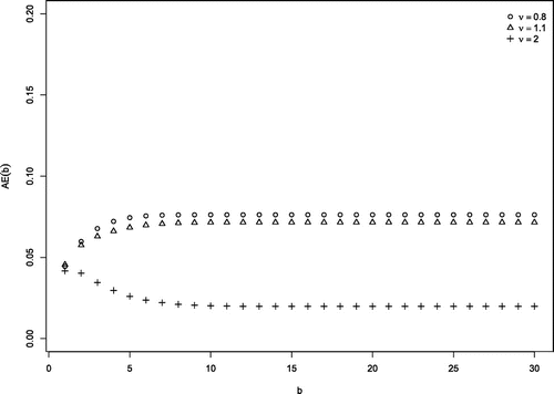
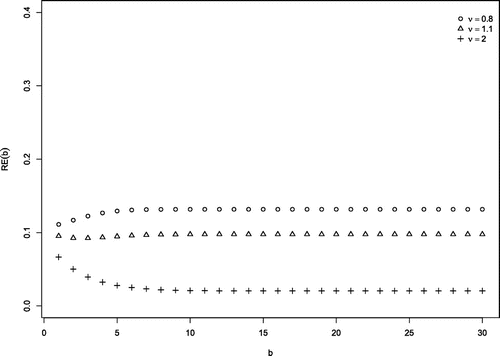
To assess the quality of these rough approximations we have investigated several scenarios and provide numerical outputs of the absolute and relative errors below in Figures 3–8. Two preliminary facts are immediate: Under scaling of all rates with the same factor $a\in (0,\infty ):\lambda \to a·\lambda ,$ etc. concurrently, the terms ${\beta }_b(f)$ are invariant, and therefore the relative error RE(b) is scale invariant, and the absolute error AE(b) scales linear in a (with a constant that is scale invariant).

In realistic scenarios the replenishment rate ν should guarantee that enough inventory is available to allow servicing of a reasonable portion of arrivals, that is, we assume ν is at least of the order of λ. Moreover, the individual perishing rate γ should be less than the arrival rate.

Exploiting the scale invariance of RE(b) and of the linear factor of AE(b), we henceforth fix λ = 1 and consider three scenarios with (1) fast perishing $\gamma =0.5$, (2) moderate perishing $\gamma =0.2$, and (3) slow perishing $\gamma =0.05$. In any scenario we consider replenishment rates $\nu =0.8/1.1/2$.

We have included “fast perishing” in order to show that our approach is not a panacea. We believe that this extreme case is not a realistic scenario.

From Figures 5–8 we see that in the moderate and slow perishing case the relative error is below 14%. Because the bounds for the approximation errors are very rough (“worst cases”), these maximal deviations of the product form bounds from the nonproduct form target value indicated by the experiments are astonishingly small.

7. Conclusion

For a large class of queueing-environment systems with bidirectional interaction, we have obtained product form steady state distributions. These explicit steady state distributions open the possibility to compute performance metrics of the systems explicitly.

If this direct access is not possible, we developed ergodicity and exponential ergodicity criteria using Lyapunov functions and demonstrated by an example of a coupled production-inventory system how to compute two-sided bounds for the throughput. This indicates how to proceed in cases of other queueing-environment systems to obtain explicit bounds for performance indices, which are not directly accessible. Another direction of research on nonseparable queueing-environment systems is to modify the transition rate matrix of the system suitably (possibly only the environment coordinate) to obtain a product form approximation of the stationary distribution. This is part of our ongoing research.

References

- (1991) Continuous-Time Markov Chains - An Application-Oriented Approach, vol. 7 of Springer Series in Statistics - Probability and its Applications (Springer, New York).Google Scholar
- (2003) Applied Probability and Queues, vol. 51 of Applications of Mathematics, 2nd ed. (Springer, New York).Google Scholar
- (1975) Open, closed and mixed networks of queues with different classes of customers. J. ACM. 22(2):248–260.Google Scholar
- (1999) Stochastic models for inventory management at service facilities. Commun. Stat. Stoch. Models. 15(4):695–718.Google Scholar
- (2000) Inventory management at service facilities for systems with arbitrarily distributed service times. Comm. Statist. Stoch. Models 16(3–4):343–360.Google Scholar
- (2002) Optimal service rates of a service facility with perishable inventory items. Naval Res. Logist. 49(5):464–482.Google Scholar
- (2011) On open problems in polling systems. Queueing Systems 68(3–4):365–374.Google Scholar
- (1967) Markov Chains with Stationary Transition Probabilities (Springer, Berlin).Google Scholar
- (1980) Markov chains in random environments: The case of Markovian environments. Ann. Probab. 8(5):908–916.Google Scholar
- (1984) The ergodic theory of Markov chains in random environments. Z. Wahrscheinlichkeitstheor. Verwandte Geb. 66(1):109–128.Google Scholar
- (1981) Birth and death processes with random environments in continuous time. J. Appl. Probab. 18(1):19–30.Google Scholar
- (1987) Birth and death processes in random environments with feedback. J. Appl. Probab. 24(1):25–34.Google Scholar
- (2016)
Moving queue on a network . Remke A, Haverkort BR, eds. Measurement, Modelling and Evaluation of Dependable Computer and Communication Systems, vol. 9629 of Lecture Notes in Computer Science (Springer, Cham, Switzerland), 40–54.Google Scholar - (2012) On a bilateral birth-death process with alternating rates. Ric. Mat. 61(1):157–169.Google Scholar
- (2014) Asymptotic results for random walks in continuous time with alternating rate. J. Statist. Phys. 154(5):1352–1364.Google Scholar
- (1990)
Single server queues with vacations . Takagi H, ed. Stochastic Analysis of Computer and Communication Systems (North–Holland, Amsterdam), 217–267.Google Scholar - (2003) A characterization of product-form stationary distributions for queueing systems in random environment. Proc. 17th Eur. Simulation Multiconf. (SCS-European Publishing House, Delft, Netherlands), 193–198.Google Scholar
- (2005) Generalized product-form stationary distributions for Markov chains in random environments with queueing applications. Adv. Appl. Probab. 37(1):185–211.Google Scholar
- (1996) A heterogeneous blocking system in a random environment. J. Appl. Probab. 33(1):211–216.Google Scholar
- (2012) Stability of a Markov-modulated Markov Chain, with application to a wireless network governed by two protocols. Stoch. Syst. 2(1):208–231.Link, Google Scholar
- (2016) A random walk in a queueing network environment. J. Appl. Probab. 53(2):448–462.Google Scholar
- (1984) Finite birth-and-death models in randomly changing environments. Adv. Appl. Probab. 16(4):715–731.Google Scholar
- (1984) Optimal control of arrivals to multiserver queues in a random environment. J. Appl. Probab. 21(3):602–615.Google Scholar
- (1957) Networks of waiting lines. Oper. Res. 5(4):518–521.Link, Google Scholar
- (2014) Perishable inventory system at service facilities with multiple server vacations and impatient customers. J. Statist. Appl. Probab. Lett. 3(3):63–73.Google Scholar
- (1976) Networks of queues. Adv. Appl. Probab. 8(2):416–432.Google Scholar
- (1979) Reversibility and Stochastic Networks (Wiley, Chichester, UK).Google Scholar
- (2014) Stochastic Networks. IMS Textbooks (Cambridge University Press, Cambridge, UK).Google Scholar
- (2017) Asymptotic analysis of the system with server vacation and perishable inventory. Cybernet. Systems Anal. 53(4):543–553.Google Scholar
- (2018) Models of perishable queueing-inventory systems with server vacation. Cybernet. Systems Anal. 54(1):31–44.Google Scholar
- (2016) Queueing systems in a random environment. PhD thesis, Universität Hamburg, Department of Mathematics, Hamburg, Germany.Google Scholar
- (2012) Loss Systems in a Random Environment—Steady State Analysis (Center of Mathematical Statistics and Stochastic Processes, Department of Mathematics, Hamburg University, Hamburg).Google Scholar
- (2014)
Modeling and performance analysis of a node in fault tolerant wireless sensor networks . Fischbach K, Krieger UR, eds. Measurement, Modelling, and Evaluation of Computing Systems and Dependability and Fault-Tolerance (Springer, Berlin), 73–87.Google Scholar - (2015a) Loss systems in a random environment - steady state analysis. Queueing Systems 80(1–2):127–153.Google Scholar
- (2015b)
Performability analysis of an unreliable M/M/1-type queue . Wolfinger BE, Heidtmann K-D, eds. Leistungs-, Zuverlässigkeits- und Verlässlichkeitsbewertung von Kommunikationsnetzen und verteilten Systemen, vol. 302. (Berichte des FB Informatik der Universität Hamburg, Hamburg, Germany), 90–95.Google Scholar - (2011) A survey on inventory models with positive service time. Opsearch 48(2):153–169.Google Scholar
- (2014) Queues with interruptions: A survey. TOP 22(1):290–320.Google Scholar
- (2019)
Inventory with positive service time: a survey . Anisimov V, Limnios N, eds. Advanced Trends in Queueing Theory: Series of Books “Mathematics and Statistics”, chapter 5 (ISTE & Wiley, London), 171–208.Google Scholar - (2007) A perishable inventory system with service facilities, MAP arrivals and PH-service times. J. Syst. Sci. Syst. Engrg. 16(1):62–73.Google Scholar
- (2008) A perishable inventory system with service facilities and retrial customers. Comput. Ind. Engrg. 54(3):484–501.Google Scholar
- (1992) Stock optimization in transportation/storage systems. Cybernet. Systems Anal. 28(3):484–487.Google Scholar
- (1981) Matrix Geometric Solutions in Stochastic Models - An Algorithmic Approach (Johns Hopkins University Press, Baltimore).Google Scholar
- (1979) Markovian queue with n servers subject to breakdowns and repairs. Management Sci. 25(9):849–861.Link, Google Scholar
- (1990) Numerical investigation of a multiserver retrial model. Queueing Systems 7(2):169–189.Google Scholar
- (2018) Integrated models for performance analysis and optimization of queueing-inventory-systems in logistic networks. PhD thesis, Universität Hamburg, Department of Mathematics, Hamburg, Germany.Google Scholar
- (2020) Stationary distributions and convergence for M/M/1 queues in interactive random environments. Queueing Systems 94(3–4):357–392.Google Scholar
- (1989) Markov-modulated queueing systems. Queueing Systems 5(1):215–245.Google Scholar
- (1995) Corrections to our paper: Markov-modulated queueing systems. Queueing Systems 19(4):449.Google Scholar
- (2013) The M/M/1 queue with inventory, lost sale, and general lead times. Queueing Systems 75(1):65–77.Google Scholar
- (2011) A queueing system with inventory and mixed exponentially distributed lead times. Internat. J. Adv. Manufacturing Tech. 53(9–12):1231–1237.Google Scholar
- (2003) Availability formulas and performance measures for separable degradable networks. Econom. Quality Control 18(2):165–194.Google Scholar
- (2006) M/M/1 Queueing systems with inventory. Queueing Systems 54(1):55–78.Google Scholar
- (1992) Light traffic heuristic for an M/G/1 queue with limited inventory. Ann. Oper. Res. 40(1):371–380.Google Scholar
- (1994) Strengthening ergodicity to geometric ergodicity for Markov chains. Comm. Statist. Stoch. Models 10(1):45–74.Google Scholar
- (2002)
Lectures on random motions in random media . Sznitman A-S, Bolthausen E, eds. Ten Lectures on Random Media, vol. 32 of DMV-Seminar (Birkhäuser Verlag, Basel), 9–51.Google Scholar - (1990)
Queueing analysis of polling models: An update . Takagi H, ed. Stochastic Analysis of Computer and Communications Systems (North-Holland, Amsterdam), 267–318.Google Scholar - (2008) Analysis of inventory systems with positive and negligible service time. PhD thesis, Department of Statistics, University of Calicut, Tenhipalam, India.Google Scholar
- (1989) Monotonicity of the throughput of a closed exponential queueing network in the number of jobs. OR Spectrum 11(6):97–100.Google Scholar
- (1993) Queueing Networks and Product Forms – A Systems Approach (Wiley, Chichester, UK).Google Scholar
- (1998) Bounds and error bounds for queueing networks. Ann. Oper. Res. 79(0):295–319.Google Scholar
- (2011)
On practical product form characterizations . Boucherie RJ, van Dijk NM, eds. Queueing Networks: A Fundamental Approach, vol. 154 of International Series in Operations Research and Management Science (Springer, New York), 1–83.Google Scholar - (1992) On product form approximations for communication networks with losses: error bounds. Ann. Oper. Res. 35(1):69–94.Google Scholar
- (1989) Simple bounds and monotonicity results for multi-server exponential tandem queues. Queueing Systems 4(1):1–16.Google Scholar
- (2015) A two heterogeneous servers perishable inventory system of a finite population with one unreliable server and repeated attempts. Pakistan J. Statist. 31(1):135–158.Google Scholar
- (2007) Stochastic inventory management at a service facility with a set of reorder levels. ORiON 28(2):137–149.Google Scholar
- (2012) A finite source multi-server inventory system with service facility. Comput. Ind. Engrg. 63(4):739–753.Google Scholar
- (1973) A queuing-type birth-and-death process defined on a continuous-time Markov chain. Oper. Res. 21(2):604–609.Link, Google Scholar
- (1994) Markovian queueing networks in a random environment. Oper. Res. Lett. 15(1):11–17.Google Scholar