On the Ergodic Properties and Invariant Measure of a Two-Dimensional Reflected Ornstein–Uhlenbeck Process
Abstract
We consider a two-dimensional reflected Ornstein–Uhlenbeck (ROU) process that arises as the diffusion approximation for a parallel server network with a randomly split Hawkes arrival process (or a multivariate Hawkes arrival process) in heavy traffic. We study the ergodic properties of the process, including the positive recurrence and rate of convergence in total variation distance and in Wasserstein distance. We also provide a numerical scheme based on a Monte Carlo method to approximate the invariant measure of the process.
Funding: G. Pang is partly supported by the National Science Foundation [Grants DMS 2216765 and CMMI 2452829].
1. Introduction
Reflected stochastic processes have attracted significant attention in recent years because of their close connections to queueing systems that arise in computer networks, telecommunications, mathematical biology, and transportation problems. Among the various areas of research, investigations into their ergodic properties have made striking progress. For instance, the recurrence of reflected Brownian motions and reflected diffusions has been widely explored in the literature, including, but not limited to, the references Williams (1985), Hobson and Rogers (1993), Dupuis and Williams (1994), Chen (1996), Budhiraja and Dupuis (1999), and Atar et al. (2001). Additionally, the stationary distributions of two-dimensional reflected Brownian motions have been thoroughly investigated, with explicit analytical expressions available. Relevant references include Harrison et al. (1985), Williams (1985), Dupuis and Ramanan (2002), Dieker and Moriarty (2009), Dai and Miyazawa (2011), and Franceschi and Raschel (2019). However, in higher dimensions, results on the stationary distribution are limited. Harrison and Williams (1987b) showed that under a certain skew symmetry condition, the stationary densities of reflected Brownian motions take an exponential product form. Despite this, Kang and Ramanan (2014) provided a characterization of stationary distributions of reflected diffusions.
However, when focusing specifically on the reflected Ornstein–Uhlenbeck process, the existing literature concentrates on the one-dimensional case. For example, Ward and Glynn (2003b) conducted a comprehensive study of the one-dimensional reflected Ornstein–Uhlenbeck (1-d ROU) process, including its explicit stationary density, a perturbation expansion for the transition density, and approximations for level crossing times. Furthermore, stationary distributions have been explored for certain generalized 1-d ROU processes. Specifically, Xing et al. (2009) investigated the 1-d ROU process with jumps and the 1-d Markov-modulated ROU process, whereas Zhang and Jiang (2009) studied the 1-d ROU process with two-sided barriers. Therefore, the main purpose of this paper is to extend the scope of research by studying a special case of the two-dimensional reflected Ornstein–Uhlenbeck process, as introduced below.
The two-dimensional reflected Ornstein–Uhlenbeck (2-d ROU) process in studied in this paper is defined as follows:
Before studying our 2-d process, we first provide an overview of the emergence of ROU processes. These processes arise as the diffusion scaling limit of a sequence of single-server queues with balking or reneging under heavy-traffic conditions (See Ward and Glynn 2003a, 2005 for details). Such queueing models have broad applications across various domains, including telecommunications, supply chain management, and computing and cloud services.
Beyond their derivation from such queueing models, ROU processes have also been shown to serve as effective approximations in various settings. Borovkov (1984) and Srikant and Whitt (1996) demonstrate that ROU processes approximate the number-in-system process in a G/M/s/0 queueing model when both the number of servers and the arrival rate are large. Additionally, Boxma et al. (2016) establish that the ROU process provides a heavy-traffic approximation for a sequence of reflected AR(1) processes.
However, these results focus primarily on the one-dimensional case. In contrast, our 2-d ROU process arises as the diffusion scaling limit for parallel single-server queues with abandonment in the critically loaded regime, which have a randomly split Hawkes process or a bivariate Hawkes process as the arrival processes (Li and Pang 2024). See Figure 1 for an illustration of these queueing models with split Hawkes arrivals. The correlation between these parallel queues emerges from dependencies in the arrival processes, which, in turn, translate into the correlated Brownian motions that drive the dynamics of the ROU process. Our 2-d ROU process is, of course, not the most general form of reflected OU processes; particularly, the drift is linear, the covariance coefficient is constant, and the reflection is normal. Furthermore, because there are no other interactions among the queues other than the arrivals, the reflection terms will be exactly like the reflection for each separate single-server queue with abandonment, as studied in Ward and Glynn (2005).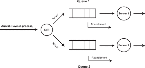
The analysis of our 2-d ROU process contributes to the understanding of stationary distributions and transient performance measures of these parallel server queueing models, where explicit expressions are often intractable. Furthermore, we believe our results may provide valuable insights into the stationary workload distribution of bivariate M/G/1 systems with coupled input and parallel service, as posed in Mandjes (2022).
For the one-dimensional ROU process, the ergodic properties are well understood, as discussed in Ward and Glynn (2003b), where the invariant measure is explicitly shown to have a truncated Gaussian distribution. Additionally, the exponential rate of convergence in total variation distance is studied in Lund et al. (1996), and the rate in Wasserstein distance is investigated in Sarantsev (2020). In this paper, our goal is to understand such ergodic properties for the simple 2-d ROU process arising from the parallel server queueing models mentioned above.
In pursuit of this goal, one potential method involves extending the methodologies used for 1-d ROU processes. However, this strategy appears to be intractable. Indeed, in both Ward and Glynn (2003b) and Xing et al. (2009), the study of the stationary distributions and the positive recurrence relies extensively on the explicit solutions to the corresponding ordinary differential equations (ODEs). When transitioning from the 1-d to the 2-d case, these ODEs transform into partial differential equations (PDEs), whose explicit solutions seem to be impossible to find. Moreover, their proofs use the result that the 1-d ROU processes are regenerative. However, in the two-dimensional case, this property appears no longer to hold, as 2-d processes are unlikely to revisit the same point infinitely often.
Furthermore, it might be tempting to consider the 2-d ROU process in (1.1) as a special case in the general class of constrained diffusion processes, which has been extensively studied in literature (Budhiraja and Dupuis 1999, Atar et al. 2001, Budhiraja et al. 2014, Kang and Ramanan 2014). However, these results cannot be directly applied to our 2-d ROU processes. For example, whereas the positive recurrence of constrained diffusions is well studied in Atar et al. (2001), their outcomes require strict constraints on the drift. As a result, they can only demonstrate the positive recurrence of our 2-d ROU processes when both and are (see Atar et al. 2001, condition 2.3). Nonetheless, a 2-d ROU process with positive does arise in practical applications. Specifically, if a sequence of parallel single-server queues has traffic intensities such that the limits of and exist and are positive; then, such a 2-d ROU process emerges as the diffusion scaling limit. Although this result was not explicitly stated in Li and Pang (2024), the derivation of the 2-d ROU process does not impose any constraints on these limits. On the other hand, it is important to explore the positive recurrence of 2-d ROU processes when . Indeed, when , the 2-d ROU process “dominates” the 2-d ROU process when , meaning and for all . Therefore, the positive recurrence of immediately implies that of . Hence, it is sufficient to prove the positive recurrence of with . A detailed explanation will be provided in Section 2. In this paper, we will establish the positive recurrence of the 2-d ROU process in all cases, thereby slightly extending the corresponding results in Atar et al. (2001) as applied to this process.
A common tool for studying the positive recurrence of reflected diffusion processes involves the use of the so-called “fluid path” or “fluid model,” which is a solution to the ODEs obtained by eliminating the randomness from the stochastic differential equations (SDEs) that define the reflected diffusion processes. It has been shown that the “fluid path” tending to the origin generally implies the recurrence of the reflected diffusion process. For more details, refer to Dupuis and Williams (1994), Atar et al. (2001), and Bramson et al. (2010). However, this tool is not applicable to our 2-d ROU processes when and are both positive. In fact, solving the following ODEs:
We first construct a discrete-time jump process from the original 2-d ROU process by restricting it to a sequence of elaborately selected stopping times such that one of and is zero for .
We then demonstrate that the above jump process reaches a given neighborhood of the origin within a finite mean time when starting from a position outside that neighborhood. Consequently, the original process exhibits the same property.
Finally, by focusing on the distance between and the origin and using the aforementioned property, we derive a similar regenerative process, enabling us to establish the positive recurrence.
It is worth mentioning that we believe our method, in conjunction with the Skorokhod maps for 1-d ROU processes, may be extended to address the case of oblique reflections. We have a strong inclination that 2-d ROU processes are always positive recurrent, irrespective of the reflection directions. We leave this question for future investigation.
The second contribution of this paper lies in studying the exponential rates of convergence to the stationary distribution. The existence and the uniqueness of the stationary distribution, which are the prerequisites for our study, have been previously explored in Kinnally and Williams (2010). Furthermore, our results shall provide an alternative proof of these properties. Following a similar argument as in (Khasminskii 2011, section 4.4), the existence can be established through the positive recurrence, whereas our subsequent results on convergence rates ensure the uniqueness.
Inspired by Lund et al. (1996) and Sarantsev (2020), we establish the convergence rates of the transition probability measures to the invariant measure in both total variation distance and Wasserstein distance. The derivation of the convergence rate in the total variation distance relies on the tail estimate of the first hitting time for the Ornstein–Uhlenbeck process (see Lemma 13), which affects the exponent involved in the convergence rate. On the other hand, for the Wasserstein distance, we establish a concise bound for the Wasserstein distance between two transition probability measures, resulting in an explicit exponent being , governing the rate of convergence to the invariant measure.
We next investigate the stationary distribution of the 2-d ROU process by a numerical scheme based on a Monte Carlo method. For diffusions, two common approaches for investigating the stationary distribution are the PDE method (refer to, e.g., Kurtz 1991, Dai and Kurtz 1994, Williams 1995) and the Monte Carlo method (see, e.g., Lamberton and Pages 2002, Talay 2002, Graham and Talay 2013). However, explicitly solving the PDEs derived from our process appears to be impossible. Therefore, we only focus on the Monte Carlo method. For reflected diffusions in polyhedral domains, Budhiraja et al. (2014) studied the numerical computation of their stationary distributions using an Euler scheme. However, their results cannot be directly applied to our case, as Budhiraja et al. (2014, conditions 1.3 and 1.4) are not satisfied. Therefore, utilizing the unique characteristics of our process, we develop our own numerical scheme for approximating the stationary distribution and also analyze the convergence of our scheme to the stationary distribution. This study is also in a similar spirit to the recent work in Jin et al. (2024a, b) on numerical methods using Euler–Maruyama schemes to compute the stationary distributions of limiting diffusions (without reflections) arising in approximations of queueing networks in heavy traffic. Similar to Budhiraja et al. (2014) and Jin et al. (2024a), our numerical scheme takes a decreasing step size.
Finally, it is worth mentioning that unlike the extensively studied ergodicity properties and stationary distributions of two-dimensional reflected Brownian motions (see, for instance, the recent work in El Kharroubp et al. 2000 and Franceschi and Raschel 2019), such studies on 2-d ROU processes seem to be lacking. Whereas the 2-d ROU processes investigated in this paper are not the most general, we contribute to this area by examining those properties for a specific case. In the future, we aim to extend our results to the most general ROU processes.
1.1. Overview of Our Contributions
Our contributions are as follows:
Prove the positive recurrence of the 2-d ROU process defined in (1.1); see Theorem 12.
Establish the exponential rates of convergence to its stationary distribution; see Theorems 15 and 17.
Provide a numerical scheme to approximate its stationary distribution; see Theorem 18.
1.2. Organization of the Paper
We first summarize the notation used in this paper at the end of this section. Section 2 is devoted to investigating the positive recurrence of the 2-d ROU process defined in (1.1), utilizing the aforementioned strategy. In Section 3, we examine the exponential rates of convergence to the stationary distribution in both total variation distance and Wasserstein distance. Finally, Section 4 focuses on analyzing a numerical scheme based on the Monte Carlo method to approximate the stationary distribution of the 2-d ROU process.
1.3. Notation
Let be the natural filtration space generated by the two-dimensional Brownian motion . Because are the solutions to the SDE (1.1), they are also processes on . Throughout the paper, denotes the two-dimensional positive orthant, and represents its boundary. Additionally, we use to denote the set . For , we use and to denote the probability and the expectation, respectively, when the 2-d ROU process starts from . Similarly, for a 1-d process starting from , and are the corresponding probability and expectation. Moreover, for , we define , , and . Additionally, is the Dirac measure on concentrated at . For a set A, we use to represent the indicator function of A.
When studying the convergence rates to the stationary distribution, we will need the following notation. We denote the stationary distribution as . Furthermore, for , represents the transition probability measure for the 2-d ROU process. Finally, we introduce total variation distance and Wasserstein distance. Given two measures and on , the total variation distance is defined by
Additional notation is introduced in the paper as needed.
2. Positive Recurrence
The aim of this section is to study the positive recurrence of the 2-d ROU process defined in (1.1), following the strategy outlined in Section 1.
2.1. Preliminary
We start by citing a lemma from Ward and Glynn (2003b), which demonstrates that a 1-d ROU process is “controlled” or “dominated” by a 1-d reflected Brownian motion (RBM) with the same parameters. This lemma allows us to exploit the properties of the 1-d RBM to study the ROU process. Subsequently, we extend this lemma to compare between two 1-d ROU processes, and the result is summarized in Lemma 2.
Let X be a 1-d ROU process satisfying
See Ward and Glynn (2003b, proof of roposition 2). □
Let X be a 1-d ROU process satisfying
Suppose that there exists for which . By assumptions, . Furthermore, noting that has continuous sample paths, there exists such that , but for . Hence, for . Note that
Because is nondecreasing, it follows
Noting that for and is a continuous process that increases only when X equals zero, we conclude . Therefore, , which is a contradiction. □
By using a similar argument, the result in Lemma 2 still holds if the 1-d ROU processes are replaces by two 1-d Ornstein–Uhlenbeck processes. Furthermore, we can also prove a 1-d Ornstein–Uhlenbeck process is bounded above by a 1-d ROU process with the same parameters.
With the above lemma in hand, we are ready to show that it is sufficient to prove the positive recurrence when both and are nonnegative, as promised in Section 1. Indeed, if at least one of and is negative, we can construct a new 2-d ROU process by the following SDEs:
With the above preparation, we now return to the proof of the positive recurrence. For any neighborhood of the origin, we define
In what follows, we will prove that for any . Consequently, the positive recurrence follows. Here, the symbol represents the expectation when the 2-d ROU process starts from . The proof will be divided into three subsections, aligning with the three steps described in Section 1.
2.2. Stopping Times
In this subsection, we will first introduce certain stopping times and estimate their expectations. These will serve as the basis for defining a sequence of stopping times, enabling us to construct the jump process. Moreover, we will provide estimates for the expectation of , as well as the position of at .
Define
Indeed, and are the first hitting times of X and Y to zero, respectively. If X starts at zero, we define
Thus, is the first time that X returns to zero after it hits one. Additionally, can also be written as
Here, is a shift operator, the effect of which on a path is to cut off the part of the path before and to shift the remaining part in time. Similarly, if Y starts at zero, we define
Again, is the first time that Y returns to zero after it hits one, and can be written as
Once these stopping times are defined, we can proceed to provide estimates for their expectations, which are summarized in Lemma 4, Lemma 5, and Lemma 6.
For any , we have
Furthermore,
The first statement is an immediate consequence of Ward and Glynn (2003b, proposition 4). We then turn to the second statement. By the symmetry, we only need to derive (2.3) from (2.1).
By substituting the variable , we have
If ,
If , using the upper bound for the tail of the standard normal distribution,
When , combining the above two displays together with (2.1), we have
When , it is immediate that . Combining these two cases, (2.3) follows. □
For any , we have
Thus, we use constants and to denote and , respectively.
See Ward and Glynn (2003b, theorem 2). □
With the above two lemmas and the fact that and , we are ready to establish Lemma 6.
For any , we have
We only prove (2.5), and (2.6) follows similarly.
By the strong Markov property,
By Lemma 5, we have
By Lemma 4, we have
The desired result follows by combining the above three displays. □
The three lemmas above provide bounds for the expectations of the stopping times. To define and analyze the jump process mentioned in Section 1, we also need to evaluate the position of at a given stopping time. The following lemma, which provides a bound for the expectation of a one-dimensional Ornstein–Uhlenbeck process at any stopping time, will be a valuable tool for this purpose.
Let Z be a one-dimensional Ornstein–Uhlenbeck process satisfying
It is immediate that Z has the expression
By substituting R for t and applying the triangle inequality, it easily follows that
We then evaluate the expectation of . By Itô’s lemma,
Using the optional sampling theorem yields
Letting , together with Fatou’s lemma and monotone convergence theorem, we have
It follows by Jensen’s inequality that
By taking expectation on both sides of (2.7) and combining it with the above display, the desired result follows. □
Next, we introduce a new stopping time, S, related to , and . This stopping time is a key ingredient in defining the jump process and is defined as follows:
If starts at , then .
If starts at , then .
In other words, if the process starts from a point on , the stopping time S means the first time when either one component of the pair reaches zero or the other that starts at zero reaches one and then returns to zero. In particular, if the process starts from , both two definitions result in .
Before introducing the sequence of stopping times that defines the jump process, we pause to examine the properties of S. Indeed, we will estimate the expectations of S and , as summarized in Lemma 8 and Lemma 9, respectively.
We begin with Lemma 8.
For any , we always have
If starts at , it follows by Lemma 6 and the definition of S that
Similarly, if starts at , we have . The desired result follows by combining the above two cases. □
The following lemma concerns the expectation of .
For any , we have
We only prove (2.8), and (2.9) follows similarly.
By the definition of S, when starts at ,
Applying Lemma 7 yields
Similarly, when starts at , noting that , we have
Because for , we have ; thus,
Taking expectation yields
Applying Lemma 7 yields
Combining the last display with (2.10), the desired result follows. □
With Lemma 9 in hand, We immediately obtain Corollary 10 as follows:
There are constants , and such that for any ,
Consequently, there exist sufficiently large B and such that if and , then
In the rest of the section, we will use to denote the set .
With the above preparation, we are ready to introduce the stopping times and the jump process as mentioned in Section 1.
Define , , and
By the strong Markov property and Lemma 8, we have, for ,
Additionally, we define the jump process as follows:
2.3. Reachability of the Jump Process to the Neighborhood of the Origin
In this subsection, we will prove that if the process starts from a point on , then it will eventually reach within a finite mean time. Consequently, the same property holds for the original 2-d ROU process.
The preceding statements are summarized in the following lemma.
Define . We have almost surely. Furthermore,
Therefore, the 2-d ROU process , starting from a point on , will eventually reach the region within an expected time of at most .
We claim is a nonnegative supermartingale with respect to the filtration . Recall that is the natural filtration generated by . Therefore, represents the corresponding -field stopped at . It is immediate that and are -measurable because and .
We now turn to verify the above claim.
Given that , it follows by letting that almost surely. Therefore, the jump process inevitably hits the region . If we look back at the 2-d ROU process , we can conclude that must hit if it starts from a point on .
Note that the first time when hits is less than or equal to . In the next step, we estimate the expectation of and, consequently, the expected time for the process to visit . Indeed, by Lemma 8 and the strong Markov property,
Therefore, for the 2-d ROU process starting from a point on , it eventually reaches the region with an expected time no greater than . □
2.4. Positive Recurrence
The purpose of this subsection is to provide the main (theorem Theorem 12) of this section, which focuses on the positive recurrence of the 2-d ROU process .
Recall T is the first time the process hits the neighborhood of the origin.
There exists a constant (see (2.19)) such that for any
Define
H is the first time that the process hits the area . We first prove
Note that ; thus, by Lemma 4,
To bound , it remains to provide an upper bound for , which depends on the estimate for . To achieve this, we note that for , behaves like a 2-d Ornstein–Uhlenbeck process. Using a similar argument as in the proof of Lemma 9, we conclude
Then, by the strong Markov property,
We have already proven that the process , starting from any point on , will reach within a time H whose mean is bounded by (up to a constant). We then define
To finish the proof, we need the following result:
There is a constant such that
The proof of this result relies on the standard properties of Brownian motion. By Lemma 1, we can construct a 2-d reflected Brownian motion such that and for any . Define and for similarly to T and R, respectively. By a standard property of Brownian motion, there exists such that for all , (refer to Hobson and Rogers 1993). Thus,
We now return to complete the proof. We define
It follows immediately from the definition of H and R that and for . Considering the Estimate (2.14) and applying the strong Markov property, we have, for ,
Thus, noting that , we obtain, for ,
From the above estimate, we conclude that for ,
Then, is a stopping time with respect to the filtration because . Applying the optional sampling theorem yields
Letting and applying the monotone convergence theorem, we have
Together with (2.14), we have
It follows immediately from the definition of M that ; thus,
What remains is to estimate the expectation of M.
For any , by the strong Markov property,
Continuing the above procedure recursively, we have
Because ,
Plugging the above result into (2.18) gives
We conclude the proof. □
3. Exponential Rate of Convergence
The section aims to investigate the rate of convergence to the stationary distribution of the 2-d ROU process. We will provide exponential rates of convergence in both total variation distance and Wasserstein distance. Further, we will explicitly specify the exponent for the latter.
3.1. A Tail Estimate for the First Hitting Time of an OU Process
Before addressing the rate of convergence, we first present a (lemma Lemma 13) regarding the tail estimate of the first hitting time for an Ornstein–Uhlenbeck process, which is the main ingredient in studying the rate of convergence in total variation distance.
Let Z be a one-dimensional Ornstein–Uhlenbeck process driven by the SDE
Then, for any , there exist constants and depending on , and such that for ,
We start by considering the case where . Our approach to estimating will be divided into three cases based on the value of z: (i) , (ii) , and (iii) .
. Using Alili et al. (2005, corollary 3.2) (after an appropriate transformation), we have that for any , there exist constants and depending on , and such that for ,
. By applying Remark 3, Z is bounded above by the Ornstein–Uhlenbeck process with the same parameters, but starting at ; hence, for ,
. We define
Thus, in the event , we have . Let be a Brownian motion with a drift driven by the SDE:
By a similar argument to that in the proof of Lemma 1, we have for . Thus, . Then, we have
Then, together with the strong Markov property, we have, for ,
Combining the above three cases gives, for and ,
What remains is the case that . Indeed, the desired result follows from the fact that is bounded by the Ornstein–Uhlenbeck process with . We conclude the proof. □
3.2. Exponential Rate of Convergence in Total Variation Distance
This subsection is devoted to the rate of convergence in total variation distance. It begins by studying the total variation distance between two transition probability measures, followed by the total variation distance between the transition probability measure and the invariant measure.
Recall that is the transition probability measure for the process when it starts from , and represents the stationary distribution.
Fix . For any , there exist constants , depending on , and , and , , depending on , and such that for ,
For , we use to denote the 2-d ROU process satisfying the SDEs
Further, we define
We first claim that on the event , . This will be demonstrated subsequently. Without loss of generality, we assume that . Applying Lemma 2, we have for . Thus, , and . Because is nonnegative, then
Similarly, in the event , we have .
With the above preparation, we proceed to study the total variation distance between and . It follows from the definition of total variation distance that
Note that in the event , . Thus,
Taking expectation on both sides of the last display and then taking supremum over A from , we have
What remains is to evaluate and . Without loss of generality, we assume ; then, and
On the event , behaves like an Ornstein–Uhlenbeck process; hence, is the first hitting time to zero for an Ornstein–Uhlenbeck process. By Lemma 13, for any , there are constants and depending on , and such that for ,
Together with (3.2), we have
Similarly, there exist constants and depending on , and such that for ,
The desired result follows by combining (3.1), (3.3), and (3.4). □
With Theorem 14 in hand, we are ready to study the rate of convergence to the stationary distribution in total variation distance.
Fix . For any , there exist constants , depending on , and y, and , depending on , and , such that for ,
It can be easily verified that
Plugging the result of Theorem 14 into the above display, after arrangement, we have, for ,
Note that the marginal measures of are stationary distributions for 1-d ROU processes; hence, they have truncated Gaussian distributions (cf. Ward and Glynn 2003b, proposition 1). Consequently,
Then, the desired result follows. □
3.3. Exponential Rate of Convergence in Wasserstein Distance
This subsection aims to demonstrate that the rate of convergence in Wasserstein distance is exponential, with the exponent being explicit. Again, we begin by examining the Wasserstein distance between two transition probability measures and then turn to the Wasserstein distance between any transition probability measure and the stationary distribution.
For , we have, for ,
We adopt the notation in the proof of Theorem 14. That is, is the 2-d ROU process starting from , and and are the first hitting times to zero.
By the definition of Wasserstein distance,
Note that f is a Lipschitz function with Lipschitz constant . Thus,
Taking expectation on both sides of the last display and then taking supremum over f from , we have
In what follows, we will evaluate the expectations of and . We begin with the expectation of . Without loss of generality, we assume that . Let be an Ornstein–Uhlenbeck process satisfying the SDE
Using Lemma 2 and Remark 3, we have, for ,
By a similar argument in the proof of Theorem 14, we conclude on the event . Thus, combining these two results yields
In the event , behaves like an Ornstein–Uhlenbeck process and, hence, has the representation
Then, plugging (3.6) and (3.8) into (3.7) gives
Thus,
Similarly,
Combining (3.5), (3.9), and (3.10), the desired result follows. □
For , there exist constants , depending on , and x, and , depending on , and y, such that for ,
It can be easily verified that
Together with Theorem 16, we have
Because the marginal measure has a truncated Gaussian distribution,
4. A Numerical Scheme for the Stationary Distribution
The purpose of this section is to numerically study the stationary distribution for the 2-d ROU process. For diffusions, two common approaches for investigating the stationary distribution are the PDE method and the Monte Carlo method. We begin by presenting the PDE that the density of the stationary distribution satisfies, along with the corresponding boundary conditions, provided the existence of the density. However, because of its complexity, we are unable to solve this PDE ourselves and defer it to the experts in PDE. Therefore, we turn to the Monte Carlo method, which is partly inspired by Budhiraja et al. (2014). Additionally, the Monte Carlo method has an advantage in higher dimensions. Indeed, the approach we will elaborate on later can be automatically extended to high-dimensional ROU processes.
4.1. Stationary Distribution: A PDE Perspective
Assume the stationary distribution, denoted , is absolutely continuous with density function . Indeed, we believe the assumption can be justified by modifying the argument in Harrison and Williams (1987a, section 7). However, as this is beyond the scope of the paper, we omit the detailed verification. In the following, we will characterize by introducing the corresponding PDE.
For any smooth function f on with compact support on , an application of Itô’s lemma gives
Noting that , are bounded and , it follows by taking expectation that
Because is the stationary distribution for , we have . Then,
Hence,
Because we assume is the density function of , we have
Using integration by parts yields
Here, can be understood as weak derivatives. By the arbitrariness of f, we conclude
We now turn to the boundary conditions for . Because and are one-dimensional reflected Ornstein–Uhlenbeck processes, the marginal distributions of correspond to the stationary distributions of and ; that is,
In summary, satisfies the following PDE:
We are unable to solve the above PDE, as its boundary conditions do not fall into standard categories such as Dirichlet, Neumann, or Robin. So we entrust the task to experts in PDE.
4.2. Numerical Scheme and Its Convergence
In this subsection, we will develop a convergent numerical procedure to approximate the stationary distribution of our ROU process. Consistently, the stationary distribution is denoted by . We begin by constructing a discrete-time process that serves as an approximation to the ROU process.
Let be a sequence of real numbers satisfying the following conditions:
for all ;
as ;
as .
Here, is the set of all positive integers. Note that the above conditions are satisfied if with . Let be a sequence of independent and identically distributed (i.i.d.) random vectors in with mean and covariance matrix . Furthermore, we pose the following assumption on ’s:
With the above preparation, we are ready to iteratively construct a discrete-time process in . For , define
With these random measures in hand, we are now prepared to introduce the main result of this section.
As , converges weakly to almost surely.
The proof of Theorem 18 is relegated to the following two subsections.
4.3. Tightness
The aim of this subsection is to establish the tightness of almost surely. To this end, we prepare the following lemmas.
For nonnegative integers n, l, we have
We only prove (4.2), and (4.3) follows similarly.
Define
Then,
Dividing by on both sides yields
In the last display, by letting , and summing up these l equations, we have
For simplicity of notation, we define
Thus,
At this stage, we fix n and allow l to vary. Then, is nonnegative for all . , viewed as a function of l, is nondecreasing. Furthermore, increases at l only if , which occurs only if according to the definition of . Combining the above observations, together with the uniqueness of the Skorokhod map, it follows that
Thus,
Note that for ,
Combining the last three displays, together with the nonnegativity of , we have
To prove (4.2), it remains to prove
Indeed, noting that for , it follows that
Comparing (4.3) and (4.6) and repeating this procedure, we have
Combining the last two displays yields (4.4). We conclude the proof. □
For nonnegative integers n, l, and any , we have
Consequently, it follows by Hölder’s inequality that
By symmetry, we only prove (4.7).
Note that
For fixed n and l, because are independent with a zero mean,
With these two lemmas in hand, we can establish a uniform upper bound for the expectations of . This result is summarized in the following lemma.
For any , we have
Letting in Lemma 19 and noting that yield
Similarly,
Combining the last two displays with Lemma 20, the desired result follows. □
Before presenting the next result, we introduce some necessary notation. Define and as
For any , it can be easily verified that
For any , define
Then, for any , we have
Applying Lemma 19 and Lemma 20, together with the independence of the sequence , we have
In fact, if and , then and . Therefore,
Note that . It follows that
Similarly,
Combining the last two displays with (4.8), we have
We conclude the proof. □
With the above preparation, we arrive at our primary result in this subsection, indicating the almost sure tightness of the sequence of random measures .
For any , we have
The proof is similar to that of Budhiraja et al. (2014, lemma 6); therefore, we omit the specific details. □
4.4. Identification of the Limit
To complete the proof of Theorem 18, we must demonstrate that for almost every , any weak limit of is . To this end, we follow the method in Budhiraja et al. (2014, section 2.2). It is worth noting that all the conditions necessary for the deduction in Budhiraja et al. (2014, section 2.2) are satisfied, except for the requirement of boundedness in , which corresponds to the boundedness of and in our case. However, and . When modifying the proof in Budhiraja et al. (2014, section 2.2), it only requires the following results:
(R1) almost surely as ;
(R2) For any nonnegative integer j,
almost surely as ;(R3)
All the results can be derived from Lemma 21 and Proposition 23. Indeed, note that
Therefore, (R1) follows immediately from Proposition 23 and the fact that and . Furthermore, (R2) follows similarly because
Finally, (R3) follows from the uniform boundedness of , which is a direct result of Lemma 21. This completes the convergence analysis of the numerical scheme.
4.5. Numerical Results
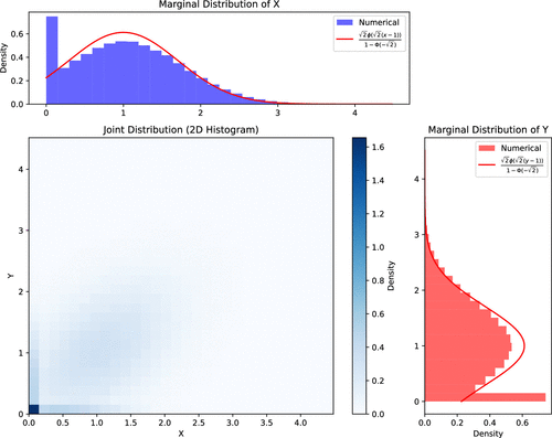
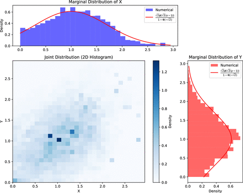
In this subsection, we apply our numerical scheme to approximate the stationary distribution of the 2-d ROU process under the parameter setting , , with initial conditions and . The resulting numerical joint and marginal distributions are computed using three different schemes: (i) , (ii) , and (iii) . The number of iterations is set to . Additionally, the true marginal distributions, with density functions given by and , are plotted as red curves to enable comparison and evaluate the accuracy of the numerical approximations.
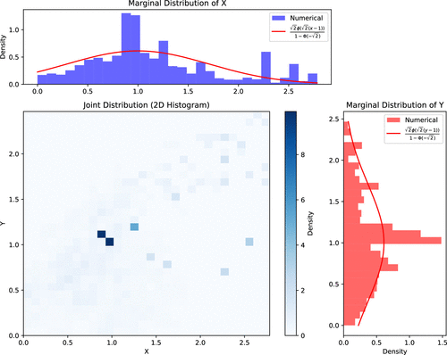
The selection of the step size presents a challenge. When the number of iterations is relatively small, the step size should be chosen carefully to balance accuracy and stability. If the step size is too large, such as , the discretized process , as defined in Section 4.2, may frequently visit , resulting in an approximating distribution that is overly concentrated at . Moreover, as illustrated in Figure 2, the marginal distributions exhibit a good fit except at zero. Conversely, if the step size is too small, for instance, , the discretized process tends to remain near the initial position , leading to an approximating distribution concentrated at and thus producing an inaccurate result (see Figure 4). In contrast, when the step size is moderate, the approximating distribution is more dispersed. As suggested by the marginal distribution diagrams in Figure 3, we believe this choice provides a closer approximation to the true stationary distribution.
We proceed to numerically estimate the correlation of the 2-d ROU processes under different parameter settings, using the scheme . Specifically, we use the empirical correlation
|

Table 1. Numerical Results for the Correlation of the 2-d ROU Process for Different Values of When , , , , and
| 0.1 | 0.2 | 0.3 | 0.4 | 0.5 | 0.6 | 0.7 | 0.8 | 0.9 | |
|---|---|---|---|---|---|---|---|---|---|
| 0.0418 | 0.2164 | 0.1753 | 0.3079 | 0.5332 | 0.5777 | 0.6734 | 0.7603 | 0.8900 | |
| −0.1 | −0.2 | −0.3 | −0.4 | −0.5 | −0.6 | −0.7 | −0.8 | −0.9 | |
| −0.0023 | −0.1475 | −0.2464 | −0.4193 | −0.4744 | −0.5402 | −0.6105 | −0.7403 | −0.8265 |
|
Table 2. Numerical Results for the Correlation of the 2-d ROU Process for Different Values of When , , , , and
| 0.1 | 0.2 | 0.3 | 0.4 | 0.5 | 0.6 | 0.7 | 0.8 | 0.9 | |
|---|---|---|---|---|---|---|---|---|---|
| 0.1245 | 0.1321 | 0.2275 | 0.3704 | 0.4188 | 0.5192 | 0.5969 | 0.7785 | 0.8696 | |
| −0.1 | −0.2 | −0.3 | −0.4 | −0.5 | −0.6 | −0.7 | −0.8 | −0.9 | |
| −0.0650 | −0.0819 | −0.0689 | −0.2009 | −0.2321 | −0.2138 | −0.3121 | −0.3374 | −0.4103 |
|
Table 3. Numerical Results for the Correlation of the 2-d ROU Process for Different Values of When , , , , , , and
| 0.1 | 0.2 | 0.3 | 0.4 | 0.5 | 0.6 | 0.7 | 0.8 | 0.9 | |
|---|---|---|---|---|---|---|---|---|---|
| 0.0642 | 0.1475 | 0.1543 | 0.2531 | 0.3766 | 0.4446 | 0.4741 | 0.6062 | 0.6823 | |
| −0.1 | −0.2 | −0.3 | −0.4 | −0.5 | −0.6 | −0.7 | −0.8 | −0.9 | |
| −0.0586 | −0.1079 | −0.1896 | −0.3056 | −0.3685 | −0.3285 | −0.4681 | −0.5157 | −0.5567 |
|
Table 4. Numerical Results for the Correlation of the 2-d ROU Process for Different Values of ρ When , , , , , and
| 0.1 | 0.2 | 0.3 | 0.4 | 0.5 | 0.6 | 0.7 | 0.8 | 0.9 | |
|---|---|---|---|---|---|---|---|---|---|
| 0.0975 | 0.1036 | 0.1952 | 0.3467 | 0.3913 | 0.4959 | 0.5873 | 0.7614 | 0.8504 | |
| −0.1 | −0.2 | −0.3 | −0.4 | −0.5 | −0.6 | −0.7 | −0.8 | −0.9 | |
| −0.0909 | −0.1098 | −0.0943 | −0.2434 | −0.2672 | −0.2525 | −0.3485 | −0.3766 | −0.4726 |
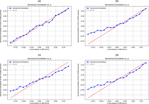
Notes. (a) Corresponding to Table 1. (b) Corresponding to Table 2. (c) Corresponding to Table 3. (d) Corresponding to Table 4.
We close this subsection by approximating the Laplace transform of the stationary distribution , namely, , employing the empirical Laplace transform
We adopt the parameter setting: , , , , , with initial conditions and . We employ the scheme and set the number of iterations to . For the parameters s and t, we consider the values and compute the corresponding results, which are summarized in Table 5.
|
Table 5. Numerical Results for the Laplace Transform When , , , , , , and
| s\t | 0.1 | 0.5 | 1.0 | 2.0 | 10.0 |
|---|---|---|---|---|---|
| 0.1 | 0.924452 | 0.776782 | 0.649057 | 0.494020 | 0.211610 |
| 0.5 | 0.828981 | 0.701933 | 0.591122 | 0.455137 | 0.200988 |
| 1.0 | 0.734828 | 0.627416 | 0.532873 | 0.415452 | 0.189715 |
| 2.0 | 0.601916 | 0.520769 | 0.448313 | 0.356592 | 0.172038 |
| 10.0 | 0.285189 | 0.256977 | 0.230848 | 0.196018 | 0.115423 |
The authors thank the reviewers for their helpful comments that have led to great improvement in the exposition of the results. The authors also express their sincere gratitude to Dr. Sumith Reddy Anugu for his invaluable contributions to this research.
References
- (2005) Representations of the first hitting time density of an Ornstein–Uhlenbeck process. Stochastic Models 21(4):967–980.Google Scholar
- (2001) On positive recurrence of constrained diffusion processes. Ann. Probab. 29(2):979–1000.Google Scholar
- (1984) Asymptotic Methods in Queuing Theory (John Wiley & Sons, New York).Google Scholar
- (2016) On a class of reflected AR (1) processes. J. Appl. Probab. 53(3):818–832.Google Scholar
- (2010) Positive recurrence of reflecting Brownian motion in three dimensions. Ann. Appl. Probab. 20(2):753–783.Google Scholar
- (1999) Simple necessary and sufficient conditions for the stability of constrained processes. SIAM J. Appl. Math. 59(5):1686–1700.Google Scholar
- (2014) A numerical scheme for invariant distributions of constrained diffusions. Math. Oper. Res. 39(2):262–289.Link, Google Scholar
- (1996) A sufficient condition for the positive recurrence of a semimartingale reflecting Brownian motion in an orthant. Ann. Appl. Probab. 6(3):758–765.Google Scholar
- (1994) Characterization of the stationary distribution for a semimartingale reflecting Brownian motion in a convex polyhedron. Preprint 1–31.Google Scholar
- (2011) Reflecting Brownian motion in two dimensions: Exact asymptotics for the stationary distribution. Stochastic Systems 1(1):146–208.Link, Google Scholar
- (2009) Reflected Brownian motion in a wedge: Sum-of-exponential stationary densities. Electronic Comm. Probab. 14:1–16.Google Scholar
- (2002) A time-reversed representation for the tail probabilities of stationary reflected Brownian motion. Stochastic Processes Appl. 98(2):253–287.Google Scholar
- (1994) Lyapunov functions for semimartingale reflecting Brownian motions. Ann. Probab. 22(2):680–702.Google Scholar
- (2000) Sur la récurrence positivedu mouvement brownien réflechidans l’orthant positif de . Stochastics Stochastic Rep. 68(3–4):229–253.Google Scholar
- (2021) Escape and absorption probabilities for obliquely reflected Brownian motion in a quadrant. Stochastic Processes Appl. 142:634–670.Google Scholar
- (2019) Integral expression for the stationary distribution of reflected Brownian motion in a wedge. Bernoulli 25(4B):3673–3713.Google Scholar
- (2013) Stochastic Simulation and Monte Carlo Methods: Mathematical Foundations of Stochastic Simulation, Stochastic Modelling and Applied Probability, vol. 68 (Springer, Berlin, Heidelberg).Google Scholar
- (1987a) Brownian models of open queueing networks with homogeneous customer populations. Stochastics 22(2):77–115.Google Scholar
- (1987b) Multidimensional reflected Brownian motions having exponential stationary distributions. Ann. Probab. 15(1):115–137.Google Scholar
- (1985) The stationary distribution of reflected Brownian motion in a planar region. Ann. Probab. 13(3):744–757.Google Scholar
- (1993) Recurrence and transience of reflecting Brownian motion in the quadrant. Math. Proc. Cambridge Philos. Soc. 113(2):387–399.Google Scholar
- (2024a) Approximation of the steady state for piecewise stable Ornstein-Uhlenbeck processes arising in queueing networks. Preprint, submitted May 29, https://arxiv.org/html/2405.18851v1.Google Scholar
- (2024b) An approximation to the invariant measure of the limiting diffusion of G/Ph/n+ GI queues in the Halfin–Whitt regime and related asymptotics. Math. Oper. Res. 50(2):783–812.Google Scholar
- (2014) Characterization of stationary distributions of reflected diffusions. Ann. Appl. Probab. 24(4):1329–1374.Google Scholar
- (2011) Stochastic Stability of Differential Equations, Stochastic Modelling and Applied Probability, vol. 66 (Springer, Berlin, Heidelberg).Google Scholar
- (2010) On existence and uniqueness of stationary distributions for stochastic delay differential equations with positivity constraints. Electronic J. Probab. 15:409–451.Google Scholar
- (1991)
A control formulation for constrained Markov processes . Kohler WE, White BS, eds. Mathematics of Random Media, Lectures in Applied Mathematics, vol. 27 (American Mathematical Society, Providence, RI).Google Scholar - (2002) Recursive computation of the invariant distribution of a diffusion. Bernoulli 8(3):367–405.Google Scholar
- (2016) Brownian Motion, Martingales, and Stochastic Calculus, Graduate Texts in Mathematics, vol. 274 (Springer, Cham, Switzerland).Google Scholar
- (2024) Heavy-traffic limits for parallel single-server queues with randomly split Hawkes arrival processes. J. Appl. Probab. 61(2):490–514.Google Scholar
- (1984) Stochastic differential equations with reflecting boundary conditions. Comm. Pure Appl. Math. 37(4):511–537.Google Scholar
- (1996) Computable exponential convergence rates for stochastically ordered Markov processes. Ann. Appl. Probab. 6(1):218–237.Google Scholar
- (2022) Multivariate m/G/1 systems with coupled input and parallel service. Queueing Systems 100(3):309–311.Google Scholar
- (2020) Convergence rate to equilibrium in Wasserstein distance for reflected jump–diffusions. Statist. Probab. Lett. 165:108860.Google Scholar
- (1996) Simulation run lengths to estimate blocking probabilities. ACM Trans. Modeling Comput. Simulation 6(1):7–52.Google Scholar
- (2002) Stochastic Hamiltonian systems: Exponential convergence to the invariant measure, and discretization by the implicit Euler scheme. Markov Processes Related Fields 8(2):163–198.Google Scholar
- (2003a) A diffusion approximation for a Markovian queue with reneging. Queueing Systems 43:103–128.Google Scholar
- (2003b) Properties of the reflected Ornstein–Uhlenbeck process. Queueing Syst. 44(2):109–123.Google Scholar
- (2005) A diffusion approximation for a GI/GI/1 queue with balking or reneging. Queueing Systems 50:371–400.Google Scholar
- (1985) Recurrence classification and invariant measure for reflected Brownian motion in a wedge. Ann. Probab. 13(3):758–778.Google Scholar
- (1995)
Semimartingale reflecting Brownian motions in the orthant . Kelly FP, Williams RJ, eds. Stochastic Networks, The IMA Volumes in Mathematics and Its Applications, vol. 71 (Springer, New York), 125–137.Google Scholar - (2009) The stationary distributions of two classes of reflected Ornstein–Uhlenbeck processes. J. Appl. Probab. 46(3):709–720.Google Scholar
- (2009) Stationary distribution of reflected O–U process with two-sided barriers. Statist. Probab. Lett. 79(2):177–181.Google Scholar