State Spaces of Multifactor Approximations of Nonnegative Volterra Processes
Abstract
We show that the state spaces of multifactor Markovian processes, coming from approximations of nonnegative Volterra processes, are given by explicit linear transformations of the nonnegative orthant. We demonstrate the usefulness of this result for applications, including simulation schemes and partial differential equation methods for nonnegative Volterra processes.
Funding: E. Abi Jaber gratefully acknowledges financial support from the Chaires Laboratoire de Finance des Marchés de l’Énergie-Finance et Développement Durable and Financial Risks at École Polytechnique. C. Bayer and S. Breneis gratefully acknowledge the support by the International Research Training Group 2544 “Stochastic Analysis in Interaction.” C. Bayer also acknowledges support from Deutsche Forschungsgemeinschaft Collaborative Research Center/Transregio 388 “Rough Analysis, Stochastic Dynamics and Related Fields” [Project B02].
1. Introduction
Multifactor Markovian approximations for fractional Brownian motion were initially introduced by Carmona and Coutin (1998) and revisited more recently by Abi Jaber and El Euch (2019b) in the context of nonnegative stochastic Volterra equations, motivated by rough and Volterra Heston models of El Euch and Rosenbaum (2019) and Abi Jaber et al. (2019b). Since then, substantial literature has emerged on such multifactor processes for numerical approximation methods (Harms 2019; Chevalier et al. 2022; Bayer and Breneis 2023a, b, 2024; Alfonsi and Kebaier 2024), deep learning approaches (Papapantoleon and Rou 2025), modeling (Abi Jaber 2019), and optimal control (Abi Jaber et al. 2021). It should be noted that such approximations are also heavily used in physics, chemistry, and other fields; see, for example, Baczewski and Bond (2013) and Bochud and Challet (2007).
The starting point is a nonnegative solution to the stochastic Volterra equation
Then, the nonnegative Volterra process Y can be written in the form , where is the solution to the N-dimensional Stochastic Differential Equation (SDE)
The aim of the paper is to determine a state space of the multifactor Markovian process . That is, we want to determine a set such that for every starting value , there exists a -valued solution to (1)—that is for all almost surely.
Beyond the mathematical importance of defining the state space of the Markovian process , the knowledge of the state space is crucial for several practical applications, some of which have been considered so far:
Modeling and Calibration: The Multifactor Model (1) can serve as a model in its own right (and not solely as an approximation of Volterra models), usually for stochastic volatility factors, as seen in the lifted Heston model of Abi Jaber (2019). Here, the knowledge of the state space is crucial for calibrating the initial values of directly to market data.
Simulation Accuracy: The identification of a valid state space allows for more precise simulation schemes for . For instance, Bayer and Breneis (2024) generalized a simulation scheme for the square-root process of Lileika and Mackevičius (2021) to simulate paths from the dynamics in (1) with . However, the authors were not able to show that their simulation scheme is well-defined because they did not know the state space. Indeed, when simulating from (1), great care has to be taken to ensure that the aggregated process Y does not become negative, or if it does, one has to determine how to proceed with the square root term .
Efficient Domain Meshing for Partial Differential Equation (PDE) Solutions: In Papapantoleon and Rou (2025), for example, the authors use a rejection algorithm that discards simulations failing to satisfy the condition ; this approach is not precise and becomes inefficient in high dimensions.
For all these reasons, the geometry of the state space for multifactor processes quickly became a central focus in the associated literature for nonnegative Volterra processes. For the lifted Heston model of Abi Jaber (2019), simulations demonstrated that although individual processes might take negative values, their aggregated sum Y remains nonnegative. In this context, two key papers provided abstract characterizations of possible state spaces: one based on the resolvent of the first kind of the kernel by Abi Jaber and El Euch (2019a) and the other using the resolvent of the second kind of the kernel by Cuchiero and Teichmann (2020) (we refer to Section 5 for further details on these state spaces and their connections). Although these spaces are valid for a wide range of kernels, they remain somewhat abstract and challenging to make explicit, making it almost impossible to determine the good conditions on the initial values of the process . Finally, using the simulation algorithm for the rough Heston model due to Bayer and Breneis (2024), we visually represent the process’s domain by a sample plot; see Figure 1—replicating a similar plot already presented in that paper. One can clearly recognize that the sample paths do not only seem to lie in the half-plane marked with the downward-oriented black line, but also in an even smaller cone seemingly below the upward-oriented line .
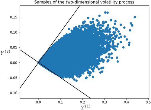
Notes. Plotted are all the points for every time step , i = 0,…,1,000 and all the samples. The decreasing black line is the line where the aggregated process , and the aggregated process is positive above that line. The nearly orthogonal second line cuts out a cone, which seems to give the actual domain of the process. Note that no samples actually lie outside the cone inscribed in the figure.
1.1. Main Contributions
The main question we are interested in can be summarized as follows:
What constitutes a suitable state space for the multifactor Markovian process in (1)?
Our main results in Theorem 2 and Corollary 1 establish that this state space can be represented as a linear transformation of , and we provide an explicit form for this transformation.
As a first application of this result, we prove that the weak simulation scheme for the rough Heston process proposed by Bayer and Breneis (2024) is well-defined in the sense that the variance process always stays nonnegative; see Section 3. In Section 4, we derive the corresponding pricing PDE on the transformed domain and solve it numerically by the finite element method after truncation of the domain. Naturally, knowing the PDE’s precise domain is crucial for accurate numerical approximations. Finally, in Section 5, we show how the explicit formula for the domain compares with general, abstract characterizations given in the literature by Abi Jaber and El Euch (2019a) and Cuchiero and Teichmann (2020).
1.2. Notation and Conventions
We denote by the i-th unit vector, which has a 1 in the i-th component and 0 in every other component; is the vector with 1 in every component; is the identity matrix; for a vector is the diagonal matrix with entries in the diagonal; and Throughout, italic letters a denote real numbers and bold letters denote vectors, where we write for the components of . An exception are stochastic processes, where components are denoted by (due to the time variable in the subscript).
2. State Spaces of the Multifactor Markovian Process
Fix . We consider the N-dimensional SDE
The aim of this section is to determine a state space of the multifactor process . That is, we want to determine a set such that for every starting value , there exists a -valued weak solution to (6)—that is, for all almost surely. In particular, the domain should be a subset of the half-plane to ensure nonnegativity of the aggregated weighted process , which for the specific case would correspond to the Volterra Process (1) for the weighted sum of exponential kernel K given in (1). As illustrated in Figure 1, and following the abstract characterizations of domains of (possibly infinite-dimensional) lifts of nonnegative Volterra processes in Abi Jaber and El Euch (2019a) and Cuchiero and Teichmann (2020), we suspect the domain to be a cone.
2.1. Main Result
We prove that the domain is a cone characterized by the set of admissible matrices, which is defined as follows.
A matrix is called admissible if it satisfies the following assumptions:
Q is invertible,
,
, where ,
for with .
We denote by the set of all admissible matrices.
Before stating our main theorem, we first show that the set of admissible matrices is nonempty by providing an explicit example of an admissible matrix. However, is not reduced to a singleton, as shown in Example 3 below.
The matrix given by
The proof is given in Section 2.4. □
We are now ready to state our main theorem that gives state spaces of the Multifactor Markovian Process (2).
Let be continuous functions satisfying the Linear Growth Condition (2) and the Boundary Conditions (1). Let be an admissible matrix in the sense of Definition 1 and suppose that
Set . Then, for each , there exists a -valued weak solution to (2).
The proof is given in Section 2.5. □
For the admissible matrix Q given in Theorem 1, the set corresponds to the set of such that and
The domain is not unique; see the appendix.
In practice—for instance, for the multifactor approximations of Volterra processes—we often have . Hence, it may be interesting to know whether as given in (2) is in . We treat this question in a slightly more general context in the following lemma.
Let Q be an admissible matrix and let satisfy (2). Then,
We prove the equivalent statement . First, note that
Recall that in linear algebra, an M-matrix is a square matrix with nonpositive off-diagonal entries and with eigenvalues whose real parts are nonnegative. Clearly, the matrix is an M-matrix: the nonpositivity of the off-diagonal entries holds by assumption, and its eigenvalues are (real and) positive, because it is just the matrix written in a different basis. Now, it is well-known that the inverse of an M-matrix has nonnegative entries (in fact, this property characterizes M-matrices). Therefore,
We remark that Condition (2) on can easily be dropped by using affine transformations of instead of linear ones. We give the specific details in the next corollary.
Let be continuous functions satisfying the Linear Growth Condition (2) and the Boundary Conditions (1). Let be an admissible matrix in the sense of Definition 1, and assume that . Let be chosen according to (2) with Define the set
Then, for any , there exists a -valued weak solution to (2).
Denote by a weak solution to
But this means that is a solution to (2) that stays in . The corollary follows immediately. □
We now give the specific result for the multifactor square-root process.
Consider the multifactor square-root model
Let Q be an admissible matrix, and assume that . Then,
2.2. Link with Nonnegative Volterra Processes
As an application of our result, one can obtain the existence of nonnegative solutions to Volterra equations with kernels of the Form (1). We note that such existence can be obtained by working directly on the level of the Volterra equation as done in Abi Jaber et al. (2019b, theorem 3.6 and example 3.7). Here, our result provides another alternative, as illustrated in the following corollary.
Let be continuous functions satisfying the Linear Growth Condition (2) and the Boundary Conditions (1). Let the kernel K be given by a weighted sum of exponentials as in (1). Then, for each , the Stochastic Volterra Equation (1) admits a nonnegative weak solution Y.
Fix , and let be such that . Let be chosen according to (2) with . Let be an admissible matrix—for instance, given by Theorem 1. Then, it follows from Lemma 1 that . Hence, , with given by (2). An application of Corollary 1, with the starting value , yields the existence of a -valued weak solution to the Equation (2). Thanks to the variation of constants formula, we can rewrite the equation in the form
Hence, for all , , which ends the proof. □
2.3. On Admissible Matrices for
In this section, we give examples of admissible matrices.
In the case , in Definition 1, conditions (2) and (3) imply that we are looking for a matrix of the form
Because , the last condition in Definition 1 is satisfied for any , and indeed, the domain is independent of the precise choice of q given by
For the case of the Multifactor Square-Root Process (2), the resulting sample paths of and are illustrated in Figure 2. Note that we chose the large maturity to give the process more time to explore its domain. Thereby, it is more clearly visible that the domain of is indeed than if we had set .
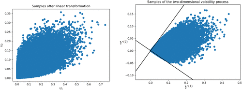
Notes. The black lines correspond to the hyperplanes in (3). The parameters used are and that is, is chosen to be proportional to .
For , a similar computation—relegated to the appendix due to its length—gives multiple choices of domains. See the appendix for details.
2.4. Proof of Theorem 1
In preparation for the proof, we introduce the matrix defined by
In Definition 1, conditions (2) and (3) are readily satisfied by construction. To argue condition (1), we will prove that R is actually the inverse of Q—that is, . Indeed, consider first the diagonal elements. Here, we have
Finally, we verify Definition 1, condition (4) by direct computations. First, it is easily verified that we have with
Now, let us compute
We have
2.5. Proof of Theorem 2
Fix an admissible matrix . The main idea of the proof is to reduce the study to the process and prove that its associated SDE admits an -valued solution.
We start by writing the SDE for . For this we first observe that due to (2), satisfies
Using the Definition 1 admissibility conditions (2) and (3), we have that and , which simplifies the equation to
Recall that is the N-th component of .
In order to prove Theorem 2, it suffices to prove that for each , there exists an -valued weak solution to (3). In particular, this would hold for any initial value of the form with , and setting , one obtains a -valued weak solution to (6) started at .
Hence, this boils down to establish that the set is stochastically viable with respect to Equation (3). Viability and invariance theory for stochastic differential equations have been extensively studied in the literature in various contexts and with different assumptions on the domain and the coefficients; we refer to Abi Jaber et al. (2019a), Da Prato and Frankowska (2004, 2007), and the references therein.
For the nonnegative orthant , the characterization in terms of the coefficients is very simple and means that, at boundary points, the diffusive coefficient has to be tangential to the boundary and the drift inward pointing. This is summarized in the following lemma.
Let be continuous satisfying the growth conditions
See for instance Da Prato and Frankowska (2007, example 2.7). □
We now proceed to the proof of Theorem 2.
It remains to apply Lemma 2 on Equation (3). For this, we define
Then, it readily follows from the continuity and growth conditions of b and that are also continuous with at most linear growth conditions. As for the Boundary Conditions (4), we fix such that for some .
For the diffusion term, we have
because if and if , where we used the boundary condition on in (3).For the drift term, we first observe that for the same reason , because thanks to the boundary condition on b in (1) and the fact that , so that we can write
This shows that the Boundary Conditions (4) are satisfied by , so that an application of Lemma 2 yields the existence of an -valued solution to (3) for any initial condition . In particular, it holds for the initial value with . Setting , one obtains a -valued weak solution to (2) started at and completes the proof of theorem. □
3. The Weak Scheme Is Cone-Preserving
In Section 2, we determined the state space of the multifactor square-root process given by (2). Assume now that we approximate the process using the weak simulation scheme proposed in Bayer and Breneis (2024). The goal of this section is to prove that the resulting approximation has the same viable domain as .
Let us first start by recalling the weak simulation scheme of Bayer and Breneis (2024). First, the SDE in (2) is split into two parts, one containing the drift and the other the diffusion. Denote by the solution at time h of the ordinary differential equation (ODE)
Then, the ODE (3) is linear and can hence be solved exactly. Therefore, the simulation scheme for the ODE is simply given by
We now recall the simulation scheme for the SDE (3). Note that the right-hand side of (3) is the same for all i. Thus, after multiplying (3) with , we get
Then, we define to be the random variable which is with probability , , noting, in particular, that .
We can now reconstruct an approximation from . Indeed, because the right-hand side of (3) is the same for all , the solution of (3) must be of the form
Hence, we set
Finally, we use Strang splitting to get the scheme
Let Q be an admissible matrix, and let be chosen according to (2). Then, for all and , the weak simulation algorithm described above satisfies . In particular, is well-defined.
Given and , we want to show that and . This will prove the theorem.
Consider first the algorithm . Recall that for some scalar random variable R. We have to verify that . The last component of this vector is given by
Next, consider the algorithm D. Recall that was given as the exact solution at time h of the ODE
Note that due to (2), for some . Defining , we have
In particular, we have to show that for with .
We start with . Here, we have
Of course, . Moreover, because of Definition 1, is a linear combination of where all the coefficients are nonnegative, with the exception of the coefficient of . However, because , this implies that .
Next, consider . Then,
As before, is again a linear combination of the , where all coefficients are nonnegative, with the exception of the coefficient of . But because , this implies that , proving the theorem. □
4. Solving PDEs
As an application of the domain, we want to solve PDEs. Recall that the multifactor square-root process is given by
Let be a “nice” payoff function. Then, we define the value function ,
Then, u satisfies the PDE
For numerical approximation, we then need to truncate the domain in space and impose appropriate boundary conditions. For simplicity, we will instead fabricate an appropriate source term such that the PDE has an explicit, given solution, which we then also impose as Dirichlet boundary condition on the boundary of the truncated domain.
Specifically, suppose that we want the exact solution to have the form
Plugging this formula into (4), we obtain a source term
|

Table 1. Parameters of the Stochastic Volatility of the Lifted Rough Heston Model Used for the Numerical Example
| N | ||||||
|---|---|---|---|---|---|---|
| 2 | 0.8 | 1.2 | 0.7 | |||
| 3 | 0.8 | 1.2 | 0.7 |
After truncation of the domain, we solve the PDE by the finite element method, using the package FEniCSx; see Baratta et al. (2023), and compare against the exact solution . In Table 2, we present the -errors on the truncated domain for three choices of truncated domains, each of side-length four:
|
Table 2. Errors over the Truncated Domain for the Approximate Finite Element Method (FEM) Solution to the PDE for in Dimension
| n | -error over the domain D | ||
|---|---|---|---|
| 4 | |||
| 8 | |||
| 16 | |||
| 32 | |||
| 64 | |||
| 128 | Inf | ||
| 256 | Inf | ||
| 512 | Inf | ||
| 1,024 | Inf | ||
Note. Inf, infinite.
, corresponding to a truncation in v-space which respects the cone-shaped actual domain of the process;
corresponding to a truncation in v-space, which respects neither the cone-shaped actual domain nor the nonnegativity condition;
corresponding to a domain truncation, which does not respect the cone-shaped actual domain in v-space but does respect the nonnegativity.
We use first-order Lagrange-type finite elements, with time-steps as well as mesh-size in each space dimension. (We refer to https://github.com/bayerc2/domain_multifactor_volterra for more details.)
We would like to emphasize that, although it might seem trivial to choose as the domain instead of, say, , this choice is based on correctly identifying the matrix Q and the domain , which is appropriately truncated here to . Without knowledge of Q, one would need to guess to truncate the domain, a task that becomes increasingly nontrivial in higher dimensions.
When nonnegativity of the variance process is preserved (cases 1 and 3), the numerical method empirically exhibits second-order convergence, with slightly smaller error when the computational domain is a subset of the invariant domain of the process (case 1). On the other hand, when nonnegativity of the variance process is not preserved on the computational domain (case 2), the error explodes due to the instability of the heat equation backward in time.
We also provide an example in dimension . In this case, we follow the construction outlined in the appendix. Note that the construction is not unique, so we tested different solutions to the system of inequalities leading to different admissible Q. Specifically, we choose
, , the default choice suggested in the appendix.
, , an admissible choice obtained by minimizing —related to the Lipschitz constant of the transformed drift—over all admissible choices of parameters a, b.
, , obtained by maximizing .
It turns out that there was no significant difference in the numerical results based on the different choices of transformation. Hence, we only report the results for the first choice. We report our numerical results in Table 3. Note that we had to limit the grid sizes due to the severely increased computational time. Hence, the accuracies reported may seem disappointing. However, note that the -error is unnormalized here. A normalized error would be obtained by dividing by the total volume of the (computational) domain, which is in this case. We observe an expected error decay when the domain is respected and highly erratic, diverging behavior when positivity is not preserved.
|
Table 3. Errors over the Truncated Domain for the Approximate FEM Solution to the PDE for in Dimension
| n | -error over the domain D | |
|---|---|---|
| 4 | ||
| 8 | ||
| 16 | ||
| 32 | ||
| 64 | ||
| 128 | ||
5. Remark on the Link Between the Sets and
In this section, we argue that the two abstract “invariance” sets that appeared in the literature in Abi Jaber and El Euch (2019a) and Cuchiero and Teichmann (2020) are equal. This part is valid for more general locally square-integrable kernels K beyond the weighted sum of exponential case.
We introduce the following notations. For suitable functions f, g and measure L, we denote their convolution by *:
The shift operator with maps any function f on to the function given by
If the function f on is right-continuous and of locally bounded variation, the measure induced by its distributional derivative is denoted , so that for all . By convention, df does not charge .
Two sets appeared so far in the literature to characterize the nonnegativity of solutions to stochastic Volterra equations:
Set of Cuchiero and Teichmann (2020, equation (4.7), definition 4.12, and theorem 4.17(i)):1
Here, is the resolvent of the second kind of the kernel defined bySet of Abi Jaber and El Euch (2019a, equations (2.4)–(2.5) and theorem 2.1):
where is the resolvent of the first kind of the kernel2
One can argue that the two sets are equal:
We note that the first line is exactly the condition that appears in the set . We sketch why is equivalent to the nonnegativity of for all , under suitable assumptions on the nonnegative kernel K (for instance, when K is a weighted sum of exponentials; see Abi Jaber and El Euch 2019a, and for precise conditions). The implication follows from Abi Jaber and El Euch (2019a, theorem A.2) with and therein. For the converse direction, fix and assume that . Clearly, , and from (5), we have
To conclude that , it suffices to note that the right-hand side tends to zero as , because in this limit (this follows from the Laplace transform of (8), given by , which goes to 0 as ).
In conclusion, the nonnegativity of the Linear Volterra Equation (8), for any , is equivalent to the condition that appears in , as well as the one that appears in , which shows that the two sets are equal.
In principle, to establish a link with our cone , one should restrict to kernels that are weighted sums of exponentials of the form
Then, the resolvents of the second kind and first kind for such kernels must be computed and plugged into the conditions defining the sets and . Even in dimension , this leads to highly cumbersome and nontrivial computations, and it is not clear how to explicitly determine a suitable domain, as, for instance, our cone , for from and . This makes the approach in the current paper particularly crucial.
Appendix. Invariant Domains in Dimension
We extend the calculations presented for in Example 3 to the three-dimensional case. We are looking for a matrix of the form
Note that there are some scaling invariances in the equation . We may multiply rows of Q with positive (!) constants without changing this condition. Hence, we restrict ourselves to
Note that this corresponds to the assumption that and are both positive. Indeed, if we chose one of these entries to be 0 or , we would fail to find an appropriate matrix Q.
Define the matrix , where we denote , and set and . Then,
This further implies for a that
One can verify that the lower bound is always smaller than the upper bound, proving that such an a exists. However, it is slightly simpler and perhaps more illustrative to prove that satisfies these inequalities. For the upper bound, this is trivial. For the lower bound, note that
Next, for b, we get the conditions
This time, we verify that is admissible. For the lower bound, this is clear. For the upper bound, note that
This again follows from the definition of c.
Hence, we have shown that we can choose and , yielding
Note that due to scaling invariance, the matrix
Consider now the specific example and Then, we get the conditions
Comparing to the previous discussion, we see that, indeed, and are admissible.
The corresponding plots for the multifactor square-root process are shown in Figure A.1. We give projections to two-dimensional planes, because this makes it easier to visually verify that the samples lie in . Furthermore, we give three different choices of , with the first two being admissible and the third not. Indeed, we see for the first two choices that the samples lie in , whereas this is not the case for the third choice.
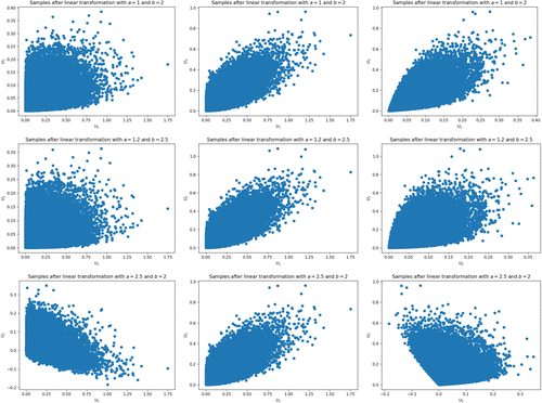
Note. The parameters used are and is chosen to be proportional to .
1 We point out that in Cuchiero and Teichmann (2020, equation (4.7)), the invariance condition is expressed on the initial values of the Markovian lift of the Volterra process. In our setting, we formulate the invariance property directly in terms of the Volterra process itself, with input curve . The connection between the two sets is made when one considers input curves of the form with the notations of Cuchiero and Teichmann (2020, equation (4.7)).
2 Under some suitable assumptions on the kernel (see Abi Jaber and El Euch 2019a, assumption (H1)), one can show that K admits a resolvent of the first kind such that is right-continuous and of locally bounded variation (see Abi Jaber and El Euch 2019a, remark B.3); thus, the associated measure that appears in the set is well defined.
References
- (2019) Lifting the Heston model. Quant. Finance 19(12):1995–2013.Google Scholar
- (2019a) Markovian structure of the Volterra Heston model. Statist. Probab. Lett. 149:63–72.Google Scholar
- (2019b) Multifactor approximation of rough volatility models. SIAM J. Financial Math. 10(2):309–349.Google Scholar
- (2019a) Stochastic invariance of closed sets with non-Lipschitz coefficients. Stochastic Processes Their Appl. 129(5):1726–1748.Google Scholar
- (2019b) Affine Volterra processes. Ann. Appl. Probab. 29(5):3155–3200.Google Scholar
- (2021) Linear-quadratic control for a class of stochastic Volterra equations: Solvability and approximation. Ann. Appl. Probab. 31(5):2244–2274.Google Scholar
- (2024) Approximation of stochastic Volterra equations with kernels of completely monotone type. Math. Comput. 93(346):643–677.Google Scholar
- (2013) Numerical integration of the extended variable generalized Langevin equation with a positive Prony representable memory kernel. J. Chem. Phys. 139(4):044107.Google Scholar
- (2023) DOLFINx: The next generation FEniCS problem solving environment. Preprint, submitted December 31, https://doi.org/10.5281/zenodo.10447666.Google Scholar
- (2023a) Markovian approximations of stochastic Volterra equations with the fractional kernel. Quant. Finance 23(1):53–70.Google Scholar
- (2023b) Weak Markovian approximations of rough Heston. Preprint, submitted September 13, https://arxiv.org/abs/2309.07023.Google Scholar
- (2024) Efficient option pricing in the rough Heston model using weak simulation schemes. Quant. Finance 24(9):1247–1261.Google Scholar
- (2007) Optimal approximations of power laws with exponentials: Application to volatility models with long memory. Quant. Finance 7(6):585–589.Google Scholar
- (1998) Fractional Brownian motion and the Markov property. Electronic Commun. Probab. 3:95–107.Google Scholar
- (2022) American options in the Volterra Heston model. SIAM J. Financial Math. 13(2):426–458.Google Scholar
- (2020) Generalized Feller processes and Markovian lifts of stochastic Volterra processes: The affine case. J. Evolution Equations 20(4):1301–1348.Google Scholar
- (2004) Invariance of stochastic control systems with deterministic arguments. J. Differential Equations 200(1):18–52.Google Scholar
- (2007) Stochastic viability of convex sets. J. Math. Anal. Appl. 333(1):151–163.Google Scholar
- (2019) The characteristic function of rough Heston models. Math. Finance 29(1):3–38.Google Scholar
- (2019) Strong convergence rates for Markovian representations of fractional Brownian motion. Preprint, submitted February 4, https://arxiv.org/abs/1902.01471v1.Google Scholar
- (2021) Second-order weak approximations of CKLS and CEV processes by discrete random variables. Mathematics 9(12):1337.Google Scholar
- (2025) A time-stepping deep gradient flow method for option pricing in (rough) diffusion models. Quant. Finance 25(12):2009–2020.Google Scholar