Disruptive Timing

1. Introduction

An extensive amount of literature examines disruptive innovation as a strategy for new entrants to outcompete established incumbents who struggle to respond (Christensen and Bower 1996, Adner and Zemsky 2005, Pacheco-de-Almeida 2010, Wu et al. 2014, Gans 2016, Almeida Costa and Zemsky 2021).¹ Although the definition and boundaries of what qualifies as disruptive innovation continue to be hotly debated, it is clear that this particular entry strategy does indeed occur and resonates practically with managers of both entrant and incumbent firms.

Despite the depth of work on disruptive innovation, extant research has not yet considered the role of timing in an entry strategy of disruptive innovation and thus, we argue, leaves out a critical mechanism for whether and when entrants “disrupt” incumbents. Our work characterizes the phenomenon whereby an incumbent firm offering an existing technology faces an entrant offering an alternative, potentially disruptive, technology. If the entrant then wins the market—because the incumbent stayed with the existing technology rather than switching to the alternative technology—one could say that the incumbent was “disrupted” by the entrant with its “disruptive technology.” From this general premise, we set out to unpack this phenomenon by providing a theoretical framework of disruptive innovation that accounts for the overlooked but critical element of timing, building on the insight from Gans (2016, p. 81) that “it’s all in the timing.” We draw upon an established literature that recognizes timing as fundamental for building competitive advantage (Lieberman and Montgomery 1988, Cirik and Makadok 2023) through assets with time-compression diseconomies (Pacheco-de Almeida and Zemsky 2007, Pacheco-de-Almeida 2010, Wibbens 2021) and competitive deterrence (Swinney et al. 2011, Hawk et al. 2013, Ruiz-Aliseda 2016).²

We develop an analytic model of disruptive innovation to examine the role of strategic timing. We model the entrant’s timing of entry with an alternative, potentially disruptive, technology and the endogenous timing of an incumbent response of switching from its existing technology to the alternative technology (if at all). These strategic timing decisions are informed by a micromodel of future payoffs, using a reduced-form approach that links value creation to firm payoffs based on a firm’s added value (Adner and Zemsky 2006, Adner et al. 2014, Ross 2014). As a critical feature, the model considers how disruption depends on both the exogenous and endogenous improvement trajectories of a potentially disruptive technology relative to an existing technology. Each technology exogenously improves from general technological advancements and secular shifts in customer preferences. But timing becomes especially strategic if we recognize that technology also improves endogenously: Firm-specific learning accrues to an entrant when it enters the market with its technology and the incumbent faces the sacrifice of forfeiting learning accumulated toward its existing technology if and when it switches.

Our model generates two key findings to advance our understanding of disruptive innovation. First, we find that the timing of the entrant is a strategic decision that affects whether disruption occurs at all by influencing the strategic timing of the incumbent’s response. Building on work by Adner and Zemsky (2005), who formalize the conditions to predict whether disruption occurs in a market, our model focuses on when disruption occurs as an endogenous consequence of strategic timing by an entrant and an incumbent. Whereas the existing understanding of disruption often assumes the entrant’s timing is exogenous, we identify scenarios in which the entrant benefits from strategically delaying—postponing entry into the market—and other scenarios where the entrant benefits from strategically rushing—preemptive entry into the market. These timing strategies make it more difficult for the incumbent to justify a response to prevent its own disruption.

Second, we characterize conditions under which the incumbent can eventually respond to and survive a potential disruptive technology, which is arguably the far more common outcome observed in practice than suggested by the original theory of disruptive innovation. We observe a scenario where the entrant enters the market with an immature disruptive technology and the incumbent intentionally waits and allows the entrant to capture market share rather than responding immediately. At initial glance, it would appear as if the incumbent was on a path to being disrupted. Rather, the incumbent is temporarily allowing itself to be self-displaced, a deliberate strategy proposed by Pacheco-de-Almeida (2010). But as enough time passes—such that the disruptive technology exogenously improves—the incumbent eventually switches to the disruptive technology and splits the market, coexisting with the entrant. Even though the incumbent may not get disrupted out of the market, the incumbent’s existing technology does get disrupted, and we take the view that this should be considered a form of disruption that has so far been overlooked.

To synthesize these findings on strategic timing in disruption, we propose the high-level typology framework presented in Table 1. To preview its implications, let us first consider its dimensions. The rows reflect the entrant’s decision: Strategically, an entrant with an alternative technology can either immediately enter the market at the earliest possible time (Race) or delay its entry to a later point in time (Dawdle). The columns reflect the incumbent’s decision: An incumbent may—as a best response to the entrant’s strategic choice we just described—choose to stay with its existing technology (No Response), or it can respond to the entrant by switching to the alternative technology either after waiting some time (Delayed Response) or immediately at the same time when the entrant appears (Immediate Response).

Table 1. Typology of Disruptive Timing

Organized by these dimensions, this framework characterizes the five distinct types of disruption that emerge as equilibrium outcomes of the model described in Section 3: Perfect Disruption, Postponed Disruption, Passing Disruption, Phased Disruption, and Partial Disruption. Later, we will return to the specifics of each type and illustrate their intuition by applying them to a number of case studies in markets like cloud computing, mobile devices, and artificial intelligence. The academic and popular literature generally interprets all disruption phenomena as just Perfect Disruption; accounting for timing allows us to go beyond just this one type and identify several novel but overlooked types of disruption, collectively embodying a more general view of disruption.

The paper proceeds as follows. Section 2 summarizes the conceptual background motivating our model. Section 3 specifies the model. Section 4 reports the findings. Section 5 provides further intuition and illustrative case studies to contextualize the findings. Section 6 concludes with a discussion of general contributions of this research, its relationship to the strategy literature and managerial practice, and its limitations.

2. Conceptual Background

The phenomenon now known as disruptive innovation has been a central theme in the study of technological change and strategy. Although the seminal work of Christensen and Bower (1996) popularized the term disruptive innovation, the origins of disruptive innovation can be traced back to Schumpeter (1934) and his notion of creative destruction. Foundational economic theories identify how incumbents facing the cannibalization of existing products have less incentive to invest in innovation (Arrow 1962, Reinganum 1983), even if doing so could protect market position (Gilbert and Newbery 1982). Beyond these economic incentives, organizational factors can also hinder incumbent adaptation to new technologies, including capability obsolescence (Tushman and Anderson 1986), architectural misalignment (Henderson and Clark 1990), managerial cognition (Tripsas and Gavetti 2000), and internal disagreement (Bresnahan et al. 2012, Gans 2024). Furthermore, the structure and dynamics of customer preferences for new technologies can also make disruption more likely (Adner 2002, Adner and Zemsky 2005).

Although these perspectives collectively advance our understanding of incumbent challenges in the face of a new technology, we address, instead, the role of strategic timing in disruptive innovation. We do so from the perspectives of the entrant originally bringing a new technology to market and of the incumbent deciding whether and when to respond. As critical work in this direction, Pacheco-de-Almeida (2010) examines how hypercompetitive environments and time-compression diseconomies make rapid innovation disproportionately costly for incumbents, influencing their timing decisions. Building on this work, we consider both exogenous technology improvement and endogenous firm-specific learning, along with barriers to entry and switching costs. We now consider three adjacent literatures—strategic timing, technology trajectories, and barriers to entry and switching—that serve as the foundation for our view of strategic timing in disruption.

2.1. Timing

A firm’s competitive advantage depends on how its timing positions it against competitors and aligns with the maturity of its technology ecosystem.

With respect to competitors, the literature documents a number of first-mover or early-mover advantages that come from entering the market to attain resources before competitors (Lieberman and Montgomery 1988, 1998). First, work on strategic factor markets argues that some assets can be rivalrous, in that the first firm to attain the resource can foreclose competitors from having the same asset (Adegbesan 2009, Chatain 2014, Asmussen 2015). For instance, relationships with customers, suppliers, and complementors in the ecosystem exhibit stickiness or lock-in, advantaging the firm that is first to reach those stakeholders (Joshi et al. 2009, Jia 2013, Ozcan and Hannah 2020). Second, the time-compression diseconomies view argues that building up a requisite stock of many assets requires time (Pacheco-de-Almeida 2010, Wibbens 2021); thus, early entry maintains a persistent advantage for those assets with time-compression diseconomies.

With respect to the ecosystem around a technology, extensive work on technology evolution implies that timing relative to the maturity of the context affects whether the firm can create value. Arriving too early to market—amidst great uncertainty (Klingebiel and Joseph 2016)—can leave a firm with neither prepared customers (Lee 2009) nor available complementors and suppliers (Bayus and Agarwal 2007, Suarez and Lanzolla 2007). At the other end, being too late in the market means the market may be saturated already with competitors who have built up the previously described advantages of being early (Swinney et al. 2011, Ruiz-Aliseda 2016).

These timing factors provide a basic logic for how our model conceptualizes timing strategy in the environment assumed by disruptive innovation theory. The timing of a disruptive technology entrant needs to balance first-mover advantage against the limitations of a market early on the S-curve. An incumbent firm already in the market with an existing technology has a decision on whether and when to switch to the same disruptive technology: This timing decision will additionally depend on the timing of the entrant.

2.2. Technology Trajectory

The trajectory of a technology’s improvement over time can vary as a function of exogenous-to-the-firm characteristics of the technology and the endogenous choice of a firm to enter with or switch to the technology.

Several exogenous-to-the-firm characteristics of a specific technology choice endow a technology with its own unique trajectory, that is, steeper or flatter. First, the trajectory can be determined by the general development of scientific and technological paradigms (Dosi 1982, Winter 1984). It can vary as a function of the time it takes to resolve general uncertainty and complexity (Peterson and Wu 2021). Second, technologies can vary in the rate over time that customers realize value, that is, customer demand (Zhou et al. 2015, Adner et al. 2016, Schmidt et al. 2016). Although a customer’s willingness-to-pay does depend on the performance level of the technology, the translation from technology to customer demand can exhibit discontinuous thresholds and decreasing marginal utility (Christensen 1997, Adner and Levinthal 2001). Third, the performance of a product based on a given technology also depends on the readiness of the external ecosystem, which the focal firm cannot fully control (Reisinger et al. 2021, Chatain and Plaksenkova 2023).

In addition, the exogenous technology trajectory needs to be considered along with firm-specific learning associated with that technology. Based on the endogenous choice of a firm to enter with or switch to that technology, a firm can improve on that technology via firm-specific learning (Cohen and Levinthal 1990, Schmidt and Keil 2013, Chen et al. 2018, Leiblein et al. 2023).³ Prior literature on other competitive implications of relative trajectories considers both the external technology trajectory and the firm-specific learning component (Rahmandad 2008, Balasubramanian and Lieberman 2010, Rahmandad 2012, Hawk et al. 2013). Despite the clear importance of firm-specific learning in strategy, most interpretations of disruptive innovation focus on the exogenous component of a technology trajectory, independent of a firm’s endogenous choice of that technology (Pacheco-de-Almeida 2010).

We model different improvement trajectories for a potential disruptive technology relative to an existing technology, where the trajectory of a technology consists of both an exogenous component and an endogenous firm-specific component. As we later show, whether and when disruption occurs depends on not just the aggregate trajectory of the disruptive versus existing technology but whether that improvement occurs exogenously—benefiting all potential firms deploying that technology—or via endogenous learning—a consequence of a firm’s strategic choice to offer that technology. A key consideration is how relative speed—how much faster is the exogenous improvement of the disruptive technology over the existing technology—compares to the incumbent’s rate of firm-specific learning in existing technology. When relative speed is fast, the disruptive technology must eventually become better than the existing technology. But when relative speed is slow, whether the disruptive technology becomes superior in the long term depends on the endogenous choice of firms to adopt it. In both situations, allowing for endogenous learning makes timing strategic, for both the entrant and the incumbent.

2.3. Barriers to Entry and Switching Costs

2.3.1. Entrant Barriers to Entry.

An entrant’s choice of whether and when to enter the market will depend on the barriers to entry it faces (Geroski 1995, Gans et al. 2002). Barriers to entry are vital in first-mover advantage research (Lieberman and Montgomery 1998), a key theoretical foundation for strategic timing. An incumbent already in the market would have ex ante built barriers to entry through prior fixed-cost investments, for example, research and development (R&D) or learning, manufacturing or distribution setup, marketing, control of key resources, and so on. To overcome these barriers, the entrant must incur the cost of mobilizing the same resources (Helfat and Lieberman 2002, Clough et al. 2019). We view barriers to entry as an important, but potentially neglected, consideration for when disruption by an entrant might actually occur.

We model an upfront fixed cost of entry, following Gans and Stern (2000), Chatain and Zemsky (2007), and Chatain and Mindruta (2017); we refer to this as the entrant fixed cost. Depending on the attractiveness of this starting position, an entrant may choose to never enter or at least wait before entering. One could imagine many scenarios where a potential disruptive technology exists, per se, but where we, as empirical observers, do not observe disruption happening because the disruptive technology entrant has not entered (yet).

2.3.2. Incumbent Switching Cost.

Switching costs are a critical factor in an incumbent’s ability to respond to a disruptive technology. Ghemawat (1991) conceptualizes switching costs as the repositioning costs that arise from revising prior commitments. These commitments enhance competitive advantage but simultaneously increase the difficulty of change. Thus, repositioning requires altering multiple interconnected activities (Menon and Yao 2017) in the course of retooling operations, reformulating products, rebranding, and so on (Makadok and Ross 2013). Switching costs also encompass investments in acquiring requisite resources or divesting burdensome overhead (Argyres et al. 2019).

Following Marx et al. (2014), we model incumbent switching costs as an upfront fixed cost paid by the incumbent to switch from the existing technology to the disruptive technology; we refer to this as the incumbent fixed cost. Of course, although switching costs certainly affect whether an incumbent can respond to a disruptive technology, our focus is on how the switching cost affects when the incumbent responds to the entrant.

3. Model

This section presents a game-theoretical model of timing decisions among firms in technology competition. Following the presentation approach of Pacheco-de Almeida and Zemsky (2007), Section 3.1 first provides the macro-structure of the game-theoretical model highlighting the firms’ timing decisions and interactions; we specify the timeline and state the payoff functions of the firms. Section 3.2 develops the microfoundation of the payoff functions, accounting for technology improvement, firm-specific learning, customer choice, and time discounting.

3.1. Timeline and Decisions

We model two firms, an incumbent $\mathcal{I}$ and a potential entrant $\mathcal{E}$, competing over a target market in a continuous-time game. Two possible technologies can be offered to the target market: an existing technology e and an alternative potentially disruptive technology, which we refer to as disruptive technology d. The incumbent firm starts in the market by initially offering the existing technology e. Meanwhile, the entrant may enter the market only with the disruptive technology d.⁴ In response to the entry, the incumbent could switch to the disruptive technology d.⁵ This interaction between the entrant and the incumbent determines how the firms split the market and earn their profits.

3.1.1. Timing Game.

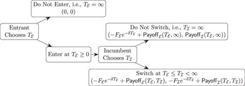
The incumbent and the potential entrant engage in a Stackelberg game where timing decisions are central. Currently enjoying monopoly profits with existing technology, the incumbent faces a potential entrant introducing a disruptive technology. By paying a fixed cost $F_{\mathcal{E}}\in {\mathbb{R}}_{\ge 0}$, the entrant can enter the market at any moment $t\ge 0$. The entry triggers the incumbent’s choice of whether and when to switch to the disruptive technology. If the incumbent decides to switch, it incurs a fixed cost $F_{\mathcal{I}}\in {\mathbb{R}}_{\ge 0}$. Let $T_{\mathcal{E}}\ge 0$ denote the entry time and $T_{\mathcal{I}}\ge T_{\mathcal{E}}$ denote the switch time. Moreover, we use $T_{\mathcal{E}}=\infty$ ($T_{\mathcal{I}}=\infty$) to capture the scenario where the entrant (incumbent) decides not to adopt the disruptive technology. Thus, $(T_{\mathcal{E}},T_{\mathcal{I}})$ represents the strategies of the firms.

3.1.2. Firm Payoffs.

Upon entry, the incumbent and the entrant accumulate profit over time. Specifically, let ${\mathrm{\Pi }}_{\mathcal{E}}(t|T_{\mathcal{E}},T_{\mathcal{I}})$ and ${\mathrm{\Pi }}_{\mathcal{I}}(t|T_{\mathcal{E}},T_{\mathcal{I}})$ denote the entrant’s and the incumbent’s instantaneous profits at time $t(\ge T_{\mathcal{E}})$ given $(T_{\mathcal{E}},T_{\mathcal{I}})$, respectively. We further denote ${\mathsf{\text{Payoff}}}_{\mathcal{I}}(T_{\mathcal{E}},T_{\mathcal{I}})={\int }_{T_{\mathcal{E}}}^{\infty }{\mathrm{\Pi }}_{\mathcal{I}}\left(t\right|T_{\mathcal{E}},T_{\mathcal{I}}) e^{-\delta t}\text{d}t$ and ${\mathsf{\text{Payoff}}}_{\mathcal{E}}(T_{\mathcal{E}},T_{\mathcal{I}})={\int }_{T_{\mathcal{E}}}^{\infty }{\mathrm{\Pi }}_{\mathcal{E}}\left(t\right|T_{\mathcal{E}},T_{\mathcal{I}}) e^{-\delta t}\text{d}t$ to be the discounted payoffs of the incumbent and the entrant, respectively, accrued over time after the entry, where $\delta \in {\mathbb{R}}^{+}$ denotes the instantaneous discount rate of time. Taking fixed costs into account, the entrant’s and the incumbent’s discounted profits are $-F_{\mathcal{E}}{e}^{-\delta T_{\mathcal{E}}}+{\mathsf{\text{Payoff}}}_{\mathcal{E}}(T_{\mathcal{E}},T_{\mathcal{I}})$ and $-F_{\mathcal{I}}{e}^{-\delta T_{\mathcal{I}}}+{\mathsf{\text{Payoff}}}_{\mathcal{I}}(T_{\mathcal{E}},T_{\mathcal{I}})$, respectively.

Each firm aims to maximize its own profit while anticipating the potential reactions of the opponent. Figure 1 illustrates the extensive form of the game.⁶ We aim to identify the subgame perfect Nash equilibrium for the game. To ensure the existence of an equilibrium and simplify the presentation, if multiple optimal decisions exist for either firm, we break the tie by favoring no change over change.

Intuitively, the higher the fixed costs, the more reluctant the firms would be to adopt the disruptive technology. Therefore, the timing decisions should be monotonically increasing with respect to the fixed costs. We formalize this intuition in the Online Appendix for general payoff functions.⁷ To generate additional insights, we need to specify the payoff functions. Here, we present the entrant’s and the incumbent’s discounted long-term payoff functions given the timing choice $(T_{\mathcal{E}},T_{\mathcal{I}})$ and complete the description of the game:

The following section elucidates the microfoundations of the aforementioned payoff functions by clarifying the notation and delineating the modeling choices.⁸

3.2. Microfoundations of the Payoff Functions

We now specify the micromodel of the firm payoff functions. First, Section 3.2.1 describes how firm timing decisions determine the exogenous and endogenous contribution of technology improvement to customer willingness to pay. Second, Section 3.2.2 links firms’ technology choices to customers’ willingness to pay and explains the customer choice model. Third, Section 3.2.3 takes a reduced-form approach to calculate the firms’ instantaneous payoffs based on their added value and integrates the payoffs over time to obtain the discounted long-term payoff functions.

3.2.1. Technological Improvement and Firm-Specific Learning.

Now, we model the relationship between the firms’ instantaneous profit and their technological strengths, as well as how technological improvement and firm-specific learning shape their respective technological strengths.

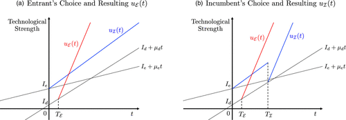
Let $u_i(t)$ denote the technological strength of firm $i(\in \{\mathcal{E},\mathcal{I}\})$ at time $t(\ge T_{\mathcal{E}})$. To capture the effects of technological improvement and firm-specific learning, we further decompose $u_i(t)$ into two components: $u_i(t)=u_k(t)+u_{i,k}(t)$, where firm i adopts technology option $k\in \{d,e\}$ at time t. For simplicity, we assume both components are linear functions of time t. That is, the technology-specific component $u_k(t)=I_k+{\mu }_{k}t$ for $k\in \{d,e\}$, where ${\mu }_k\in {\mathbb{R}}^{+}$ and $I_k\in {\mathbb{R}}^{+}$ capture the rate of technological improvement over time and the intercept at time 0 for option k, respectively. For the firm-specific component, we have $u_{\mathcal{I},e}(t)={\mathcal{\ell }}_{e}t$ for $0\le t\le T_{\mathcal{I}}$ and $u_{i,d}(t)={\mathcal{\ell }}_d(t-T_i)$ for $t\ge T_i$ ($i\in \{\mathcal{E},\mathcal{I}\}$), where ${\mathcal{\ell }}_k\in {\mathbb{R}}^{+}$ denotes the firm-specific learning of option $k\in \{d,e\}$.

Figure 2 illustrates how the firms’ technological strengths change over time. In Figure 2(a), the entrant choice of entry time determines $u_{\mathcal{E}}(t)$. Figure 2(a) also illustrates $u_{\mathcal{I}}(t)$ under no switch, whose slope is ${\mu }_e+{\mathcal{\ell }}_e$ capturing both the technological improvement and firm-specific learning. Similarly, the slope of $u_{\mathcal{E}}(t)$ is ${\mu }_d+{\mathcal{\ell }}_d$. In Figure 2(b), the incumbent needs to determine the switch time $T_{\mathcal{I}}\ge T_{\mathcal{E}}$, which consequently decides $u_{\mathcal{I}}(t)$. If $T_{\mathcal{E}}<T_{\mathcal{I}}$, upon switching the incumbent would always lag behind the entrant in valuation due to the firm-specific learning.⁹

In summary, we have the following expressions for the technological strength $u_i(t)$:

It turns out that this linear technological improvement setup implies a bifurcated structure as long as the firm’s instantaneous profit can be written as a function of the technological strength difference between the firm and its opponent (i.e., ${\mathrm{\Pi }}_{\mathcal{E}}(t|T_{\mathcal{E}},T_{\mathcal{I}})={\alpha }_{\mathcal{E}}\mathrm{\Pi }(u_{\mathcal{E}}(t)-u_{\mathcal{I}}(t))$ and ${\mathrm{\Pi }}_{\mathcal{I}}(t|T_{\mathcal{E}},T_{\mathcal{I}})={\alpha }_{\mathcal{I}}\mathrm{\Pi }(u_{\mathcal{I}}(t)-u_{\mathcal{E}}(t))$ for some function $\mathrm{\Pi }$ and constant ${\alpha }_{\mathcal{E}},{\alpha }_{\mathcal{I}}\in [0,1]$), where $\mathrm{\Pi }$ is monotonically increasing in the technological strength difference.¹⁰ When the existing technology dominates the disruptive technology in terms of improvement speed (i.e., ${\mu }_d-{\mu }_e<{\mathcal{\ell }}_e$), the time difference in adoption increases as the entrant time increases; when the disruptive technology dominates the existing technology (i.e., ${\mu }_d-{\mu }_e>{\mathcal{\ell }}_e$), the time difference in adoption decreases as the entrant time increases. We formally document this result as Proposition C.2 in Online Appendix C.2.

3.2.2. Customer Choice Model.

Now we model the relationship between the technological strength and willingness to pay. Notice that customers would have choices after the entry, that is, $t\ge T_{\mathcal{E}}$. Let $U_i(t)$ denote the customer’s willingness to pay for the offering from firm $i(\in \{\mathcal{E},\mathcal{I}\})$ at time t. We assume that $U_i(t)$ can be written as

where the deterministic term $u_i(t)$ is firm i’s technological strength and ${ϵ}_i(t)$ is a random term (McFadden 1974).

We assume that customers face a choice problem and would only match up with one of the firms. Adopting the well-known multinomial logit (MNL) model (Anderson et al. 1992, Train 2009), we assume the random term ${ϵ}_i(t)\sim$ i.i.d. Gumbel(0,$\beta$) for $i\in \{\mathcal{E},\mathcal{I}\}$, where $\beta \in {\mathbb{R}}^{+}$ is the scale parameter. In particular, $\beta$ represents the degree of customer heterogeneity (Makadok and Ross 2013): The bigger the value of $\beta$, the more diverse the customers are in their willingness to pay; as $\beta$ approaches zero, their willingness to pay converges to the same value.

We choose the MNL model for its solid theoretical foundation and wide applications in many fields, such as engineering, business, and economics. The MNL model is also known for its simplicity—here, we only introduce one more parameter $\beta$ to capture customer heterogeneity. Because the MNL model adopts a probabilistic approach for the customer choice, the expected market share and value creation functions are twice differentiable. In contrast, a linear segmentation model uses a linear combination of continuous variables to create segments, and often, one needs to handle the corner solutions explicitly.

We define value creation as willingness to pay minus variable cost. Under the MNL model, a given firm $i(\in \{\mathcal{E},\mathcal{I}\})$ wins a random customer when the realization of the random term (${ϵ}_i$) of the customer utility is such that firm i’s value creation for this customer is the highest. Without loss of generality, we normalize all the firm’s variable costs to be zero, so value creation equals willingness to pay. Thus, the expected instantaneous overall value created by both firms at time $t(\ge T_{\mathcal{E}})$ equals

where $\gamma$ is Euler’s constant ($\gamma \approx 0.5772$) (Anderson et al. 1992, Chu and Wang 2015).¹¹

3.2.3. Profit Function and Market Share.

We follow a reduced-form approach to determine firm payoffs, an approach taken in strategy research by Adner and Zemsky (2006), Adner et al. (2014), and Ross (2014) that builds on earlier work by Brandenburger and Stuart (1996, 2007), Brandenburger and Nalebuff (1996), and Stuart (2002). Given that our model of disruptive timing is primarily concerned with the implications of value creation (from the improvement of technology over time) for competitive decisions in timing, we take this reduced-form approach to intentionally abstract away from details of value capture. We assume that each firm’s payoff is a fraction of its added value, which is defined as the difference between the value creation with and without the focal firm’s participation.¹²

Based on the value creation expression, we can express the expected instantaneous added value by firm $i(\in \{\mathcal{E},\mathcal{I}\})$ at time $t(\ge T_{\mathcal{E}})$ as the difference between the overall value creation with and without its participation:

Let ${\alpha }_i\in (0,1]$ be the fraction of the added value that firm i captures, which can be viewed as a proxy for bargaining ability. Then, the expected instantaneous profit of firm i is ${\alpha }_i·\beta \ln \left(\frac{{\sum }_{j\in \{\mathcal{E},\mathcal{I}\}}{e}^{\frac{u_j(t)}{\beta }}}{{\sum }_{j\ne i}{e}^{\frac{u_j(t)}{\beta }}}\right)={\alpha }_i\beta \ln \left(1+e^{\frac{u_i(t)-{\sum }_{j\ne i}{u}_j(t)}{\beta }}\right)$ for time $t\ge T_{\mathcal{E}}$.¹³ That is, the function $\mathrm{\Pi }$ that links the relative technological strength and the instantaneous profit can be characterized as $\mathrm{\Pi }\left(x\right)=\beta \hspace{0.17em}\ln (1+e^{{\displaystyle \frac{x}{\beta }}})$.

Recall that $\delta$ denotes the discount rate of time. Moreover, by (1) and (2), we have

The entrant’s and the incumbent’s long-term payoffs after the entry are

We also consider the market shares of the firms over time. Before the entry, the incumbent controls the market. Let $s_{\mathcal{E}}(t)$ and $s_{\mathcal{I}}(t)$ denote the entrant’s and the incumbent’s market shares at time $t(\ge T_{\mathcal{E}})$, representing the probability of a customer choosing either firm, respectively. Under the MNL model, $s_{\mathcal{E}}(t)=\frac{e^{\frac{u_{\mathcal{E}}(t)}{\beta }}}{e^{\frac{u_{\mathcal{E}}(t)}{\beta }}+e^{\frac{u_{\mathcal{I}}(t)}{\beta }}}=\frac{1}{1+e^{\frac{u_{\mathcal{I}}(t)-u_{\mathcal{E}}(t)}{\beta }}}$.¹⁴ Therefore,

The market share of the incumbent is $s_{\mathcal{I}}(t)=1-s_{\mathcal{E}}(t)$.

To recap, our game-theoretical model of disruptive timing models the entrant’s timing of market entry with disruptive technology and the endogenous timing of an incumbent response of switching from its existing technology to the disruptive technology (if at all). A micromodel of payoffs for future time periods informs these timing decisions.¹⁵

4. Analysis and Main Results

This section presents the findings of the model. We characterize firms’ timing decisions and the conditions under which each type of disruption occurs (Table 1).

We find that the relative speed of exogenous improvement in the disruptive technology versus the existing technology (${\mu }_d-{\mu }_e$) plays a critical role in determining firm behavior. As such, we report findings organized by two scenarios of relative speed (${\mu }_d-{\mu }_e$) compared with the rate of firm-specific learning by the incumbent for its existing technology (${\mathcal{\ell }}_e$). The slow relative-speed scenario occurs when the incumbent’s endogenous learning for the existing technology dominates the exogenous advantage of the disruptive technology over the existing technology (${\mu }_d-{\mu }_e\le {\mathcal{\ell }}_e$). The fast relative-speed scenario occurs when the disruptive technology’s inherent exogenous advantage over the existing technology dominates the possible endogenous learning about the existing technology (${\mu }_d-{\mu }_e>{\mathcal{\ell }}_e$).

Table 2 previews our findings. We report the equilibrium behavior for each outcome, the relative-speed scenarios where the equilibrium appears, and the entrant’s market share over time (as derived in Proposition 5).

Table 2. Summary of Findings

Sections 4.1 and 4.2 analyze the slow and the fast relative-speed scenarios and the disruption outcomes observed in each, respectively. Section 4.3 illustrates how the disruption outcomes vary by the relative speed and how firm profit and market share performance evolve over time for each disruption outcome. Section 4.4 summarizes several extensions to the base model, verifying the robustness and generality of our insights. The Online Appendix contains the proofs for all the propositions and details the model extensions.

4.1. Slow Relative Speed (${\mu }_d-{\mu }_e\le {\mathcal{\ell }}_e$)

We now consider the slow relative-speed scenario of ${\mu }_d-{\mu }_e\le {\mathcal{\ell }}_e$. We first consider the incumbent’s best response given the entrant’s timing to unpack the strategic interaction between firms. We then characterize possible equilibrium outcomes and illustrate how they vary based on the fixed costs.

4.1.1. Incumbent’s Best Response.

We first show that the incumbent has only two possible responses: either never switch to the disruptive option ($T_{\mathcal{I}}=\infty$), or switch to the disruptive option right after the entrant’s entry ($T_{\mathcal{I}}=T_{\mathcal{E}}$). Recall that $T_{\mathcal{I}}^{\mathsf{\text{BR}}}(T_{\mathcal{E}})$ denote the incumbent’s optimal switching time given the entry time $T_{\mathcal{E}}$. Proposition 1 formalizes our observation.

Proposition 1

(Best Response Under Slow Relative Speed). When ${\mu }_d-{\mu }_e\le {\mathcal{\ell }}_e$, $T_{\mathcal{I}}^{\mathsf{\text{BR}}}(T_{\mathcal{E}})\in \{T_{\mathcal{E}},\infty \}$. Moreover, the incumbent’s best response follows a threshold policy: There exists $\tau \in {\mathbb{R}}_{\ge 0}{\displaystyle \cup \{+\infty \}}$ such that switching immediately is the incumbent’s best response if $T_{\mathcal{E}}<\tau$, and never switching is the incumbent’s best response if $T_{\mathcal{E}}\ge \tau$. Furthermore, if $F_{\mathcal{I}}\ge \frac{{\alpha }_{\mathcal{I}}\beta \ln (2)}{\delta }$, $\tau =0$ and $T_{\mathcal{I}}^{\mathsf{\text{BR}}}(T_{\mathcal{E}})=\infty$; if $\tau >0$, $\tau$ strictly increases with ${\mu }_d-{\mu }_e$ and $\beta$. In addition, if the equilibrium decision $T_{\mathcal{E}}^{*}\in (0,\infty )$, $T_{\mathcal{E}}^{*}=\tau$.

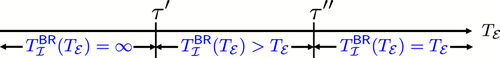
To visualize Proposition 1, Figure 3 illustrates the incumbent’s timing choice as a function of entry time when $0<\tau <\infty$. The threshold $\tau$ is such that the incumbent’s profit is the same under either switching immediately or never switching (which is uniquely determined by equation $-F_{\mathcal{I}}{e}^{-\delta \tau }+{\mathsf{\text{Payoff}}}_{\mathcal{I}}(\tau ,\tau )={\mathsf{\text{Payoff}}}_{\mathcal{I}}(\tau ,\infty )$). The incumbent opts not to switch by the tie-breaking rule.

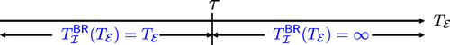
Proposition 1 implies that the entrant can discourage the incumbent from adopting disruptive technology by postponing market entry. Under the slow relative-speed scenario, the slope of the disruptive trajectory is less steep than that of the incumbent’s current technology, which combines both the existing trajectory and firm-specific learning As such, the later the incumbent can switch, the less attractive the disruptive technology appears. In essence, by delaying its entry, the entrant assists in entrenching the incumbent with the existing technology, thereby deterring the switch to the disruptive technology. Furthermore, the higher the customer heterogeneity, the longer the entrant needs to wait for the incumbent to be entrenched with the existing technology.¹⁶

4.1.2. Equilibrium Outcomes.

We now study the equilibrium timing decisions for the slow relative-speed scenario. Specifically, Proposition 2 fully characterizes the entrant’s and the incumbent’s timing decisions with respect to $F_{\mathcal{E}}$ and $F_{\mathcal{I}}$ for the slow relative-speed scenario.

Proposition 2

(Outcome of Slow Relative Speed). When ${\mu }_d-{\mu }_e\le {\mathcal{\ell }}_e$, there exists $F_{\mathsf{\text{slow}}}^{\prime }(F_{\mathcal{I}})$, $F_{\mathsf{\text{slow}}}^{″}(F_{\mathcal{I}})$, ${\widehat{F}}_{\mathcal{I}}(\le \frac{{\alpha }_{\mathcal{I}}\beta \ln (2)}{\delta })$, and ${\tilde{F}}_{\mathcal{I}}\le {\widehat{F}}_{\mathcal{I}}$ such that, when $F_{\mathcal{I}}\ge {\widehat{F}}_{\mathcal{I}}$,

$$(T_{\mathcal{E}}^{*},T_{\mathcal{I}}^{*})=\{\begin{array}{ll}(0,\infty ),\hfill & \hspace{1em}\hspace{1em}\hspace{1em}\hspace{1em}\text{for} F_{\mathcal{E}}<F_{\mathsf{\text{slow}}}^{″}\hfill \\ (\infty ,\infty ),\hfill & \hspace{1em}\hspace{1em}\hspace{1em}\hspace{1em}\text{for} F_{\mathcal{E}}\ge F_{\mathsf{\text{slow}}}^{″}.\hfill \end{array}$$

When ${\tilde{F}}_{\mathcal{I}}<F_{\mathcal{I}}<{\widehat{F}}_{\mathcal{I}}$,

$$(T_{\mathcal{E}}^{*},T_{\mathcal{I}}^{*})=\{\begin{array}{ll}(\tau ,\infty ),\hfill & \hspace{1em}\hspace{1em}\hspace{1em}\hspace{1em}\text{for} F_{\mathcal{E}}<F_{\mathsf{\text{slow}}}^{″}\hfill \\ (\infty ,\infty ),\hfill & \hspace{1em}\hspace{1em}\hspace{1em}\hspace{1em}\text{for} F_{\mathcal{E}}\ge F_{\mathsf{\text{slow}}}^{″}.\hfill \end{array}$$

When $F_{\mathcal{I}}\le {\tilde{F}}_{\mathcal{I}}$ and $F_{\mathcal{I}}<{\widehat{F}}_{\mathcal{I}}$,

$$(T_{\mathcal{E}}^{*},T_{\mathcal{I}}^{*})=\{\begin{array}{ll}(0,0),\hfill & \hspace{1em}\hspace{1em}\hspace{1em}\hspace{1em}\text{for} F_{\mathcal{E}}\le F_{\mathsf{\text{slow}}}^{\prime }\hfill \\ (\tau ,\infty ),\hfill & \hspace{1em}\hspace{1em}\hspace{1em}\hspace{1em}\text{for} F_{\mathsf{\text{slow}}}^{\prime }<F_{\mathcal{E}}<F_{\mathsf{\text{slow}}}^{″}\hfill \\ (\infty ,\infty ),\hfill & \hspace{1em}\hspace{1em}\hspace{1em}\hspace{1em}\text{for} F_{\mathcal{E}}\ge F_{\mathsf{\text{slow}}}^{″}.\hfill \end{array}$$

Moreover, $F_{\mathsf{\text{slow}}}^{\prime }(F_{\mathcal{I}})$ is a decreasing function of $F_{\mathcal{I}}$ on $[0,{\tilde{F}}_{\mathcal{I}}]$, and $F_{\mathsf{\text{slow}}}^{″}(F_{\mathcal{I}})$ is an increasing function of $F_{\mathcal{I}}$ on $[0,{\widehat{F}}_{\mathcal{I}}]$. Furthermore, $T_{\mathcal{E}}^{*}$ and $T_{\mathcal{I}}^{*}$ (weakly) increase with $F_{\mathcal{E}}$ and $T_{\mathcal{I}}^{*}$ (weakly) increases with $F_{\mathcal{I}}$.

It is worth noting that Proposition 2 holds as long as Proposition 1 holds. That is, the monotone structure of the incumbent’s best response function, and not the specific payoff functional forms, drives this result for the slow relative scenario.

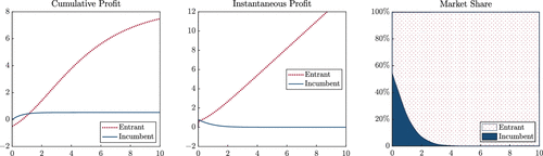
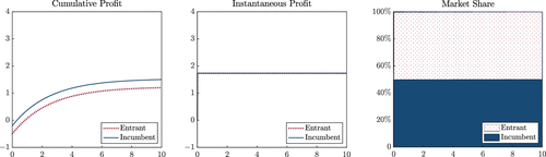
Proposition 2 shows that there are three possible equilibrium outcomes: $(0,0)$, $(0,\infty )$, and $(\tau ,\infty )$. Equilibrium outcome $(0,0)$ corresponds to Partial Disruption, under which both firms adopt the disruptive technology immediately and the disruptive technology overtakes the existing technology. Equilibrium outcome $(0,\infty )$ corresponds to Perfect Disruption or Pretend Disruption, depending on whether the disruptive technology can dominate the existing technology in the long run (i.e., the sign of $({\mu }_d-{\mu }_e)-({\mathcal{\ell }}_e-{\mathcal{\ell }}_d)$). Specifically, when the relative speed of the disruptive trajectory is sufficiently slow (${\mu }_d-{\mu }_e<{\mathcal{\ell }}_e-{\mathcal{\ell }}_d$), equilibrium outcome $(0,\infty )$ corresponds to Pretend Disruption, whereby the entrant races to enter the market ($T_{\mathcal{E}}^{*}=0$) and the incumbent never responds by switching to the disruptive trajectory ($T_{\mathcal{I}}^{*}=\infty$). Just based on these entry timing decisions, intuitively, one might interpret this outcome as the incumbent being disrupted. Interestingly, however, because the relative speed of the disruptive trajectory is too slow, although the incumbent never switches to the disruptive trajectory, the entrant eventually loses the market. That is why we term this scenario as Pretend Disruption, which will be illustrated in Section 4.3. The familiar Perfect Disruption can occur only when the relative speed of the disruptive trajectory is not too slow (${\mu }_d-{\mu }_e>{\mathcal{\ell }}_e-{\mathcal{\ell }}_d$) (so that Pretend Disruption does not occur).

Equilibrium outcome $(\tau ,\infty )$ (with $\tau >0$) corresponds to Postponed Disruption, which happens as the entrant strategically times its entry to deter the switch. Under the slow relative-speed scenario, if one assumes that the incumbent never switches, the entrant’s optimal timing choice would be either now or never (i.e., 0 or $\infty$). The entrant chooses a positive entry time only to deter the incumbent from switching.

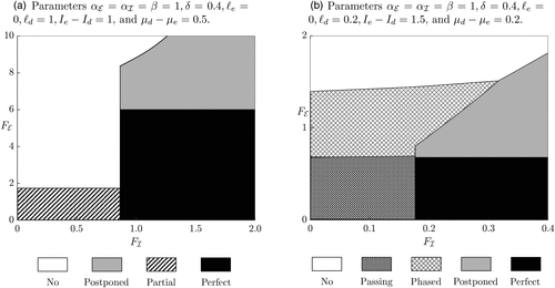
To visualize Proposition 2, Figure 4 illustrates how the entrant’s fixed cost of entry $F_{\mathcal{E}}$ and the incumbent’s fixed cost of switching $F_{\mathcal{I}}$ impact the equilibrium strategy for the slow relative-speed scenario (i.e., ${\mu }_d-{\mu }_e\le {\mathcal{\ell }}_e$). Specifically, Figure 4(a) illustrates the case where the relative speed of the disruptive trajectory is sufficiently slow (${\mu }_d-{\mu }_e<{\mathcal{\ell }}_e-{\mathcal{\ell }}_d$), and Figure 4(b) illustrates the case where the relative speed is slow but not too slow (${\mathcal{\ell }}_e-{\mathcal{\ell }}_d<{\mu }_d-{\mu }_e\le {\mathcal{\ell }}_e$). Although Figure 4 makes specific parameter assumptions for illustrative purposes, the general implications of Proposition 2 hold regardless of these choices.

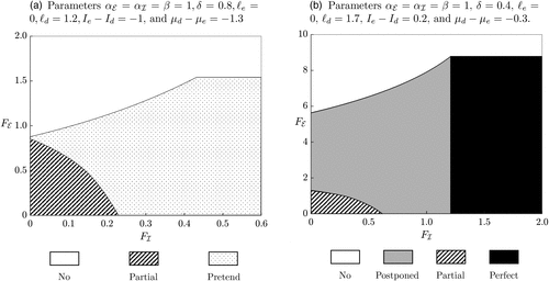
In both Figure 4, (a) and (b), when the entrant’s fixed cost is prohibitively high, the blank region represents the no-disruption equilibrium, that is, $T_{\mathcal{E}}^{*}=T_{\mathcal{I}}^{*}=\infty$. When the entrant’s fixed cost is low, as the incumbent’s fixed cost increases, we observe the equilibrium outcome shifts from Partial Disruption to Pretend Disruption in Figure 4(a) and shifts from Partial Disruption to Postponed Disruption and to Perfect Disruption in Figure 4(b). As the incumbent fixed cost increases, the incumbent becomes “weak” and more reluctant to switch. In Figure 4(b), in particular, as the incumbent’s fixed cost increases, the entrant can delay its entry to deter the incumbent from switching, resulting in Postponed Disruption. As the incumbent’s fixed cost increases further, the incumbent becomes even “weaker” and would not switch whatsoever. The entrant need not delay the entry anymore, resulting in Perfect Disruption.¹⁷

4.2. Fast Relative Speed (${\mu }_d-{\mu }_e>{\mathcal{\ell }}_e$)

We now consider the fast relative-speed scenario, that is, ${\mu }_d-{\mu }_e>{\mathcal{\ell }}_e$. We first consider the incumbent’s best response given the entrant’s timing to unpack the strategic interaction between firms. We then characterize possible equilibrium outcomes corresponding to the disruption types and illustrate how they vary based on the fixed costs.

4.2.1. Incumbent’s Best Response.

In contrast to slow relative speed, the incumbent’s timing decision is more nuanced, as the incumbent may choose to switch after the entrant’s entry. Recall that $T_{\mathcal{I}}^{\mathsf{\text{BR}}}(T_{\mathcal{E}})$ denotes the incumbent’s optimal switching time given the entry time $T_{\mathcal{E}}$.

Proposition 3

(Best Response Under Fast Relative Speed). When ${\mu }_d-{\mu }_e\ge {\mathcal{\ell }}_e$, the incumbent’s best response follows a two-threshold policy: There exists ${\tau }^{\prime }\le {\tau }^{″}$ (${\tau }^{\prime },{\tau }^{″}\in \mathbb{R}{\displaystyle \cup \{+\infty \}}$) such that never switching is the incumbent’s best response if $T_{\mathcal{E}}\le {\tau }^{\prime }$, switching with a delay is the incumbent’s best response if ${\tau }^{\prime }<T_{\mathcal{E}}<{\tau }^{″}$, and switching immediately is the incumbent’s best response if $T_{\mathcal{E}}\ge {\tau }^{″}$. Moreover, $T_{\mathcal{I}}^{\mathsf{\text{BR}}}(T_{\mathcal{E}})$ strictly decreases with $T_{\mathcal{E}}$ and ${\mu }_d-{\mu }_e$ when ${\tau }^{\prime }<T_{\mathcal{E}}<{\tau }^{″}$. In addition, if the equilibrium decision $T_{\mathcal{E}}^{*}\in [{\tau }^{″},\infty )$, $T_{\mathcal{E}}^{*}={\tau }^{″}$.

To visualize Proposition 3, Figure 5 illustrates the incumbent’s timing as a function of entry time when $0<{\tau }^{\prime }<{\tau }^{″}<\infty$. Although the incumbent’s best response monotonically increases in the entry time under the slow relative-speed scenario, under the fast relative-speed scenario it monotonically decreases before increasing.

Proposition 3 implies that the entrant can discourage the incumbent from switching to the disruptive technology by accelerating its entry. Under the fast relative-speed scenario, the slope of the exogenous improvement trajectory for the disruptive technology is steeper than the combined exogenous and firm-specific learning trajectory of the existing technology for the incumbent. As such, if the entrant enters at a late time, the incumbent can abandon its existing technology and switch to the disruptive one. By entering the market early, the entrant can take advantage of firm-specific learning, whereas the incumbent prioritizes its returns from the existing technology. The incumbent may then forgo its opportunity to switch altogether. Thus, the entrant may delay or even deter the incumbent’s switch by preemptively entering the market.

4.2.2. Equilibrium Outcomes.

We now study the equilibrium timing decisions for the fast relative-speed scenario: Proposition 4 fully characterizes the entrant’s and the incumbent’s timing decisions with respect to $F_{\mathcal{E}}$ and $F_{\mathcal{I}}$.

Proposition 4

(Outcome of Fast Relative Speed). When ${\mu }_d-{\mu }_e>{\mathcal{\ell }}_e$, there exists ${\widehat{F}}_{\mathcal{E}}$, $F_{\mathsf{\text{fast}}}^{\prime }(F_{\mathcal{I}})$, $F_{\mathsf{\text{fast}}}^{″}(F_{\mathcal{I}})$, ${\widehat{F}}_{\mathcal{I}}(\le \frac{{\alpha }_{\mathcal{I}}\beta \ln (2)}{\delta })$, and ${\tilde{F}}_{\mathcal{I}}\le {\widehat{F}}_{\mathcal{I}}$ such that when $F_{\mathcal{I}}\ge {\widehat{F}}_{\mathcal{I}}$,

$$(T_{\mathcal{E}}^{*},T_{\mathcal{I}}^{*})=\{\begin{array}{ll}(0,\infty ),\hfill & \hspace{1em}\hspace{1em}\text{for} F_{\mathcal{E}}\le {\widehat{F}}_{\mathcal{E}}\hfill \\ (T_{\mathcal{E}}^{*},\infty ),\hfill & \hspace{1em}\hspace{1em}\text{for} {\widehat{F}}_{\mathcal{E}}<F_{\mathcal{E}}\le F_{\mathsf{\text{fas}}{\mathsf{t}}^{\prime }}\hfill \\ (T_{\mathcal{E}}^{*},T_{\mathcal{I}}^{*}),\hfill & \hspace{1em}\hspace{1em}\text{for} F_{\mathsf{\text{fas}}{\mathsf{t}}^{\prime }}<F_{\mathcal{E}}<F_{\mathsf{\text{fas}}{\mathsf{t}}^{″}}\hfill \\ (\infty ,\infty ),\hfill & \hspace{1em}\hspace{1em}\text{for} F_{\mathcal{E}}\ge F_{\mathsf{\text{fas}}{\mathsf{t}}^{″}},\hfill \end{array}$$

where, in the second case, $T_{\mathcal{E}}^{*}>0$ and, in the third case, $0<T_{\mathcal{E}}^{*}<T_{\mathcal{I}}^{*}<\infty$.

When ${\tilde{F}}_{\mathcal{I}}<F_{\mathcal{I}}<{\widehat{F}}_{\mathcal{I}}$,

$$(T_{\mathcal{E}}^{*},T_{\mathcal{I}}^{*})=\{\begin{array}{ll}(0,T_{\mathcal{I}}^{*}),\hfill & \hspace{1em}\hspace{1em}\text{for} F_{\mathcal{E}}\le F_{\mathsf{\text{fast}}}^{\prime }\hfill \\ (T_{\mathcal{E}}^{*},T_{\mathcal{I}}^{*}),\hfill & \hspace{1em}\hspace{1em}\text{for} F_{\mathsf{\text{fast}}}^{\prime }<F_{\mathcal{E}}<F_{\mathsf{\text{fast}}}^{″}\hfill \\ (\infty ,\infty ),\hfill & \hspace{1em}\hspace{1em}\text{for} F_{\mathcal{E}}\ge F_{\mathsf{\text{fast}}}^{″},\hfill \end{array}$$

where, in the first case, $0<T_{\mathcal{I}}^{*}<\infty$ and, in the second case, $0<T_{\mathcal{E}}^{*}<T_{\mathcal{I}}^{*}<\infty$.

When $F_{\mathcal{I}}\le {\tilde{F}}_{\mathcal{I}}$ and $F_{\mathcal{I}}<{\widehat{F}}_{\mathcal{I}}$,

$$(T_{\mathcal{E}}^{*},T_{\mathcal{I}}^{*})=\{\begin{array}{ll}(0,0),\hfill & \hspace{1em}\hspace{1em}\text{for} F_{\mathcal{E}}<F_{\mathsf{\text{fast}}}^{\prime }\hfill \\ (\infty ,\infty ),\hfill & \hspace{1em}\hspace{1em}\text{for} F_{\mathcal{E}}\ge F_{\mathsf{\text{fast}}}^{\prime }.\hfill \end{array}$$

Similar to the slow relative-speed scenario, Proposition 4 holds as long as Proposition 3 holds. That is, the structure of the incumbent’s best response function, and not the payoff functional forms, drives this result in the fast scenario.

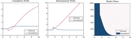
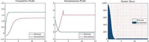
Proposition 4 shows that we may ignore the possibility that the entrant delays and the incumbent switches immediately and focus on five possible equilibrium outcomes: $(0,0)$, $(0,T_{\mathcal{I}}^{*})$, $(0,\infty )$, $(T_{\mathcal{E}}^{*},T_{\mathcal{I}}^{*})$, and $(T_{\mathcal{E}}^{*},\infty )$. Equilibrium outcome $(0,0)$ corresponds to Partial Disruption, under which both firms adopt the disruptive technology immediately and the disruptive technology overtakes the existing technology. Equilibrium outcome $(0,T_{\mathcal{I}}^{*})$ corresponds to Passing Disruption—a disruption type that exists only under the fast relative-speed scenario—under which the entrant races to enter and the incumbent switches with a delay. Equilibrium outcome $(0,\infty )$ corresponds to Perfect Disruption under the fast relative-speed scenario. Equilibrium outcome $(T_{\mathcal{E}}^{*},T_{\mathcal{I}}^{*})$ corresponds to Phased Disruption, under which the entrant enters with a delay and the incumbent switches with a further delay. Equilibrium outcome $(T_{\mathcal{E}}^{*},\infty )$ corresponds to Postponed Disruption. The last two types of equilibria warrant further elaboration.

Phased Disruption exists only under the fast relative-speed scenario. Recall that under the slow relative-speed scenario, if one assumes that the incumbent never switches, the entrant’s optimal timing choice would be either now or never (i.e., zero or $\infty$). This is no longer true under the fast relative-speed scenario. For intuition, consider a setting in which the disruptive technology is inferior at time 0 but improves quickly over time. In such a case, the entrant would ideally prefer waiting for the disruptive technology to be more mature before entering the market; that is, the entrant’s optimal timing would be positive (if the fixed cost is intermediate). Moreover, the incumbent would switch with a delay at equilibrium if the incumbent’s fixed cost is not too low.

The entrant may also deter the incumbent from switching by strategically choosing the entry time, resulting in Postponed Disruption, just like what we have under the slow relative-speed scenario, but for a completely different reason. Under the fast relative-speed scenario, the earlier the entry and more firm-specific learning the entrant can enjoy for the disruptive technology, the later the switch time the incumbent would choose. Therefore, to move away from Phased Disruption that accommodates the incumbent and move into Postponed Disruption that deters the incumbent, the entrant enters preemptively, a strategic behavior that exists only under the fast relative-speed scenario.

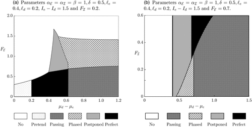
To visualize Proposition 4, Figure 6 illustrates how the entrant’s fixed cost of entry $F_{\mathcal{E}}$ and the incumbent’s fixed cost of switching $F_{\mathcal{I}}$ impact the equilibrium strategy for the fast relative-speed scenario (i.e., ${\mu }_d-{\mu }_e>{\mathcal{\ell }}_e$). Although Figure 6 makes specific parameter assumptions for illustrative purposes, the general implications of Proposition 4 hold regardless.

In Figure 6, in the bottom-left corner (i.e., when the fixed costs of both firms are low), the entrant rushes to adopt the disruptive technology, resulting in either Partial Disruption (Figure 6(a)) or Passing Disruption (Figure 6(b)). In the right part of the figures (i.e., when the incumbent’s fixed cost is high), it is possible to deter the incumbent from switching. We have Perfect Disruption, Postponed Disruption, and possibly Phased Disruption. The entry time increases as the entrant’s fixed cost increases. Unlike the slow relative-speed scenario, delaying the entry would not deter the incumbent, and it is in the entrant’s best interest to adopt disruptive technology immediately (at $T_{\mathcal{E}}=0$) when the entrant’s fixed cost is low. Moreover, in Figure 6, (a) and (b), the equilibrium outcome shifts from Partial Disruption and Passing Disruption to Perfect Disruption, respectively, as the incumbent’s fixed cost increases. These results occur because, as the incumbent’s fixed cost increases, the incumbent becomes “weak” and reluctant to switch. When the entrant’s fixed cost is prohibitively high, the blank region represents the no-disruption equilibrium ($T_{\mathcal{E}}^{*}=T_{\mathcal{I}}^{*}=\infty$).

4.3. Performance Outcomes

This section first presents how equilibrium disruption outcomes vary with the relative speed. We then illustrate the firm profits and market shares over time for each equilibrium outcome.

Figure 7 adopts the parameters from Figure 6(b) to illustrate how the equilibrium outcome varies with relative speed. In Figure 7(a), for very slow relative speed, the possible outcomes are Pretend Disruption or no disruption at all, depending on the entrant’s fixed cost. As the relative speed becomes moderately slow, Pretend Disruption disappears, and we observe Perfect Disruption and Postponed Disruption, under which the incumbent chooses not to switch. As the relative speed becomes moderately fast, Phased Disruption appears. Then, for very fast relative speed, Passing Disruption appears as the entrant rushes to enter the market. Figure 7(a) also shows that, as the entrant’s fixed cost increases, the entry time increases. Figure 7(b) illustrates that, as the incumbent’s fixed cost increases, the incumbent is more likely to get deferred or even deterred.

We can also characterize the instantaneous profits and market shares over time under various disruption types. The following proposition presents the results formally.

Proposition 5

(Market Share). (1) If the incumbent switches ($0\le T_{\mathcal{E}}^{*}\le T_{\mathcal{I}}^{*}<\infty$), both the entrant and the incumbent achieve constant market shares from $t=T_{\mathcal{I}}^{*}$ onward. (2) If the incumbent does not respond ($0\le T_{\mathcal{E}}^{*}<\infty ,T_{\mathcal{I}}^{*}=\infty$), the entrant’s market share decreases monotonically and converges to 0% when ${\mu }_d-{\mu }_e<{\mathcal{\ell }}_e-{\mathcal{\ell }}_d$; it remains constant over time when ${\mu }_d-{\mu }_e={\mathcal{\ell }}_e-{\mathcal{\ell }}_d$; and it increases monotonically and converges to 100% when ${\mu }_d-{\mu }_e>{\mathcal{\ell }}_e-{\mathcal{\ell }}_d$. The rate of convergence decreases with customer heterogeneity $\beta$.

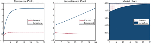
We now present the firms’ cumulative and instantaneous profits and market shares over time for each equilibrium outcome. Cumulative profit captures total discounted profits accrued over time, whereas instantaneous profit captures the rate of profits generated at each specific moment in time. Documenting both measures of profit helps to illustrate the underlying tension of disruption for incumbent firms: A current decision to switch to the disruptive technology has major positive effects on instantaneous profit in future periods, but when discounted back to the current periods and considered cumulatively, those profits appear relatively small. Figures 8–11 are created under the slow relative-speed scenario, whereas Figures 12 and 13 are created under the fast relative-speed scenario.

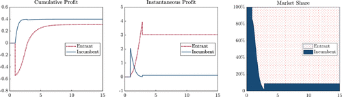
These figures provide intuition for how each plays out over time and how they might appear to an empirical observer. In Pretend Disruption (Figure 8), the entrant captures market share upon entry, seemingly portending a disruption of the incumbent, but the entrant ultimately fails to secure a stable market share and loses it all. In Perfect Disruption (Figure 9) and Postponed Disruption (Figure 10), the entrant grows share over time to eventually capture the entire market from the incumbent. In Partial Disruption (Figure 11), the firms split the market immediately and in perpetuity. In Passing Disruption (Figure 12) and Phased Disruption (Figure 13), the entrant enters and grows market share significantly as the incumbent loses much of its market share—but when the incumbent later switches to the disruptive technology, it recovers some market share back, albeit relatively little because of the entrant’s advantage from accumulating firm-specific learning. As the incumbent switches with a significant delay, the time-discounted associated fixed cost is negligible in the cumulative profit graph.

4.4. Model Extensions

We examine several model extensions to the base model to verify the robustness and generality of our insights. First, we relax the assumption that the entrant must enter only with the disruptive technology, allowing it to alternatively adopt the existing technology. Second, we consider the possibility that the incumbent can switch to the disruptive technology even before the entrant enters, potentially deterring disruption preemptively. Third, we incorporate the role of complementary assets, allowing the incumbent to have an ongoing product advantage (or disadvantage) when switching to the existing technology. Moreover, we explore a setting where the incumbent can offer both the existing and disruptive technologies simultaneously. Lastly, we examine an alternative model with a different microfoundation, where a noncooperative price-setting game determines firm profits. Across all these extensions, although the timing choices and market dynamics adjust, our fundamental conclusions about how strategic timing shapes disruption remain robust. We report these findings in the Online Appendix.¹⁸

5. Model Applications

We now interpret the model and its implications by translating each of the main outcomes predicted by the model (Table 1) to the real-life context of several recent and forward-looking case studies.¹⁹ Although we do not and cannot necessarily claim that our model is the only explanation of these examples, we merely intend to demonstrate that the theoretical predictions can plausibly reflect reality. In addition, these examples facilitate the translation of the theoretical findings for use by general managers and practicing strategists.

5.1. Perfect Disruption

The base case of Perfect Disruption (Figure 9) describes the scenario whereby the entrant enters immediately with the disruptive technology and the incumbent remains with its existing technology, unable to justify switching to the disruptive technology. We view this scenario as representing disruption as it is conventionally understood by scholars and managers. Many examples of disruption in the literature could be conceived of as Perfect Disruption: smaller disk drives from Seagate disrupting larger drives from IBM (Christensen 1997) or digital photography disrupting the analogue film of Polaroid (Tripsas and Gavetti 2000).

Our model shows that moderate, and not fast, exogenous improvements in the disruptive technology relative to the existing technology make Perfect Disruption more likely and more dangerous. In the model, a much more rapid exogenous improvement of a disruptive technology does not necessarily lead to incumbent failure: As illustrated in Figure 4, if the entrant faces high barriers to entry (low upfront fixed cost of entry) and the incumbent has low switching costs (low upfront fixed cost of switching), the entrant may not enter the market at all, or the incumbent may successfully adopt the new technology. Instead, a particularly dangerous scenario for the incumbent arises when the disruptive technology exogenously improves at a moderately slow rate. In the examples above, it took as long as a decade or more for the threats to materialize. Even if the incumbent’s fixed cost of switching is low, an extended period during which the disruptive technology remains inferior can lead the incumbent to become entrenched in its existing technology due to endogenous improvements. As a result, the incumbent forgoes the potential endogenous improvements in the disruptive technology, which instead accrue to the entrant.

5.2. Postponed Disruption

Our novel notion of Postponed Disruption (Figure 10) describes the scenario where an entrant strategically delays entry and the incumbent does not ever respond. Although this scenario generates the same observable outcome as Perfect Disruption, the strategic implication for the entrant is distinct. The disruption of the incumbent is not just a function of exogenous characteristics of the market and competitors: Through strategic timing, the entrant can actually cause the incumbent to be disrupted when, absent strategic timing, the incumbent would not be disrupted.

The occurrence of Postponed Disruption in the slow relative speed scenario best illustrates the intuition (Figure 4(b)).²⁰ When the incumbent faces a high fixed cost to switch—and the entrant’s fixed cost is not unreasonably high—the incumbent will of course often end up in Perfect Disruption. But if the incumbent’s fixed cost is low enough to make switching feasible, then the entrant’s timing becomes critical. Anticipating that the incumbent can respond, the entrant should strategically delay entry. This delay not only allows the disruptive technology to exogenously mature but, critically, allows the incumbent to accumulate experience with its existing technology. The entrant’s delay entrenches the incumbent in its existing technology, making a future switch less attractive for the incumbent. By strategically forgoing profits in early periods, the entrant impairs the flexibility of the incumbent.

In our view, delayed entry plays a critical role in an entrant’s ability to disrupt an incumbent more often than is first apparent. Although we cannot always infer from any real-world example whether there was a strategic intent by the entrant in its late entry, timing still matters for the eventual outcome, regardless of intent. Consider the market for content delivery network (CDN) services, which allow websites to efficiently and rapidly distribute content globally through a geographically distributed network of servers. Founded in 1998, Akamai defined the CDN business with its hardware-defined networking technology. Over more than 20 years, the incumbent Akamai built a global network of specialized hardware around the world that provides its customers with scalable content delivery.²¹

At the same time, an alternative (and potentially disruptive) technology for CDN would have been software-defined networking: using commodity hardware and writing software that does much of the work that would otherwise be addressed in the (specialized) hardware. More than 10 years after the software-plus-commodity-hardware approach became well-known, Cloudflare entered the market with software-defined networking technology. Cloudflare used commodity hardware—which over time became more powerful than the specialized hardware—and created all of the functionality of a CDN in software.²²

In 2025, Akamai still does not appear to be able to justify switching to the disruptive technology of software-defined networking. Instead, it is doubling down on its original strategy: Its recent acquisitions suggest that it plans to just sell more products to customers still locked into its original CDN network rather than switching to the newer CDN technology needed to compete for the future. To survive in the CDN market in the future, Akamai would have to decide to commit resources toward pivoting to software-defined networking. However, what protects Cloudflare today is that Akamai, more than a decade into its investment into its original technology, is far too enmeshed in its hardware-defined networking CDN technology to switch to the now superior software-defined networking.

Our view is that if software-defined networking technology had emerged as a threat earlier in the history of Akamai, it is possible that Akamai would have pursued building their network around that technology instead of sticking with hardware-defined networking exclusively. Based on that assumption, it would have made sense for Cloudflare to strategically delay entry to deter and block retaliation from Akamai. That said, there is a major caveat here: we cannot infer whether Cloudflare intentionally delayed with this purpose or if exogenous factors led to Cloudflare entering when it did. But late entry definitely gave Cloudflare this competitive benefit. More generally, distinguishing Postponed Disruption from Perfect Disruption requires proving strategic intention, and this is a fundamental limitation to any sort of ex post observation of disruption.

5.3. Passing Disruption

In Passing Disruption (Figure 12), the entrant immediately enters the market with its disruptive technology, and the incumbent does not immediately respond and instead waits some time before eventually switching to the disruptive technology. Despite the early fundamental weakness of the disruptive technology, the entrant strategically enters the market early to get first-mover advantage, making it less attractive for the incumbent to respond. On the other hand, the incumbent deliberately waits, choosing to be self-displaced (Pacheco-de-Almeida 2010). But as enough time passes—such that the disruptive technology exogenously improves to become attractive enough for the incumbent—the incumbent eventually switches to the disruptive technology and gains back (some) of the market, coexisting with the entrant. Akin to the logic underlying the option value of waiting (Cassiman and Ueda 2006, Sakhartov 2017), this scenario highlights deliberate strategic timing by the incumbent but in the competitive context.

Passing Disruption can occur only when relative speed is fast (Figure 6). Moreover, both the entrant’s fixed cost and the incumbent’s fixed cost of switching need to be low. The entrant needs it to be acceptably costly to enter when the disruptive technology is immature, and it anticipates an eventual response from the incumbent. Thus, the entrant seeks to build some first-mover advantage against the incumbent before that happens; the longer the entrant waits, the easier it will be for the incumbent to respond. For the incumbent, the fast exogenous improvement of the disruptive technology and a low fixed cost mean that it will eventually be attractive to switch even as it forgoes its own firm-specific learning.

We can apply the concept of Passing Disruption to understand what is happening in the market for Internet search engines as the potentially disruptive technology of generative AI chatbots comes into play. For two decades, Google dominated the business of search with a “traditional” technology of an indexed database monetized with display advertising. OpenAI entered the market with its ChatGPT chatbot in 2022, based on a potentially disruptive technology of a generative artificial intelligence (AI) transformer model monetized through subscriptions. ChatGPT soon became the fastest-growing software application of all time by gaining more than 100 million users in its first two months, all while accumulating data as the first mover in bringing generative AI chatbot technology to market. ChatGPT and the generative AI technology were widely perceived as a threat to Google Search. Although OpenAI is often publicly credited with launching the AI boom of the 2020s, Google had in fact long been a pioneer in generative AI, having actually invented the transformer in 2017. Google clearly delayed switching its search engine to generative AI technology, and, even as the threat of ChatGPT keeps growing, Google continued to avoid fully switching over (Wu et al. 2023, Wu and Yang 2025).

Although the public conversation often describes Google as a slow incumbent unaware of the risk of being disrupted by ChatGPT and generative AI, we propose that one could also view the situation through the lens of Passing Disruption. Since 2017 and up to at least 2025, generative AI continued to be an immature technology economically unattractive in its own right.²³ If Google immediately switched search to generative AI in response to OpenAI’s entry, Google would have forgone tens or even hundreds of billions of dollars in profit. Therefore, in the short term, it is arguably rational for Google to accommodate ChatGPT and limit its own switch to generative AI. The real question is what Google might do in the long term. By any measure, Google has the know-how and resources to make the switch. In our view, the critical question is when: The switch makes more sense after the generative AI technology exogenously matures—for example, variable costs fall as chips improve over time—and after OpenAI has captured “enough” market share from Google. Although we cannot be certain whether Google will eventually mount an effective generative AI response, our key point is that it is too soon to declare Google a victim of Perfect Disruption. While it is happening, Perfect Disruption and Passing Disruption appear the same to an observer; only years or decades after the fact can we know which was realized.

5.4. Phased Disruption

In Phased Disruption (Figure 13), the entrant delays entry, and the incumbent waits some time but does eventually switch. The intuition of the incumbent response in Phased Disruption is the same as in Passing Disruption. However, here the entrant delays entry to allow the disruptive technology to exogenously improve to the point where it can better justify incurring its upfront fixed cost of entry but while preserving some first-mover advantage against the incumbent; that is, it still strategically enters early. To illustrate, we apply this logic to a possible example in the market for high-end smartphones, or more precisely, folding-screen smartphones. The concept of a foldable device dates back as least as early as Nokia’s “Morph” concept in 2008, which for Samsung would have been way too early to enter given the lack of supporting technology. At the same time, Samsung as the entrant needs to anticipate the possible reaction of Apple, the dominant player in the high-end market, and ensure it builds enough of an advantage before Apple eventually offers its own folding-screen device. It was known that Apple was also (and still is) exploring folding screen technology.

Samsung waited for years, but in 2019, it made the decision to be first to market with its Galaxy Fold device, even though the technology and its supporting ecosystem were still weak. The product distributed to reviewers in April 2019 was widely criticized and even ridiculed, and yet Samsung still decided to rush it to market in September 2019 with serious deficiencies.²⁴ This widely panned first-generation product was a massive financial loss.²⁵

But Samsung continued to persist—by 2025 it was now in its seventh generation of the Galaxy Fold—and it has clearly accumulated firm-specific experience, as shown by the obvious improvements over product generations.²⁶ Rumors continue to abound among industry insiders that Apple will eventually launch its own folding-screen smartphone. But Apple’s timeline appears to keep getting pushed further and further back. Through the lens of our model, Samsung’s first-mover advantage allowed it to improve on the technology to put it ahead of what Apple would consider launching. In turn, this accumulated advantage actually has the effect of deterring a response from Apple, particularly as it has also improved its conventional smartphone. Thus, we have to consider the following thought experiment: If Samsung had not preemptively launched folding-screen phones, would Apple have in fact launched folding-screen phones earlier (or even already)? Obviously we cannot know that for certain, but this is what our model would suggest. At minimum, Apple certainly has the ability to compete in this market, and it is definitely still plausible that it will.

5.5. Partial Disruption

In Partial Disruption (Figure 11), the entrant enters immediately, but the incumbent responds immediately by switching to the disruptive technology, and they split the market. Although the incumbent and the entrant end up coexisting, the existing technology is “disrupted” and replaced by the disruptive technology in the market, and the incumbent is “partially” disrupted as it loses significant market share. The intuition for this scenario is straightforward: Simply, the incumbent’s upfront fixed cost of switching is low enough that it can easily respond to the entrant and do so immediately (Figures 4 and 6).

An example of Partial Disruption occurred in the retail brokerage market in recent years. The incumbent retail brokerages like Charles Schwab traditionally operated on a commission-based business model; by charging customers for each trade they make, this model disincentivizes customers from making many trades. Founded in 2013, Robinhood introduced the concept of commission-free trading, whereby there would be no apparent fee paid by retail users; instead, Robinhood monetized via payment for order flow, for example, charging market makers and hedge funds like Citadel for the right to fulfill trades requested by Robinhood users, an opportunity valuable to high-frequency traders who may “front-run” customers. Not having to pay a commission drew new users and incentivized more trades.

Incumbents certainly faced a nontrivial decision of whether to switch. In addition to the loss in direct revenue from giving up the commission, accepting payment for order flow would conflict with their desired image of acting in the best interest of their retail clients, a reputation that took years to build. But this transition was far less than insurmountable: Charles Schwab and others adopted the commission-free trading model, and they continue to operate in 2025, coexisting with Robinhood.²⁷

6. Concluding Discussion

In this article, we develop a stylized theoretical model to advance a broader understanding of disruptive innovation by accounting for strategic timing. Our model of disruptive timing considers both the exogenous and endogenous improvement rates of technologies. First, we show that timing is a strategic choice of the entrant that can determine the response and survival of the incumbent. Second, we characterize the conditions under which the incumbent can respond to and survive against a potentially disruptive entrant, which is arguably a far more common outcome in practice than getting pushed out of the market. The model and these two findings together allow us to offer a high-level framework characterizing a typology of distinct types of disruption that paints a broader picture of disruption beyond how it is traditionally understood. We now highlight the contributions of this research toward the literature on the phenomenon of disruption—identifying the role of strategic timing—and for managerial practice—drawing out actionable implications of the theory—and conclude by identifying opportunities for future research.

6.1. Disruptive Innovation and Strategic Timing

Our analytical model intends to broaden the conceptual understanding of the disruption phenomenon by closely examining and highlighting the critical role of timing. We examine both the strategic timing of the entrant’s choice to enter and the timing of the incumbent’s endogenous response (if at all). Importantly, our game-theoretical approach describes how disruption can occur when managers make fully rational decisions, and it does not need to depend on the assumption of low-quality or complacent management. In particular, we argue that the occurrence of disruption—both whether and when the incumbent gets disrupted—can be a function of the strategic timing of the entrant: For a given technology, entering at a specific time can be a deciding factor in preventing or delaying the incumbent from responding. In those situations, the entrant’s timing is a necessary input into whether disruption occurs. Thus, we take the view that a complete understanding of disruptive innovation should account for the role of timing.

Examining disruption while accounting for timing allows us to move beyond the binary categorization of being disrupted or not, offering a richer characterization of the strategic decisions and performance outcomes for both the incumbent and the entrant that fall under our broader view of disruption. Our typology proposes that disruption can come in multiple flavors: Perfect, Postponed, Passing, Phased, and Partial Disruption. To date, most of the conversation around disruption typically concerns what we refer to as Perfect Disruption; the other four types are novel to this study. We argue that a broader view of disruption should consider all these cases. In particular, we show that, under many conditions, an incumbent can respond to an entrant with a disruptive technology by switching to the disruptive technology itself, and the market ends up in a coexistence scenario where both the incumbent and the entrant survive. Our view is that disruption as a general concept should encompass both when the incumbent gets disrupted (losing some or all of the market) or if its existing technology gets disrupted (switching to the disruptive technology of the entrant) even as the incumbent firm survives in the marketplace.

6.2. Managerial Application of Strategic Timing

Our theoretical framework can be interpreted to generate a number of actionable insights for managers, both of potential disruptive entrants and incumbents facing potential disruption.

6.2.1. Entrant Strategy.

For a potential entrant with a disruptive trajectory, the key insight is that it should make an explicit decision on whether to immediately enter or instead to strategically delay entry. This choice will determine whether it can achieve the ultimate success of forcing the incumbent out of the market. As Perfect Disruption and Passing Disruption illustrate, an entrant should be prepared to enter as soon as possible, even before the market or technology is fully ready, because preemptive entry can have the effect of foreclosing or delaying a response from the incumbent. Also, in Postponed Disruption and Phased Disruption, the entrant can strategically delay entry if doing so causes the incumbent to entrench itself in its existing technology, curtailing its response to the eventual entry. Thus, even for an entrant confident in the eventual value of its disruptive technology, strategically timing its entry is still necessary to win and disrupt the incumbent out of the market.

6.2.2. Incumbent Strategy.

Although most of our exposition around the model focuses on understanding the strategic timing of the entrant, we can also infer some best practices for an incumbent facing potential entrants with disruptive strategies. There are many scenarios where the incumbent can survive by switching to the disruptive technology and where the entrant can be deterred altogether from entering. Thus, the incumbent should foster the conditions where either of these ends up being the case by taking preventive action. First, the incumbent can invest in reducing its switching cost if it were to ever need to switch to the disruptive technology. By publicly advertising and committing to these investments, the incumbent could plausibly deter the entrant from even entering and thereby subvert any future need to actually switch strategies. Second, the incumbent can build barriers to entry that increase the fixed cost of entry for the disruptive entrant. For instance, the incumbent could lobby for burdensome regulations or contractually lock up infrastructure and resources necessary for the disruptive technology. Third, to the extent that the incumbent can affect the trajectory of its existing technology, the incumbent can make investments that advance the broader ecosystem and technology that underlie its existing technology to reduce the gap in the relative trajectories between its existing technology and the potentially disruptive technology.

6.3. Limitations and Future Research

As with any study, our work has limitations that open several fruitful avenues for future research and improvement beyond the current model. First, our model employs a reduced-form approach to determine firm payoffs based solely on relative value creation (i.e., added value) that abstracts away from the nuances of value capture. Although this simplification enables progress on understanding strategic timing in disruption, it leaves out important value capture dynamics (Gans and Ryall 2017, Montez et al. 2018). For instance, one could specify a more detailed model of bargaining in a cooperative game (MacDonald and Ryall 2004, Bennett 2013, Grennan 2014), or one could allow pricing to emerge from product-market competition as in a noncooperative game (Marshall and Parra 2020). In the present model, a firm captures an exogenously determined fraction of its added value (${\alpha }_i$), and future work could allow a firm to make an endogenous choice or investment to alter their bargaining power against customers (Chatain and Zemsky 2007, Almeida Costa and Zemsky 2021), which may reveal multiple equilibria. Furthermore, future work could allow for intertemporal strategic pricing; for example, an incumbent could cut prices to defend its market share, possibly leading to more gradual or delayed technological switching than the current model would predict.

Second, we model the exogenous and endogenous components of a technology trajectory simply as linear functions of time. In the digital world, and especially for platform and AI technologies, technology improves from network effects and learning curves, which follow curvilinear patterns with increasing or decreasing returns, respectively. Modeling these patterns is a critical next step, particularly in conjunction with the intertemporal pricing behavior mentioned above: In these types of markets, firms may use pricing to manage short-term market share to influence long-term outcomes. Pursuing this may require an alternative modeling approach or a combination (Hannah et al. 2021). Third, although our study focuses on the competition between an entrant and an incumbent, an incumbent may also choose to license the technology from an entrant (“borrow”) (Gans and Stern 2000, Panico 2017, Cabral and Pacheco-de Almeida 2018), acquire the entrant (“buy”) (Bryan and Hovenkamp 2020, Callander and Matouschek 2022), or learn from one another (Giustiziero et al. 2019). Fourth, we analyze continuous customer heterogeneity, whereas prior works such as Christensen and Bower (1996) and Adner and Zemsky (2005) emphasize discrete customer segments. One could explore how disruptive timing plays out under discrete or other representations of customer heterogeneity (Adner and Snow 2010). Fifth, we model the firm as a unitary actor, but in reality, a firm is a set of distinct stakeholders with their own incentives and beliefs, engaging in complex interactions (Vroom 2006). We view our theory of disruptive timing as complementary to the rich literature on organizational perspectives of disruption (Gans 2024). Sixth, we model rational firms making decisions based on economic profits, but, of course, managers and investors can have behavioral biases or alternative preferences. Our work provides a basis for exploring the implications: For instance, short-termist investors may influence managers into underinvesting in R&D for new technologies (Benner 2007).

All that said, this study purposefully emphasizes a core model tailored for capturing the basic intuition of strategic timing in disruption. As such, we leave these important extensions for future research.

References

- (2009) On the origins of competitive advantage: Strategic factor markets and heterogeneous resource complementarity. Acad. Management Rev. 34(3):463–475.Crossref, Google Scholar
- (2002) When are technologies disruptive? A demand-based view of emergence of competition. Strategic Management J. 23(8):667–688.Crossref, Google Scholar
- (2001) Demand heterogeneity and technology evolution: Implications for product and process innovation. Management Sci. 47(5):611–628.Link, Google Scholar
- (2010) Old technology responses to new technology threats: Demand heterogeneity and technology retreats. Industrial Corporate Change 19(5):1655–1675.Crossref, Google Scholar
- (2005) Disruptive technologies and the emergence of competition. RAND J. Econom. 36(2):229–254.Google Scholar
- (2006) A demand-based perspective on sustainable competitive advantage. Strategic Management J. 27(3):215–239.Crossref, Google Scholar
- (2014) Positioning on a multiattribute landscape. Management Sci. 60(11):2794–2815.Link, Google Scholar
- (2016) Specialist versus generalist positioning: Demand heterogeneity, technology scalability and endogenous market segmentation. Strategy Sci. 1(3):184–206.Link, Google Scholar
- (2008) Moving beyond Schumpeter: Management research on the determinants of technological innovation. Acad. Management Ann. 2(1):1–98.Crossref, Google Scholar
- (2021) The choice of value-based strategies under rivalry: Whether to enhance value creation or bargaining capabilities. Strategic Management J. 42(11):2020–2046.Crossref, Google Scholar
- (1992) Discrete Choice Theory of Product Differentiation (MIT Press, Cambridge, MA).Crossref, Google Scholar
- (1999) Organizational Learning: Creating, Retaining and Transferring Knowledge (Kluwer Academic Publishers, Norwell, MA).Google Scholar
- (2019) Strategic responses to shocks: Comparative adjustment costs, transaction costs, and opportunity costs. Strategic Management J. 40(3):357–376.Crossref, Google Scholar
- (1962) The economic implications of learning by doing. Rev. Econom. Stud. 29(3):155–173.Crossref, Google Scholar
- (2015) Strategic factor markets, scale free resources, and economic performance: The impact of product market rivalry. Strategic Management J. 36(12):1826–1844.Crossref, Google Scholar
- (2010) Industry learning environments and the heterogeneity of firm performance. Strategic Management J. 31(4):390–412.Crossref, Google Scholar
- (2007) The role of pre-entry experience, entry timing, and product technology strategies in explaining firm survival. Management Sci. 53(12):1887–1902.Link, Google Scholar
- (2007) The incumbent discount: Stock market categories and response to radical technological change. Acad. Management Rev. 32(3):703–720.Crossref, Google Scholar
- (2013) Organization and bargaining: Sales process choice at auto dealerships. Management Sci. 59(9):2013–2018.Google Scholar
- (1996) Co-Opetition (Doubleday, New York).Google Scholar
- (1996) Value-based business strategy. J. Econom. Management Strategy 5(1):5–24.Crossref, Google Scholar
- (2007) Biform games. Management Sci. 53(4):537–549.Link, Google Scholar
- (2012)
Schumpeterian competition and diseconomies of scope: Illustrations from the histories of Microsoft and IBM . Lerner J, Stern S, eds. The Rate and Direction of Technical Change Revisited (University of Chicago Press, Chicago), 203–276.Crossref, Google Scholar - (2020) Antitrust limits on startup acquisitions. Rev. Industrial Organ. 56(4):615–636.Crossref, Google Scholar
- (2018) Alliance formation and firm value. Management Sci. 65(2):879–895.Link, Google Scholar
- (2022) The novelty of innovation: Competition, disruption, and antitrust policy. Management Sci. 68(1):37–51.Link, Google Scholar
- (2006) Optimal project rejection and new firm start-ups. Management Sci. 52(2):262–275.Link, Google Scholar
- (2014) How do strategic factor markets respond to rivalry in the product market? Strategic Management J. 35(13):1952–1971.Crossref, Google Scholar
- (2017) Estimating value creation from revealed preferences: Application to value‐based strategies. Strategic Management J. 38(10):1964–1985.Crossref, Google Scholar
- (2023) The ecosystem penalty: Value creation technologies and incentive misalignment. Working Paper No. SPE-2023-1466, HEC Paris, Jouy-en-Josas, France.Google Scholar
- (2007) The horizontal scope of the firm: Organizational tradeoffs vs. buyer-supplier relationships. Management Sci. 53(4):550–565.Link, Google Scholar
- (2018) The impact of learning and overconfidence on entrepreneurial entry and exit. Organ. Sci. 29(6):989–1009.Link, Google Scholar
- (1997) The Innovator’s Dilemma: When New Technologies Cause Great Firms to Fail (Harvard Business School Press, Boston).Google Scholar
- (1996) Customer power, strategic investment, and the failure of leading firms. Strategic Management J. 17(3):197–218.Crossref, Google Scholar
- (2015) Bundled procurement for technology acquisition and future competition. Manufacturing Service Oper. Management 17(2):249–261.Link, Google Scholar
- (2023) First-mover advantages versus first-mover benefits: What’s the difference and why does it matter? Acad. Management Rev. 48(3):409–431.Crossref, Google Scholar
- (2019) Turning lead into gold: How do entrepreneurs mobilize resources to exploit opportunities? Acad. Management Ann. 13(1):240–271.Crossref, Google Scholar
- (1990) Absorptive capacity: A new perspective on learning and innovation. Admin. Sci. Quart. 35(1):128–152.Crossref, Google Scholar
- (1982) Technological paradigms and technological trajectories: A suggested interpretation of the determinants and directions of technical change. Res. Policy 11(3):147–162.Crossref, Google Scholar
- (2013) Entry-timing strategies: The road ahead. Long Range Planning 46(4):300–311.Crossref, Google Scholar
- (2016) The Disruption Dilemma (MIT Press, Cambridge, MA).Crossref, Google Scholar
- (2024) Internal disagreement and disruptive technologies. Strategy Sci. 9(3):267–276.Link, Google Scholar
- (2017) Value capture theory: A strategic management review. Strategic Management J. 38(1):17–41.Crossref, Google Scholar
- (2000) Incumbency and R&D incentives: Licensing the gale of creative destruction. J. Econom. Management Strategy 9(4):485–511.Crossref, Google Scholar
- (2002) When does start-up innovation spur the gale of creative destruction? RAND J. Econom. 33(4):571–586.Crossref, Google Scholar
- (1995) What do we know about entry? Internat. J. Industrial Organ. 13(4):421–440.Crossref, Google Scholar
- (1991) Commitment: The Dynamic of Strategy (Free Press, New York).Google Scholar
- (2006) Looking for Mr. Schumpeter: Where are we in the competition–innovation debate? Innovation Policy Econom. 6:159–215.Crossref, Google Scholar
- (1982) Preemptive patenting and the persistence of monopoly. Amer. Econom. Rev. 72(3):514–526.Google Scholar
- (2019) The dynamics of learning and competition in Schumpeterian environments. Organ. Sci. 30(4):668–693.Link, Google Scholar
- (2014) Bargaining ability and competitive advantage: Empirical evidence from medical devices. Management Sci. 60(12):3011–3025.Link, Google Scholar
- (2021) Analytic models in strategy, organizations, and management research: A guide for consumers. Strategic Management J. 42(2):329–360.Crossref, Google Scholar
- (2013) Fast-mover advantages: Speed capabilities and entry into the emerging submarket of Atlantic Basin LNG. Strategic Management J. 34(13):1531–1550.Crossref, Google Scholar
- (2002) The birth of capabilities: Market entry and the importance of pre‐history. Industrial Corporate Change 11(4):725–760.Crossref, Google Scholar
- (1990) Architectural innovation: The reconfiguration of existing product technologies and the failure of established firms. Admin. Sci. Quart. 35(1):9–30.Crossref, Google Scholar
- (2013) Competition, governance, and relationship-specific investments: Theory and implications for strategy. Strategic Management J. 34(13):1551–1567.Crossref, Google Scholar
- (2009) Optimal entry timing in markets with social influence. Management Sci. 55(6):926–939.Link, Google Scholar
- (2016) Entry timing and innovation strategy in feature phones. Strategic Management J. 37(6):1002–1020.Crossref, Google Scholar
- (2000) Extreme Value Distributions: Theory and Applications (Imperial College Press, London, UK).Crossref, Google Scholar
- (2009) Understanding the timing of “fast-second” entry and the relevance of capabilities in invention vs. commercialization. Res. Policy 38(1):86–95.Crossref, Google Scholar
- (2023) Uncertain learning curves: Implications for first-mover advantage and knowledge spillovers. Acad. Management Rev. 48(1):123–148.Crossref, Google Scholar
- (1988) First-mover advantages. Strategic Management J. 9(S1):41–58.Crossref, Google Scholar
- (1998) First-mover (dis)advantages: Retrospective and link with the resource-based view. Strategic Management J. 19(12):1111–1125.Crossref, Google Scholar
- (2013) Conundra and progress: Research on entry order and performance. Long Range Planning 46(4):312–324.Crossref, Google Scholar
- (2004) How do value creation and competition determine whether a firm appropriates value? Management Sci. 50(10):1319–1333.Link, Google Scholar
- (2013) Taking industry structuring seriously: A strategic perspective on product differentiation. Strategic Management J. 34(5):509–532.Crossref, Google Scholar
- (2020) Announcing high prices to deter innovation. Management Sci. 67(4):2448–2465.Link, Google Scholar
- (2014) Dynamic commercialization strategies for disruptive technologies: Evidence from the speech recognition industry. Management Sci. 60(12):3103–3123.Link, Google Scholar
- (1974)
Conditional logit analysis of qualitative choice behavior . Zarembka P, ed. Economic Theory and Mathematical Economics (Academic Press, New York), 105–142.Google Scholar - (2017) Elevating repositioning costs: Strategy dynamics and competitive interactions. Strategic Management J. 38(10):1953–1963.Crossref, Google Scholar
- (2018) Competitive intensity and its two-sided effect on the boundaries of firm performance. Management Sci. 64(6):2716–2733.Link, Google Scholar
- (2020) Forced ecosystems and digital stepchildren: Reconfiguring advertising suppliers to realize disruptive social media technology. Strategy Sci. 5(3):193–217.Link, Google Scholar
- (2010) Erosion, time compression, and self-displacement of leaders in hypercompetitive environments. Strategic Management J. 31(13):1498–1526.Crossref, Google Scholar
- (2007) The timing of resource development and sustainable competitive advantage. Management Sci. 53(4):651–666.Link, Google Scholar
- (2017) Strategic interaction in alliances. Strategic Management J. 38(8):1646–1667.Crossref, Google Scholar
- (2021) Entrepreneurial learning and strategic foresight. Strategic Management J. 42(13):2357–2388.Crossref, Google Scholar
- (2008) Effect of delays on complexity of organizational learning. Management Sci. 54(7):1297–1312.Link, Google Scholar
- (2012) Impact of growth opportunities and competition on firm-level capability development trade-offs. Organ. Sci. 23(1):138–154.Link, Google Scholar
- (1983) Uncertain innovation and the persistence of monopoly. Amer. Econom. Rev. 73(4):741–748.Google Scholar
- (2021) How complementors benefit from taking competition to the system level. Management Sci. 67(8):5106–5123.Link, Google Scholar
- (2014) Taking a chance: A formal model of how firms use risk in strategic interaction with other firms. Acad. Management Rev. 39(2):202–226.Crossref, Google Scholar
- (2016) Preemptive investments under uncertainty, credibility and first mover advantages. Internat. J. Industrial Organ. 44(C):123–137.Crossref, Google Scholar
- (2017) Economies of scope, resource relatedness, and the dynamics of corporate diversification. Strategic Management J. 38(11):2168–2188.Crossref, Google Scholar
- (2013) What makes a resource valuable? Identifying the drivers of firm-idiosyncratic resource value. Acad. Management Rev. 38(2):206–228.Crossref, Google Scholar
- (2016) Customer-specific synergies and market convergence. Strategic Management J. 37(5):870–895.Crossref, Google Scholar
- (1934) The Theory of Economic Development: An Inquiry into Profits, Capital, Credit, Interest, and the Business Cycle (Harvard University Press, Cambridge, MA).Google Scholar
- (2002)
Cooperative games and business strategy . Chetterjee K, Samuelson W, eds. Game Theory and Business Applications (Springer, Boston), 189–213.Crossref, Google Scholar - (2007) The role of environmental dynamics in building a first mover advantage theory. Acad. Management Rev. 32(2):377–392.Crossref, Google Scholar
- (2011) Capacity investment timing by start-ups and established firms in new markets. Management Sci. 57(4):763–777.Link, Google Scholar
- (2009) Discrete Choice Methods with Simulation (Cambridge University Press, Cambridge, UK).Google Scholar
- (2000) Capabilities, cognition, and inertia: Evidence from digital imaging. Strategic Management J. 21(10–11):1147–1161.Crossref, Google Scholar
- (1986) Technological discontinuities and organizational environments. Admin. Sci. Quart. 31(3):439–465.Crossref, Google Scholar
- (2006) Organizational design and the intensity of rivalry. Management Sci. 52(11):1689–1702.Link, Google Scholar
- (2021) The role of competitive amplification in explaining sustained performance heterogeneity. Strategic Management J. 42(10):1769–1792.Crossref, Google Scholar
- (1984) Schumpeterian competition in alternative technological regimes. J. Econom. Behav. Organ. 5(3–4):287–320.Crossref, Google Scholar
- (2025) AI wars in 2025. Harvard Business School Case 725-484 (Harvard Business School Publishing, Boston).Google Scholar
- (2014) Complementary assets as pipes and prisms: Innovation incentives and trajectory choices. Strategic Management J. 35(9):1257–1278.Crossref, Google Scholar
- (2023) AI wars. Harvard Business School Case 723-434 (Harvard Business School Publishing, Boston).Google Scholar
- (2015) Do firms endowed with greater strategic capability earn higher profits? J. Marketing Res. 52(3):325–336.Crossref, Google Scholar