


Online Optimization Algorithms in Repeated Price Competition: Equilibrium Learning and Algorithmic Collusion
Abstract
Problem definition: This paper examines whether widely used online learning algorithms used in pricing can independently reach competitive outcomes or whether they may instead foster tacit collusion. This issue has drawn considerable attention from competition regulators, because algorithmic pricing is increasingly common in digital markets. Understanding when such algorithms lead to equilibrium prices or to supra-competitive prices is critical for buyers, sellers, and policymakers. Methodology/results: We study the behavior of multiarmed bandit algorithms in repeated price competition. These algorithms only observe profits from the prices actually chosen, making them realistic models of automated pricing. Using formal analysis, we show that an important class of online learning algorithms, called mean-based algorithms, reliably converges to the Nash equilibrium in Bertrand competition. This finding is notable because, in general, online learning algorithms do not guarantee convergence to equilibrium. In addition, we run extensive numerical experiments with different widely used bandit algorithms. The experiments confirm that most of them, including those that are not mean based, also converge to equilibrium. We observe supra-competitive prices only in special cases where all sellers implement the same symmetric version of certain algorithms, such as upper confidence bound. Even then, supra-competitive pricing vanishes as the number of competing sellers increases. Managerial implications: Our results highlight that the risk of algorithmic collusion in competitive pricing markets is often overstated. For most practical implementations of bandit algorithms, sellers’ prices converge to competitive levels. Only under very specific and symmetric setups do prices remain above competitive benchmarks, and this effect diminishes with more competitors. These insights provide reassurance to regulators concerned with consumer welfare, as well as to managers considering algorithmic pricing tools. They suggest that, although vigilance is warranted, fears of widespread algorithm-driven collusion may be exaggerated.
Funding: This project has received funding from the European Research Council (ERC) under the European Union’s Horizon Europe research and innovation programme [Grant agreement 101198689]. This project was funded by the Deutsche Forschungsgemeinschaft (DFG, German Research Foundation) - GRK 2201/2 - Project Number 277991500.
Supplemental Material: The online appendices are available at https://doi.org/10.1287/msom.2024.1389.
1. Introduction
Algorithmic pricing, where prices are determined by software agents, is becoming increasingly prevalent in online retail markets. Chen et al. (2011) estimated for 2015 that algorithms were involved in the pricing of approximately one-third of the roughly 1,600 best-selling products on the Amazon marketplace. In 2018, the average product price on Amazon was reported to change once every 10 minutes.1 Since then, an industry has emerged that specializes in automated pricing software, with more than 130 companies offering a variety of 185 pricing algorithms in 2021 (Calzolari and Hanspach 2024).
From the point of view of a single seller, algorithmic pricing aims to solve an online optimization problem, where a firm’s actions are the prices it sets, and the objective is the (average) profit it wants to maximize over time. When entering the market, sellers have little information about competitors’ costs or the demand of buyers at different prices and need to find out over time which prices maximize profit. A key challenge is deciding whether to prioritize short-term revenue (by exploiting a known price with a high payoff) or invest in discovering better long-term pricing strategies (through exploration of different prices). Online optimization algorithms are designed to effectively balance this tradeoff, and they scale effectively across large sets of products (Bubeck 2011). In online exchanges, such optimization algorithms have access to bandit feedback. This means that after performing an action (setting a price), an agent learns the value of the objective function (his profit) for this specific action. This (multiarmed) bandit model in online optimization is particularly suitable for algorithmic pricing applications, which was recognized early on. Bandit algorithms were already suggested for pricing by Rothschild (1974) long before digital platform markets emerged. Today, there is an extensive academic literature on multiarmed bandit algorithms for pricing (den Boer 2015, Trovo et al. 2015, Bauer and Jannach 2018, Mueller et al. 2019, Elreedy et al. 2021, Taywade et al. 2023, Qu 2024), and there are many resources by practitioners on how to implement bandit algorithms for pricing.2
Online optimization algorithms target online problems where agents optimize against a stochastic process that is unknown and independent of their actions. Game-theoretical problems are different because the actions of one player impact the objectives of the others. In games, the Nash equilibrium (NE) describes a state where no agent wants to deviate unilaterally. Unlike the optimum in single-player optimization, this state may bring suboptimal payoffs to all agents. Despite the amount of literature on learning in games, we do not have a comprehensive theory about which algorithms converge to an NE in which types of games (Fudenberg and Levine 1999, Cesa-Bianchi and Lugosi 2006, Young 2010).
Algorithmic pricing is a game-theoretical setting. An online retail market where multiple sellers compete via prices in a market for homogeneous goods is naturally modeled as a Bertrand competition (Bertrand 1883b). This established oligopoly model allows for different assumptions about consumer demand (e.g., all-or-nothing, linear, or logit demand models), and there is large amount of literature characterizing the prices that emerge in equilibrium. In a Bertrand competition with homogeneous products and all-or-nothing demand, the equilibrium price equals marginal cost, which leads to the maximization of consumer welfare.
Equilibrium analysis assumes rational agents that play their equilibrium strategy from the start. In practice, however, competitors lack information about each other’s costs and the demand model, which are both needed to calculate such a price in advance. Additionally, changes in demand and supply over time would require players to recalculate their equilibrium strategy.
A growing number of articles shows that optimization and learning algorithms can lead to supra-competitive prices, which are prices that exceed the NE of the stage game (Waltman and Kaymak 2008, Calvano et al. 2019, Klein 2021, Abada and Lambin 2023, Brown and MacKay 2023, Abada et al. 2024a).3 The phenomenon is commonly referred to as algorithmic collusion (den Boer 2023), and it raised substantial concerns among regulators (OECD 2017) because it decreases consumer welfare. Meanwhile, some states start to regulate the use of pricing algorithms, especially if they are used jointly between competitors (Aguiar-Curry and Ward 2025, Ballard et al. 2025). Abada et al. (2024b) provide an up-to-date treatment of the subject, an overview of relevant literature, and policy implications. They define algorithmic collusion as persistent supra-competitive outcomes produced by learning algorithms without human design to produce those outcomes, and we adhere to this definition. They also state that these algorithms should be “relevant for use in real market environments,” and we argue that bandit-feedback online learning algorithms are exactly that further below.
The discussion on algorithmic collusion draws largely on numerical experiments of certain learning algorithms in a repeated Bertrand competition with a fixed set of sellers and a specific demand model. Although real-world environments might be more complex, this model enables an analysis of convergence to the static NE. In particular, analysts can perform comparative statics based on the knowledge of costs and demand functions that are not available in empirical work. One might argue that if algorithmic collusion does not arise in repeated play in a Bertrand pricing game, it is unlikely to emerge in more complex environments.
There are a number of environments where algorithmic collusion was shown experimentally. Most articles focus on Q-learning (Calvano et al. 2020a, b; Klein 2021), but Hansen et al. (2021) recently found evidence for supra-competitive prices with upper confidence bound (UCB; Auer et al. 2002), a multiarmed bandit algorithm, as well. Reward-punishment schemes that might be the result of reinforcement learning algorithms with state spaces can be ruled out in these environments (Lambin 2024). Section B.6 in the Online Appendix includes Q-learning as a benchmark because it is a dominant baseline in prior algorithmic-collusion papers; our focus and contributions are on scalable online optimization/learning algorithms with bandit feedback.
Decades of research on learning in games (Foster and Vohra 1997, Young 2010) have shown that convergence of learning algorithms to an NE typically requires strong assumptions. It is well known that there are games that cannot be learned via any uncoupled learning dynamics (Hart and Mas-Colell 2006, Milionis et al. 2022). Also, random normal-form games can lead to cycles or even chaotic dynamics (Sanders et al. 2018). We argue that it is important to study not only properties of algorithms but also to consider the structure of the games at hand when analyzing the convergence to equilibrium. The Bertrand competition has structural properties that we exploit in this paper to show the convergence of large classes of algorithms relevant to algorithmic pricing.
1.1. Contributions
Prior studies on algorithmic pricing and algorithmic collusion analyzed specific algorithms in a repeated Bertrand competition with specific demand models. We make two main contributions. First, we prove that an important class of online optimization algorithms, mean-based algorithms, converge to correlated rationalizable strategies (Brandenburger and Dekel 1987), a solution concept that contains correlated equilibria (Aumann 1987) and NE. Then, we show that in symmetric Bertrand competition with all-or-nothing or linear demand and discrete actions, mean-based algorithms converge almost surely to actions that are close to their NE. This is because the set of correlated rationalizable strategies is equivalent or close to the set of NE of these games. The connection between mean-based algorithms and correlated rationalizable strategies was unknown, and the finding adds to the literature on learning in games. The result has real-world relevance because it provides proof that widely used algorithms such as Exp3 converge to an NE in important models of pricing competition. Note that such convergence results of bandit algorithms to NE are rare in the literature on learning in games.
Not all online optimization algorithms suitable for algorithmic pricing are mean based. In a second contribution, we provide extensive experiments with a variety of multiarmed bandit algorithms that have been suggested for algorithmic pricing and show that sustained supra-competitive prices are an exception limited to symmetric installations of UCB algorithms among a small number of sellers. We report experiments on Exp3, -greedy, UCB, and Thompson sampling, showing that UCB leads to high prices, whereas the other algorithms converge to the NE. This holds for all-or-nothing, linear, and logit demand models for symmetric and asymmetric model parameterizations. In experiments in which two or more different algorithms (including UCB) are combined, we find that prices converge to the NE quickly. Supra-competitive pricing with UCB is also much reduced if there are more than three sellers. Overall, these results for a variety of standard Bertrand competition models indicate that noncompetitive outcomes are less of a concern with this important class of online optimization algorithms.
1.2. Organization of the Paper
In the next section, we discuss related work on online optimization, algorithmic collusion, and learning in games. In Section 3, we introduce the relevant game-theoretical solution concepts and the Bertrand competition. Section 4 provides the central theoretical result of our paper on the convergence of mean-based algorithms to equilibrium, before we describe our experimental results in Section 5. Section 6 provides conclusions and an outlook.
2. Related Work
In what follows, we provide an overview of the relevant literature. We briefly discuss online optimization algorithms and summarize the literature on algorithmic collusion and the key results from the literature on learning in games relevant to this paper.
2.1. Online Optimization
Online optimization is concerned with making sequential decisions in an unknown environment with the goal of optimizing a performance metric over time. Let us briefly introduce the basic model of online optimization. At each stage the agent chooses a strategy from some set and gets a utility . In algorithmic pricing, this action could be the price or the quantity. It is usually assumed that is a closed convex subset of some vector space and are convex functions (Shalev-Shwartz 2011).
Algorithms are commonly analyzed in two models: the adversarial model and the stochastic model. In the stochastic model, the objective is to minimize the expected regret over the distribution of the input, which is drawn independently and identically from some underlying distribution. In the adversarial model (Auer et al. 1995), the input can be chosen by an adversary. A standard performance measure of algorithms generating a sequence of strategies in both models is the notion of (external) regret.
(
We say that an algorithm has no regret if the regret grows sublinearly. This means that an algorithm performs at least as well as the best fixed action in hindsight.
There are different types of no-regret online algorithms. One can distinguish such algorithms based on the feedback available to the agents. Some noteworthy feedback types include the following:
Bandit feedback: The algorithm only receives partial feedback about the performance of its decisions. Typically, the feedback consists of a scalar reward or cost signal associated with the chosen action, but it does not reveal the potential rewards or costs of the other actions.
Gradient feedback: The algorithm receives feedback about the first-order derivatives (e.g., gradients) of the cost or payoff function with respect to the chosen action. Although it is typically unavailable to learning algorithms in the field, one can compute gradient feedback when the goal is to develop equilibrium solvers rather than to mimic real-world interactions.
Full feedback: The algorithm receives feedback on the reward of all its possible actions or is granted access to the entire reward function. This information is given independent of which action was selected, thus providing access to counterfactual information.
We will largely focus on bandit feedback, which is a natural algorithm design principle for algorithmic pricing. Sellers set a price, and they learn their profit for this price in the next period. They often have no or only incomplete information about the demand model or the strategies used by all other sellers. This is particularly true on large online retail platforms where there are many substitutes for a good. We also include experiments with full feedback, and our theoretical results cover both bandit-feedback and full-feedback algorithms.
Exponential weights, follow-the-perturbed-leader (FTPL), online gradient descent, and online mirror descent are all algorithms that satisfy the no-regret property (which does not make any assumptions on the feedback model). Exponential weights (or the Exp3 variant) uses bandit feedback and updates the weights associated with each action based on the cumulative reward observed for that action. The algorithm then chooses actions with probabilities proportional to their weights.
Exp3 is also a mean-based algorithm (Braverman et al. 2018), a property of online optimization algorithms that will play an important role in our analysis. Informally, if the mean reward of action a is significantly larger than the mean reward of action b, the learning algorithm will choose action b with negligible probability. Apart from Exp3, multiplicative weights update (MWU), and FTPL are also mean based. We will show that such algorithms converge to an NE in versions of the Bertrand competition.
Reinforcement learning (RL) algorithms have also been applied to algorithmic pricing (Rana and Oliveira 2014, Kastius and Schlosser 2022, Deng et al. 2024). RL with states can be appropriate in environments where demand systematically depends on state variables, such as the day of the week or customer history (Abada and Lambin 2023). Most notably, prior work often uses tabular Q-learning with -greedy exploration where the agents observe the last-period prices (Calvano et al. 2021a, b; Klein 2021; Schaefer 2022). These algorithms are typically sample inefficient: As the state and action space grow, they require extensive training rounds and adapt slowly to changing market conditions. This makes them less suitable for dynamic pricing environments, where rapid adaptation is crucial. By contrast, online learning algorithms with bandit feedback can adjust more quickly and scale better. Based on this argument and discussions with practitioners, we therefore focus on online optimization algorithms with bandit feedback in our work.
2.2. Algorithmic Pricing and Collusion
According to Harrington (2018, p. 336), “[c]ollusion is when firms use strategies that embody a reward–punishment scheme which rewards a firm for abiding by the supra-competitive outcome and punishes it for departing from it.” Although this definition states that a reward-punishment scheme is a necessary mechanism for genuine collusion, Abada et al. (2024a, p. 5) argue that “[h]arm to consumers comes from supra-competitive prices, not the policy functions that produce those prices nor the learning algorithm that produces the policy function.” This is why some contributions from the computational literature also refer to supra-competitive outcomes as algorithmic “collusion.”
Recent work has emphasized that supra-competitive algorithmic pricing and algorithmic collusion should not be conflated. Hartline et al. (2024) propose a notion of plausible algorithmic noncollusion based on certifying unilateral competitive behavior, whereas Hartline (2026) argues that some supra-competitive outcomes are better understood as unilateral noncompetitive behavior rather than collusion. This distinction is important for regulatory interpretation: Anticompetitive algorithmic pricing is the broader category, whereas collusion is a narrower case in which multiple firms’ behavior jointly sustains supra-competitive prices. We use “algorithmic collusion” in the broad outcome-based sense, merely indicating supra-competitive prices.
Algorithmic pricing has drawn substantial attention from the research community and from policymakers, as we outlined in the Introduction. Most of this literature analyzes specific algorithms such as Q-learning for specific model variations, that is, Bertrand oligopolies with standard all-or-nothing demand, with linear, or logit demand (Bertrand 1883a). Calvano et al. (2020a) analyze a Bertrand competition with logit demand and constant marginal cost. They find that Q-learning agents under self-play can lead to supra-competitive prices. A related sequential move pricing duopoly environment with linear demand (instead of the simultaneous move Bertrand model in Calvano et al. (2020a)) was analyzed by Klein (2021), who also found collusion with Q-learning agents. Asker et al. (2024) detect in their experiments on Bertrand competition with standard (all-or-nothing) demand that the outcome depends on specifics of the Q-learning algorithm (e.g., synchronous versus asynchronous updating). Lambin (2024) analyzes a two-staged exploration scheme that helps explain how collusion can sometimes form with Q-learning under self-play, and Schaefer (2022) empirically derives a probability boundary for the evolution of cooperation in a repeated prisoner’s dilemma. Although there are measures that can be implemented against collusion, for example, on a platform level (Johnson et al. 2023), these articles agree on the potential risk to consumer welfare posed by algorithmic sellers, although some raise doubts about the purposeful coordination between the algorithms.
In contrast, Abada et al. (2024a) analyze Q-learning in Bertrand oligopolies and show that Q-learning algorithms with sufficiently large -greedy exploration show no collusion. den Boer et al. (2024) provide a detailed analysis of the inner workings of Q-learning and reveal that there is no immediate reason to believe that Q-learning would lead to collusion easily. In addition, Eschenbaum et al. (2022) criticize the claim that algorithms can be trained offline to successfully collude online in different market environments. The authors find that collusion breaks down when collusive reinforcement learning policies are extrapolated from a training environment to the market.
Most of this experimental literature on algorithmic collusion is based on Q-learning, although there is no evidence that this algorithm is particularly important or widespread for algorithmic pricing. Hansen et al. (2021) analyze the price levels that arise in a duopoly setting with UCB agents. They run a series of experiments where these agents interact simultaneously in a Bertrand economy competition with linear demand functions. The agents observe a perturbed estimate of their revenues, which are a result of their prices and the corresponding demand. Hansen et al. (2021) find that, under sufficiently small reward noise, agents eventually explore prices in a correlated manner, giving rise to supra-competitive outcomes.4Douglas et al. (2024) provide more details on these results by analyzing UCB and an -greedy bandit algorithm in a repeated prisoner’s dilemma. They argue that deterministic algorithms (UCB) always learn to cooperate (“collude”), whereas randomized algorithms (-greedy) never do so in this simple game.
A more extensive discussion of the literature is provided by Abada et al. (2024b). They find that in the settings studied in the literature, sets that include Q-learning and non–Q-learning algorithms do not seem to constitute persistent sets of supra-competitive algorithms. We provide a rationale for this by analyzing the properties of these games and analyze a variety of bandit algorithms that have been reported for algorithmic pricing.
In summary, the literature on algorithmic collusion largely focuses on specific algorithms (mostly Q-learning) that are employed in specific types of oligopoly models. The same type of algorithm is used in a symmetric model. We analyze a variety of multiarmed bandit algorithms competing against the same, but also against different algorithms. We analyze standard all-or-nothing demand, linear, and logit demand models in a Bertrand competition.
2.3. Learning in Games
The literature on algorithmic collusion is inherently tied to that on learning in games. The latter has a long history and asks what type of equilibrium behavior (if any) may arise in the long run of a process of learning and adaptation, in which agents try to maximize their payoff while learning about the actions of other agents through repeated interactions (Fudenberg and Levine 1999). Cournot’s study of duopoly (Cournot 1838) already introduced an NE and a particular learning process. Cournot’s model of best reply dynamics appears unrealistic as a model for algorithmic pricing because players would need a lot of information about competitors. Later, Brown (1951) suggested fictitious play, which converges to equilibrium for any two-player, finite-strategy, zero-sum game. However, Shapley (1964) established that it can lead to cycles and that the frequency distribution does not necessarily converge. Many learning algorithms have been developed, ranging from iterative best-response to first-order online optimization algorithms in which agents follow their utility gradient (Mertikopoulos and Zhou 2019, Bichler et al. 2023).
In this general context, it is well known that the dynamics of learning agents do not always converge to an NE (Vlatakis-Gkaragkounis et al. 2020, Milionis et al. 2022): They may cycle, diverge, or be chaotic, even in zero-sum games, where the NE is tractable (Bailey and Piliouras 2018, Mertikopoulos et al. 2018). Although there is no comprehensive characterization of games that are “learnable” and one cannot expect that uncoupled dynamics lead to NE in all games (Hart and Mas-Colell 2003, Milionis et al. 2022), there are some important results regarding learners. A classical result is that the class of no-regret learning algorithms converges to the [coarse] correlated equilibrium ([C]CE) of a game (Fudenberg and Levine 1999), a result that has recently been extended to Markov games for an algorithm called “V-learning” (Jin et al. 2024). [C]CEs are supersets of NE. However, CCEs can also contain dominated strategies and are a rather weak solution concept. Wu (2008) and Jann and Schottmüller (2015) have shown that the Bertrand competition with “all-or-nothing” demand has a unique CE, and convergence guarantees to CE exist for no-internal-regret algorithms, such as the one introduced by Foster and Vohra (1999). However, these schemes lack the simplicity of no-external-regret algorithms. Our results provide a complementary guarantee for mean-based algorithms.
Less is known about conditions of games in which learning algorithms converge to a NE. In a landmark paper, Monderer and Shapley (1996) introduced the class of potential games and showed that Cournot oligopolies with linear price or cost functions are potential games. Potential games are guaranteed to have at least one pure NE. Importantly, it was shown that algorithms such as best and better response dynamics or fictitious play converge to an NE in these games. More recently, convergence of MWU (Palaiopanos et al. 2017) and Exp3 (Heliou et al. 2017) in potential games was also shown.
Another important property of a game is supermodularity (Milgrom and Roberts 1990, Topkis 1998, Vives 2001). In supermodular games, the best response of each player is positively correlated with the strategies chosen by other players. Milgrom and Roberts (1990) showed that Bertrand oligopoly games are (log-)supermodular if each firm’s elasticity of demand is a decreasing function of its competitors’ prices. Later, Milgrom and Roberts (1991) established that adaptive learning algorithms converge to the unique NE in a Cournot duopoly model and Bertrand oligopoly models with linear and logit demand. Adaptive learning algorithms include best-response dynamics and fictitious play. In the bandit algorithms that we analyze, an agent can only observe their profit for a particular action, but not necessarily the strategies of all other players, because is necessary for these earlier equilibrium-finding algorithms.
Mertikopoulos et al. (2024) develop a general stochastic approximation template that unifies many online learning algorithms (gradient, multiplicative weights, optimistic, bandit, etc.) and analyze their convergence properties across broad classes of games. Our paper complements this by focusing on repeated Bertrand competition, showing how such bandit dynamics manifest in price competition with direct implications for market design and regulation.
It is important to note the distinction between learning algorithms that have access to full payoff information (as in Fudenberg and Levine (1999)) and bandit feedback, where players only observe realized payoffs from their chosen actions; although convergence results are more established in the former case, our work contributes to the latter, where such guarantees are harder to obtain. Our work also differs from the extensive literature on dynamic pricing in the monopolist setting (den Boer 2015), which focuses on single-seller learning of demand, whereas we study learning dynamics in competitive multiseller environments where strategic interaction is central.
Finally, some recent papers aim to find an algorithm that, when employed by all agents, yields an NE. They require a common and coordinated exploration scheme. Yang et al. (2024) introduce an algorithm that learns the NE in a variety of Bertrand settings, based on a common exploration scheme that all participants need to follow. Goyal et al. (2023) restrict their attention to the multinomial logit-demand case and show that the NE can be found with a specialized, decentralized online learning algorithm. Similar to our work, Wang et al. (2022) focus on rationalizability in (coarse) correlated equilibria. They provide a number of algorithms that are able to achieve this under limited coupling requirements.
3. Model
In the following, we will first introduce the necessary notation and definitions before we define different types of Bertrand competition models.
3.1. Basic Definitions and Notation
We begin with the concepts of a finite normal-form game, an NE, and a symmetric game. A normal-form game is a representation in game theory that defines the strategies available to each player, their corresponding payoffs, and the resulting outcomes in a simultaneous and strategic interaction. Formally, we have the following definition.
(
Please note the slight abuse of notation in the subscripts: Previously, we used indices to refer to time (e.g., “”); now, we mostly differentiate players (e.g., “”). In the following, we will use letters s, t, and T whenever we consider time, and i, j, and n whenever we refer to players.
In a normal-form game, all agents submit their actions simultaneously to form an action profile . We often abbreviate the profile by where . Similarly, we will sometimes index parts of combined spaces as follows: . The agents may also play a distribution over actions, known as a mixed strategy, denoted by , where is the probability simplex over . For any joint distribution over action tuples, the expected utility of player i is . Similarly, we will write for the expected utility of some action of player i against randomizing opponents.
An NE is a situation in a strategic interaction where each player’s strategy is optimal given the strategies chosen by all other players, and no player has an incentive to unilaterally deviate from their chosen strategy.
(
It is well known that computing NE is PPAD-hard in the worst case (Daskalakis et al. 2009). There are specific subsets of normal-form games where the utilities have more structure. This allows us to find an equilibrium with faster iterative algorithms. Potential games (Monderer and Shapley 1996) and supermodular games (Topkis 1979, Milgrom and Roberts 1990) have received significant attention.
(
It is known that best response dynamics, better response dynamics, fictitious play, replicator dynamics, and simultaneous gradient ascent all converge in potential games (Monderer and Shapley 1996, Fudenberg and Levine 1999, Sandholm 2010, Swenson et al. 2018). Heliou et al. (2017) also showed convergence of bandit algorithms such as Exp3 to an NE in potential games.
Bertrand competitions with some demand models are supermodular games, which were introduced by Topkis (1979) and Milgrom and Roberts (1990). Because we only consider one-dimensional action spaces , the utility functions trivially satisfy the necessary supermodularity condition, and we can use the componentwise ordering to define a complete lattice on and . Then, the definition of supermodular games reduces to the following.
(
The utility function is order upper semicontinuous in and continuous in and has a finite upper bound.
The utility function has increasing differences in and ; that is, for any two action profiles and such that and for all , the following inequality holds:
(4)If we restrict ourselves to finite normal-form games, that is, discrete actions, then we only have to check the increasing differences property (2) and can ignore the continuity requirements (1).
It is known that pure strategy NE exist in supermodular games. The set of actions surviving iterated strict dominance has a greatest and least element, and both are NEs (Levin 2006). Consequently, if a game has a unique NE, then strict elimination of dominated strategies finds this equilibrium. However, the elimination of dominated strategies is not a learning method that can be used independently by all players of the game because it requires complete information about the payoff matrix of a game. Such information is not available in algorithmic pricing. Therefore, we will focus on uncoupled algorithms that can be used independently by the agents and that only learn from bandit feedback after each round.
3.2. Bertrand Competition
The Bertrand pricing game or Bertrand competition (Bertrand 1883b) is an economic model that describes the revenue of a firm according to the price it sets for its product and the resulting demand. The firm’s action is the price for a good it wants to produce. Firms compete for demand with their prices and affect each other’s revenues: The demand depends on all agents’ actions and is decreasing in the agent’s own price. As is common, we assume that the cost functions are linear in the demand. In summary, the utility can be described by
3.2.1. Demand Models.
We consider different demand models. The standard or all-or-nothing demand (also called Bertrand demand) is similar to an auction, where only the highest bidder gets the item. In this case, the firm with the lowest price gets all the demand. Different from auctions, where the valuation of an item does not depend on its price, the demand in this competition is additionally linearly decreasing in the agent’s price. If multiple firms offer the lowest price, the demand is shared equally. This leads to a demand function given by
The parameters capture different product quality indices, and models a product differentiation between the goods, that is, if , the goods are perfect substitutes. (Please note the difference between (“alpha”) and a in the formula.) Finally, we also introduce the linear demand that was considered in Hansen et al. (2021). The agents’ demand function is given by
Similar to the standard model, the demand decreases with rate in the price of the agent, but it also increases with rate in the sum of the prices of all other agents. We assume that the effect of the own price is greater than the effect of the average opponents’ prices, that is, .
In a standard Bertrand model with homogeneous products and symmetric firms, prices equal marginal costs in equilibrium. However, this changes with asymmetries or product differentiation. With asymmetric costs between firms, the NE typically involves the low-cost firm pricing at or just below the marginal cost of the high-cost firm. With product differentiation (as in logit demand), equilibrium prices are typically above marginal costs due to firms having some market power. Independent of the demand model, we will use the NE as a baseline for the learning outcome.
3.2.2. Game-Theoretical Properties.
Let us now discuss some properties that are already known about Bertrand pricing models. Milgrom and Roberts (1991) showed that Bertrand competition with linear and logit demand and continuous actions are (log-)supermodular games. As indicated earlier, iterated elimination of dominated strategies converges to a unique NE in this model. However, this is not the case for standard all-or-nothing demand, as we show (see Proposition 3 in the Online Appendix).
Potential games have even stronger properties, as we have seen. Apart from best- and better-response dynamics, and fictitious play, the class of no-regret learning converges to equilibrium in potential games. We show that the Bertrand competition with a linear demand function is not only supermodular, it is also a potential game (see Proposition 4 in the Online Appendix). For Bertrand competitions with standard all-or-nothing and logit demand, we can show that these games are, in general, not potential games (see Propositions 5 and 6 in the Online Appendix). An overview of these concepts for the different utility models is given in Table 1.
|

Table 1. Overview of Games and Properties
| Game properties | Demand model | Convergence to NE | ||
|---|---|---|---|---|
| All-or-nothing | Linear | Logit | ||
| Potential | ✗ (Proposition 5) | ✓ (Proposition 4) | ✗ (Proposition 6) | FP, BR, Exp3 |
| Supermodular and unique NE | ✗ (Proposition 3) | ✓ (MR90) | ✓ (MR90) | ISD, FP, BR (MR90) |
| Unique CR | ✓ (Proposition 9) | ✓a (Proposition 10) | b | ISD, MB (Theorem 1) |
Notes. MR90 refers to Milgrom and Roberts (1990). FP, fictitious play; BR, best response; Exp3, exponential weights; ISD, iterated strict dominance; MB, mean based.
aThe set of CR is almost unique. We show that only two neighboring actions per agent can be in CR. Depending on the discretization, either one or both are in NE.
bNumerically, we observe two neighboring or one unique NE in the game, depending on the discretization. Only the actions of the NE are contained in CR.
3.3. Alternative Solution Concepts
We explore alternative solution concepts to the NE. Although the latter is computationally hard to find, there exist simple iterative algorithms that can identify strategy profiles corresponding to these solution concepts. In some games, the alternatives coincide with the NE, which is what we will leverage in our convergence proof for mean-based algorithms.
3.3.1. (C)CE.
Apart from NEs, CE, and CCE have received significant attention in the literature on learning in games. It is well known that .
(
(
Both CE and CCE capture a scenario in which a mediator recommends actions to the players, based on a joint action profile distribution, such that no player wants to deviate. For CEs, deviation may depend on the recommended action, whereas the deviation for CCEs does not take this information into account. The corresponding CCE constraints form a polytope, and therefore, individual CCEs can be computed via a linear program. It was shown that algorithms with no internal regret converge to a CE and those with no external regret to a CCE (Foster and Vohra 1997). Popular bandit algorithms such as Exp3 are no-external-regret algorithms. However, CCEs are a weak solution concept, and they can contain dominated strategies (Viossat and Zapechelnyuk 2013). Also, the set of CCEs can be a very large superset of the set of NE. In Example 1, we computed different CCEs for Bertrand competition models with linear and all-or-nothing demand.
(
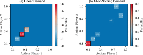
Notes. We visualize exemplary CCEs and highlight the Nash equilibria (boxes with black frames). The CCEs were computed by solving an LP where the constraints come from the definition of a CCE, and the objective was chosen such that the Wasserstein distance to the Nash equilibria is maximized; that is, we put more weight on action profiles further away from the equilibrium profiles.
For the linear demand model, the CCEs contain only actions near the NE. However, for the all-or-nothing demand model, we can find CCEs that contain dominated actions. This is why the guarantee that no-regret learners converge to a CCE is not sufficient in a Bertrand competition with all-or-nothing demand.
3.3.2. Serially Undominated Set.
Another important solution concept that can be computed by means of a simple, iterative algorithm is that of a serially undominated set. For this, let us introduce different types of dominance relationships.
(
Strongly dominated if there exists another action , such that .
Strictly dominated if there exists a mixed strategy , such that for all opponents’ action profiles .
By iterative removal of dominated actions, we end up with a serially undominated set. From Milgrom and Roberts (1990), we know that in supermodular games, the iterative procedure of removing strongly dominated strategies leads to a set where the maximum and minimum elements are component strategies of pure NE. This set includes all NE, CE, and rationalizable actions (Bernheim 1984, Pearce 1984).
Iteratively crossing out strictly dominated actions, also known as iterated strict dominance (ISD), leads to a smaller set of actions, which we will call strictly serially undominated set (SSU). A game is said to be strict dominance solvable if ISD yields a unique strategy profile. In finite games, this strategy profile is necessarily the unique NE (Fudenberg and Tirole 1991, Kolpin 2009). Note that, in order to perform ISD, we need complete information about the payoff matrix. This assumption is too strong for algorithmic pricing, which is why we will focus on bandit algorithms later. In finite games, there is a close relationship between actions that survive ISD and correlated rationalizable (CR) actions, which we will explore in the following section.
3.3.3. CR Set.
Our main convergence statement is centered on the concept of CR (Brandenburger and Dekel 1987). CR actions are actions that are a best response against any joint mixed strategy of the opponents that is also correlated rationalizable.
(
The set is called the CR.
This means that an action is in (CR) if it maximizes the player’s utility for some probability with support on . Note the recursive nature of the definition, which ensures that only actions are in the support of which are correlated rationalizable themselves.
Different from the definition of rationalizable actions (Bernheim 1984, Pearce 1984), correlated rationalizability allows the mixed strategies to be correlated probability distributions. The set of rationalizable actions is a subset of CR, but the subset relation may not be strict. Bernheim (1984) has shown that all NE are rationalizable. As a consequence, all NE are also correlated rationalizable. In finite games, ISD and correlated rationalizability give the same solution set (Levin 2006). Although this set (SSU) can be computed with ISD having the complete payoff matrix available, we will show that uncoupled mean-based algorithms also find specific instances of the CR.
3.3.4. Summary.
We summarize the relation between different solution concepts for games in Figure 2. It is well known that in finite games. The relationship between CRs (or SSD) and (C)CE is more complex. First, we can show that, similar to rationalizable actions, actions contained in the support of CE are also CR.
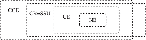
Notes. The displayed relations are between the support sets of the solution concepts. CCE, coarse correlated equilibrium; SSU, Strictly serially undominated; CR, Correlated rationalizable; CE, correlated equilibrium; NE, Nash equilibrium.
Given a finite normal-formal game, any action profile that is in the support of a CE is also in the CR.
Although it is known that CCE may contain dominated strategies (Viossat and Zapechelnyuk 2013), we can show that actions supported by a CCE are not a superset of CR actions. To show this, we use the equivalence of CR and SSU.
There exists a finite-normal form game where an action from the SSU is not in the support of any CCE.
Please refer to the Online Appendix for both proofs.
As indicated earlier, algorithms that have no (external) regret (see Equation (1)) converge to a CCE, whereas algorithms with no internal regret (such as regret matching) converge to CEs (Foster and Vohra 1997). ISD computes the SSU and thus also the CR, but this algorithm requires full access to the payoff matrix.
Table 1 summarizes properties of games that are satisfied by Bertrand competitions with different demand models (all-or-nothing, linear, and logit demand) and algorithms that are known to converge to an NE if certain of the game properties hold.
The Bertrand competition with linear demand is a potential game for which we know that even bandit algorithms such as Exp3 converge. However, other demand types do not lead to a potential game as we showed earlier. Milgrom and Roberts (1990) showed that Bertrand competition with continuous actions and linear demand is supermodular and has a unique NE, whereas with logit demand, it is log-supermodular. We do not know of convergence proofs for bandit algorithms, but we know that ISD, fictitious play, and best response dynamics find the unique NE in such supermodular games. ISD also finds correlated rationalizable sets, because they are equivalent to serially undominated sets. Our main analytical contribution is to show that mean-based algorithms, with Exp3 as the leading example, converge to the correlated rationalizable set. Importantly, in a Bertrand competition with all-or-nothing or linear demand, this set is either a singleton, meaning it must be the NE, or consists of only two adjacent actions.
4. Convergence of Mean-Based Algorithms
Let us now focus on mean-based algorithms. These are online optimization algorithms that pick actions with low average rewards with low probability (Braverman et al. 2018, Deng et al. 2022).
(
There are many no-regret algorithms, such as Exp3, multiplicative weights, and the FTPL algorithm, which are also mean based. We know from Kolumbus and Nisan (2022) that if a mean-based algorithm converges to a CCE, then the CCE is co-undominated, which avoids outcomes with dominated strategies as illustrated in Figure 1(b). Deng et al., 2022 and Feng et al. (2021) analyzed the convergence of mean-based algorithms in first-price and second-price auctions, and they found convergence in the complete-information games. We focus on Bertrand competitions, which are different due to the various demand models. In what follows, we provide proof that mean-based algorithms converge to strategy profiles in the correlated rationalizable set.
We analyze convergence in a time-average and in a last-iterate sense (Anagnostides et al. 2023). Although the former measures the fraction of times that all players have chosen actions according to a reference profile or reference set of actions, the latter makes a statement about the current strategy of the players, that is, their current distribution over action selections.
(
With this definition at hand, we can state our central convergence theorem. For brevity of notation, we restrict ourselves to an informal formulation and provide a mathematically thorough version in Section A.4.8 of the Online Appendix. The proof, building on techniques introduced by Feng et al. (2021) and Deng et al., 2022, is provided in Section A.4 of the Online Appendix.
(
Thus far, we have shown that players will eventually play CR actions in almost every round. But we can also say something about the actual (mixed) strategy profile of the players, that is, about last-iterate convergence. In the general setting of the previous theorem, we can only show that the support of the mixed strategies is within the CR actions in the limit. In the special case, where the CR actions correspond to the unique NE, for example, in the all-or-nothing demand setting as described in Proposition 9, we get last-iterate convergence to the NE. We formalize this result in the corollary below and provide its proof in Section A.4.9 of the Online Appendix.
In games with a unique pure NE being the only correlated rationalizable action, mean-based algorithms converge almost surely to the NE in last-iterate, that is, , where is the sequence of mixed strategy profiles and .
Our analysis leads to a corollary that is of independent interest and beyond the analysis of Bertrand competition.
Mean-based algorithms converge to strategy profiles in the serially undominated set.
This follows from the fact that serially undominated sets are equivalent to CR sets of strategy profiles. Next, we focus on the class of Bertrand competition games. Let us present our second main result informally.
Informal Theorem. In symmetric Bertrand competition games with standard or linear demand and discrete actions, mean-based algorithms converge almost surely to actions that are close to their NE.
For this, we just need to show that the CR sets are close to the set of NE for the two demand models, which we do in Section A.3 of the Online Appendix.
5. Experimental Analysis
In our experimental analysis, we analyze the behavior of various bandit algorithms in Bertrand oligopolies with different demand models. The focus variables of our experiments are the converged prices and the convergence behavior. We focus on scenarios that our theoretical contribution does not cover. We use algorithms that are well known but (with the exception of Exp3) not known to be mean based, and we simulate their behavior in a variety of Bertrand oligopolies.
In our numerical experiments, most algorithms consistently reach NE prices within a few iterations, indicating that even without tens of thousands of repeated interactions and without the mean-based property, supra-competitive prices are rarely established. By including different demand functions and both symmetric and asymmetric environments, we show that our findings are robust across a wide range of treatments.
5.1. Selected Algorithms
In our study, we include -greedy, UCB, Thompson sampling, and Exp3, which are widely used and cited in the literature (Bubeck, 2011). All bandit algorithms share similarities. First, an action is selected according to some potentially random action-selection rule that is based on past experiences. Then, the agent receives a corresponding reward feedback with which it subsequently updates its internal state. We describe this generic scheme in Algorithm 1. All algorithms that we analyze follow this generic scheme while implementing distinct rules for selecting actions and updating their beliefs. Details of the algorithms can be found in Section B.1 of the Online Appendix. Typically, the algorithms allow for different variations, and each description describes a family of algorithms.
(
Initialization: Algorithm parameters
for do
get_action(, t) // Agents choose action.
environment() // Agents submit actions and observe own utility.
update(, , , t) // Agents update their strategy.
end for
5.2. Experiment Setup
We demonstrate that even in treatments where no analytical convergence results are available, convergence to competitive prices can be observed consistently with many bandit algorithms. Supra-competitive (“collusive”) prices, which are prices between the NE and the joint profit-maximizing prices, only occur under symmetric combinations of certain algorithms. We characterize supra-competitive prices via the following metrics. Let be the largest component strategies of any pure NE and let be the actions played in the monopoly. We define the price-competition index of player i by
A price-competition index of zero captures that player i plays , and thus is competitive. A value of one means that the agent plays indicates cooperative pricing. The profit-competition index represents the fraction of monopolistic payoff surplus that all agents could achieve in total.
Let us briefly discuss the choice of metrics. In essence, we want to capture a deviation from competitive play (NE) to cooperation. A NE naturally lends itself as the lower bound of our metric’s values, but the choice of the upper deserves discussion. As noted by Loots and den Boer (2023), multiple notions of collusive prices are reasonable, and joint profit maximization might not always be the adequate choice. In line with previous research (Calvano et al. 2020a), we nonetheless select these prices as our upper reference points, because in our analyzed settings, joint profit maximization is beneficial to all firms. Being a joint maximum, it is Pareto-optimal for sellers, too. As indicated by Loots and den Boer (2023), joint profit maximization also exhibits the highest price increase and the worst effect on consumer welfare, on average.
In the following, we introduce the treatment variables of our experiments, such as the oligopoly configurations and the bandit algorithms, as well as the experiment setup. We then state the conclusions drawn from our experiments and present the empirical evidence supporting them. In our experiments, we vary the games that the agents compete in, the algorithms they use, and the number of competitors they face. An experiment is formed by a unique combination of these factors. Table 2 provides an overview of the treatment and focus variables.
|
Table 2. Treatment and Focus Variables of the Experiments
| Treatment variables | Variations |
|---|---|
| Oligopoly model | Demand models (standard, linear, logit), symmetric/asymmetric parameterization |
| Algorithms | UCB-T, Exp3-, -Greedy, TS, (UCB1, Q-Learning, MWU) |
| Number of competitors | 2–10 |
| Focus variables | Description |
|---|---|
| Prices | Prices after convergence |
| Convergence speed | Time to convergence and convergence behavior |
5.2.1. Oligopoly Model.
Our oligopolies model the demand and the costs that firms face. They are based on the games described in Section 3.2. We implemented models with standard, linear, and logit demand functions. Depending on the parameter choices, the utility functions are the same for all agents (symmetric game) or not (asymmetric game). Our experiments are based on the following instances of Bertrand competition. The first three configurations are symmetric games with standard demand (O1), linear demand (O2), and logit demand (O3). O2 and O3 are inspired by Calvano et al. (2020a) and Hansen et al. (2021), respectively. Likewise, we defined asymmetric counterparts for duopolies with linear demand (O2′) and logit demand (O3′). The asymmetric settings are a step toward more realistic scenarios where firms might face different costs and demand structures. The configurations are summarized in Table 3. We selected price ranges that span the NE prices and joint-profit-maximizing prices, including a small margin. The agents can choose from 21 evenly distributed prices within this range. For example, an agent in O3 can select actions from the set . Other discretizations, and in particular asymmetric discretizations for the players, did not substantially change our results in preliminary experiments.
|
Table 3. Parameterization of the Bertrand Oligopoly Models
| Model | Demand | Costs | Other parameters | Price range | Nash | Monopoly |
|---|---|---|---|---|---|---|
| O1 | Standard | — | [0.05, 1.00] | |||
| O2 | Linear | , , | [0.00, 1.00] | |||
| O3 | Logit | , , | [1.00, 2.00] | |||
| O2′ | Linear | , , | [0.00, 1.00] | |||
| O3′ | Logit | , , , | [1.00, 2.00] |
Notes. The (pure) Nash equilibria and monopoly prices are stated for the discretized game. In case of multiple equilibria, the maximum prices are taken.
5.2.2. Algorithms.
We investigate the behavior of four widespread bandit algorithms. First, we evaluate a variant of the UCB-tuned (UCB-T) algorithm that resolves ties randomly and does not eliminate actions. Next, we run experiments with the simple -greedy algorithm (-Greedy) and an Exp3 (Exp3- ) algorithm with fixed exploration rate . We note that this version of Exp3 is not mean based. Known mean-based versions of Exp3 suffer from a very slowly decaying exploration rate, which makes them impractical for experiments and applications. Finally, we implemented an algorithm (TS) that performs Thompson sampling with Gaussian priors, likelihoods, and posteriors. We note that our experiment results are stable against reasonable modifications of the parameters. In one result on mean-based algorithms, we also analyze MWU and the mean-based version of Exp3 introduced by Braverman et al., 2018. In the Online Appendix, we also report results on Q-learning to provide a comparison. However, given the multitude of hyperparameters available in this algorithm, we restrict our analysis to a few experiments replicating prior results. We also compare these results to those of the algorithms in the main part of the article.
5.2.3. Number of Competitors.
Some of our empirical results are based on the number of firms that compete in an oligopoly. The symmetric games (O1, O2, O3) can be easily extended to an arbitrary number of players. We investigate numbers between 2 and 10 for an oligopoly based on O2.
We run each experiment 10 times with random seeds from zero to nine. Fixing the seeds allows us to reproduce results despite the random nature of the algorithms. Each run consists of 250,000 iteration steps during which the agents first submit their actions simultaneously and independently to the market. Then, the demands are evaluated, and the agents observe their respective rewards. The agents update their beliefs at the end of each step. We found that almost all our experiments converged within the provided time frame.
5.3. Results
Let us now report the main results of our experimental analysis.
5.3.1. Convergence Speed with Mean-Based Algorithms.
We first focus on markets with mean-based algorithms. Our convergence guarantee applies, but the speed of convergence is unknown. We consider the mean-based versions of MWU and Exp3 that have been described by Braverman et al., 2018. Figure 3 shows the evolution of the price-competition index over the course of the experiments. We observe convergence to very low index values. Although the MWU algorithm reaches the final outcome within a few iterations, the Exp3 algorithm requires noticeably more iterations. This is expected because MWU has access to full feedback, whereas Exp3 only receives bandit feedback. Below, we use a different version of Exp3 that is faster than its mean-based counterpart.
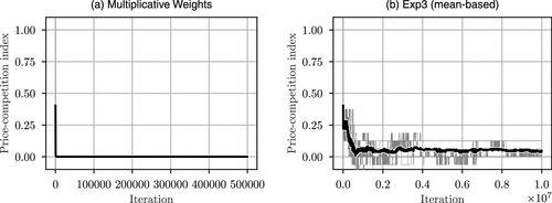
Notes. The experiments are based on the symmetric environment with linear demand (O2). The figures display the competition indices based on the charged prices (running medians over 1,000 steps) for 10 runs of the experiment in thin lines. The thick line shows the average of all runs and thus indicates the overall trend.
5.3.2. Algorithmic Pricing in Duopolies.
Next, we analyze duopolies with different algorithms that are not mean based anymore. We first report the prices at the end of the experiments in two-player games. In Section B.2 of the Online Appendix, we provide an analysis of the convergence speed: After 250,000 iterations, the algorithms consistently settle at a price level, so we can assume convergence. Our first result makes a statement about the price levels agents eventually reach.
Supra-competitive pricing only evolves with UCB algorithms under self-play. Other algorithms consistently price close to the NE prices. In particular, combinations of diverse algorithms rarely display noncompetitive behavior. This happens for all demand models (standard, linear, logit) and for symmetric and asymmetric settings.
We visualize these results in Figure 4, which displays the profit- and price-competition indices found in our experiments. We average the indices over settings, runs, and—if applicable—over agents. In settings with two identical competing algorithms (diagonal entries), we only observe noncompetitive behavior with the UCB-T algorithm. In this case, prices and profits are high, meaning that cooperating algorithms indeed benefit from their noncompetitive play. The combined settings of any two different algorithms show competition indices close to zero, with a combination of UCB-T and -Greedy resulting in only slightly supra-competitive prices.
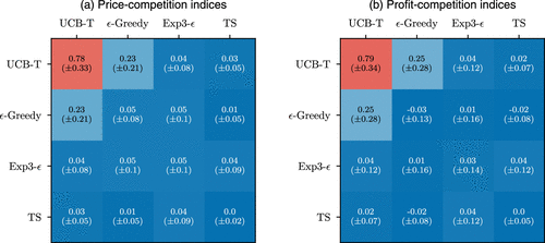
Notes. We visualize the competition indices based on (a) the median prices and (b) the mean profits in the last 1,000 steps of several combinations of algorithms. The displayed numbers are the numeric values of the competition indices; the values in brackets display their corresponding standard deviation. Averages and standard deviations were computed over two agents, 10 runs, and the five settings O1–O3′.
Our experiments also demonstrate that noncompetitive behavior with Bandit algorithms does not develop in a stable manner. Although we could observe high prices with UCB-T for all demand functions, and in symmetric as well as asymmetric games, these experiments usually suffer from a high variance between runs, making the result unpredictable in advance. In contrast, competitive algorithms performed consistently in all environments and all runs.
Although experiments with two players in simplified oligopolies are useful to extract the essence of algorithmic interaction, we also investigated extensions of our games with more players and richer demand functions. We provide our results in Online Appendix B.
6. Conclusions
The discussion of algorithmic collusion is largely based on the experimental results of specific algorithms and versions of the Bertrand competition. In general, learning algorithms do not converge to an equilibrium. However, we prove that important algorithms do so in repeated Bertrand pricing competition with all-or-nothing and linear demand models. The convergence of mean-based algorithms to correlated rationalizable strategies is of independent interest and might be useful for the analysis of different games as well. The result closes a gap in the literature on learning in games, which largely focused on algorithms with no internal or external regret, which converge to correlated or coarse correlated equilibria, respectively. Mean-based algorithms such as Exp3 only require bandit feedback after each round, a realistic assumption for algorithms used in algorithmic pricing. The fact that correlated rationalizable strategy profiles coincide with the set of Nash equilibria in Bertrand competition games is an important insight, and it shows that such games can be learned even with very simple algorithms relevant in practice.
We also show experimentally that when (not mean-based) online optimization algorithms are used in combination, supra-competitive prices are mostly not sustained in experiments. If sellers use UCB or Q-learning symmetrically, they might learn prices higher than the NE. A combination of different algorithms, however, rarely develops noncompetitive outcomes. Such insights are important for regulators when they want to identify noncompetitive behavior in online markets. Although multiarmed bandit algorithms are an important and widely used class of algorithms used for algorithmic pricing, one cannot guarantee that sellers don’t use other algorithms. In future research, it will be valuable to analyze and classify alternative algorithms and models. The properties that we showed for the Bertrand competition will also be useful for subsequent studies.
1 See https://www.businessinsider.com/amazon-price-changes-2018-8.
2 See https://towardsdatascience.com/dynamic-pricing-with-multi-armed-bandit-learning-by-doing-3e4550ed02ac, https://www.griddynamics.com/blog/dynamic-pricing-algorithms.
3 Note that by the Folk theorem, such a supracompetitive price could still be an equilibrium in an infinitely repeated game if players have sufficient patience (Fudenberg and Tirole 1991).
4 Note that in this literature review, we focus on algorithms that were not designed to collude (Meylahn and den Boer 2022).
References
- (2023) Artificial intelligence: Can seemingly collusive outcomes be avoided? Management Sci. 69(9):5042–5065.Link, Google Scholar
- (2024a) Collusion by mistake: Does algorithmic sophistication drive supra-competitive profits? Eur. J. Oper. Res. 318(3):927–953.Crossref, Google Scholar
- (2024b) Algorithmic collusion: Where are we and where should we be going? Preprint, submitted August 7, https://doi.org/10.2139/ssrn.4891033.Google Scholar
- AB-325 Cartwright Act: Violations. California Legislative Information, https://leginfo.legislature.ca.gov/faces/billNavClient.xhtml?bill_id=202520260AB325.Google Scholar
- (2023) On the convergence of no-regret learning dynamics in time-varying games
. Adv. Neural Inform. Processing Systems, vol. 36 (Curran Associates Inc., Red Hook, NY), 16367–16405.Crossref, Google Scholar - (2024) The impact of artificial intelligence design on pricing. J. Econom. Management Strategy 33(2):276–304.Crossref, Google Scholar
- (2002) The nonstochastic multiarmed bandit problem. SIAM J. Comput. 32(1):48–77.Crossref, Google Scholar
- (1995) Gambling in a rigged casino: The adversarial multi-armed bandit problem. Proc. IEEE 36th Annual Foundations Comput. Sci. (IEEE Computer Society, Washington, DC).Google Scholar
- (1987) Correlated equilibrium as an expression of Bayesian rationality. Econometrica 55(1):1–18. Crossref, Google Scholar
- Bailey JP, Piliouras G (2018) Multiplicative weights update in zero-sum games. Tardos E, Elkind E, Vohra R, eds. Proc. 2018 ACM Conf. Econom. Comput. (ACM, New York).Google Scholar
Ballard D, Costello K, Lo M, Scarborough M (2025) California looks to crack down on algorithmic pricing and clarify antitrust pleading standards. JD Supra, https://www.jdsupra.com/legalnews/california-looks-to-crack-down-on-3793901/.Google Scholar- (2018) Optimal pricing in e-commerce based on sparse and noisy data. Decision Support Systems 106:53–63.Crossref, Google Scholar
- (1984) Rationalizable strategic behavior. Econometrica 52(4):1007–1028.Crossref, Google Scholar
- (1883a) Review of “Theorie mathematique de la richesse sociale” and of “Recherches sur les principles mathematiques de la theorie des richesses. J. De Savants 67:499.Google Scholar
- (1883b) Théorie mathématique de la richesse sociale. J. Des Savants 67(1883):499–508.Google Scholar
- Computing Bayes–Nash equilibrium strategies in auction games via simultaneous online dual averaging. Oper. Res. 73(2):1102–1127.Link, Google Scholar
- (1987) Rationalizability and correlated equilibria. Econometrica 55(6):1391–1402.Crossref, Google Scholar
Braverman M, Mao J, Schneider J, Weinberg M (2018) Selling to a no-regret buyer. Tardos E, Elkind E, Vohra R, eds. Proc. 2018 ACM Conf. Econom. Comput. (Association for Computing Machinery, New York) .Google Scholar- (1951) Iterative solution of games by fictitious play. Activity Anal. Production Allocation 13(1):374–376.Google Scholar
- (2023) Competition in pricing algorithms. Amer. Econom. J. Microeconom. 15(2):109–156.Crossref, Google Scholar
- . Lecture notes, Princeton University, Princeton, NJ. Google Scholar
- (2021b) Algorithmic collusion with imperfect monitoring. Internat. J. Indust. Organ. 79:102712.Crossref, Google Scholar
- (2019) Algorithmic pricing what implications for competition policy? Rev. Industrial Organ. 55(1):155–171.Crossref, Google Scholar
- (2020a) Artificial intelligence, algorithmic pricing, and collusion. Amer. Econom. Rev. 110(10):3267–3297.Crossref, Google Scholar
- Algorithmic Collusion, Genuine and Spurious. Social Science Research Network.Google Scholar
Calzolari G, Hanspach P (2024) Pricing algorithms out of the box: A study of the repricing industry. Preprint, submitted July 1, http://dx.doi.org/10.2139/ssrn.4871394.Google Scholar- (2020b) Protecting consumers from collusive prices due to AI. Science (1979) 370(6520):1040–1042.Google Scholar
- (2006) Prediction, Learning, and Games (Cambridge University Press, Cambridge, UK).Crossref, Google Scholar
Chen L, Mislove A, Wilson C (2011) An empirical analysis of algorithmic pricing on Amazon marketplace. Bourdeau J, Hendler JA, Nkambou Nkambou R, Horrocks I, Zhao BY, eds. Proc. 25th Internat. Conf. World Wide Web (International World Wide Web Conferences Steering Committee, Geneva, CHE) .Google Scholar- (2025) PyBLP.Google Scholar
- (1838) Recherches Sur Les Principes Mathématiques De La Théorie Des Richesses (L. Hachette).Google Scholar
- (2009) The complexity of computing a Nash equilibrium. SIAM J. Comput. 39(1):195–259.Crossref, Google Scholar
- (2015) Dynamic pricing and learning: Historical origins, current research, and new directions. Surveys Oper. Res. Management Sci. 20(1):1–18.Crossref, Google Scholar
den Boer AV (2023) Algorithmic collusion: A mathematical definition and research agenda for the OR/MS community. Preprint, submitted November 7 , https://dx.doi.org/10.2139/ssrn.5012923.Google Scholarden Boer AV, Meylahn JM, Schinkel MP (2024) Artificial collusion: Examining supracompetitive pricing by Q-learning algorithms. Preprint, submitted September 13, http://dx.doi.org/10.2139/ssrn.4213600.Google ScholarDeng S, Schiffer M, Bichler M (2024) On the existence of algorithmic collusion in dynamic pricing with deep reinforcement learning. Flath CM, Gust G, Thiesse F, Winkelmann A, eds. Wirtschaftsinformatik 2024 Proc. (Association for Information Systems (AIS), Atlanta) .Google ScholarDeng X, Hu X, Lin T, Zheng W (2022) Nash convergence of mean-based learning algorithms in first price auctions. Laforest F, Troncy R, Simperl E, Agarwal D, Gionis A, Herman I, Médini L, eds. Proc. ACM Web Conf. 2022 (Association for Computing Machinery, New York) .Google ScholarDouglas C, Provost F, Sundararajan A (2024) Naive algorithmic collusion: When do bandit learners cooperate and when do they compete? Susarla A, Chau M, Hinz O, eds. ICIS 2024 Proc. (Association for Information Systems (AIS), Atlanta) .Google Scholar- (2021) Novel pricing strategies for revenue maximization and demand learning using an exploration–exploitation framework. Soft Comput. 25(17):11711–11733.Crossref, Google Scholar
- (2022) Robust algorithmic collusion. Preprint, submitted January 2, https://arxiv.org/abs/2201.00345.Google Scholar
- (2021) Convergence analysis of no-regret bidding algorithms in repeated auctions. Proc. AAAI Conf. Artificial Intelligence 35(6):5399–5406.Crossref, Google Scholar
- (1997) Calibrated learning and correlated equilibrium. Games Econ. Behav. 21(1):40–55.Crossref, Google Scholar
- (1999) Regret in the on-line decision problem. Games Econom. Behav. 29(1):7–35.Crossref, Google Scholar
- (1999)
The Theory of Learning in Games , MIT Press Series on Economic Learning and Social Evolution, 2nd ed., vol. 2 (MIT Press, Cambridge, MA).Google Scholar - (1991) Game Theory (MIT Press, Cambridge, MA).Google Scholar
- (2023) Learning to price under competition for multinomial logit demand. Preprint, submitted October 10, https://doi.org/10.2139/ssrn.4572453.Google Scholar
- (2021) Frontiers: Algorithmic collusion: Supra-competitive prices via independent algorithms. Marketing Sci. 40(1):1–12.Link, Google Scholar
- (2018) Developing competition law for collusion by autonomous artificial agents. J. Competition Law Econom. 14(3):331–363.Crossref, Google Scholar
- (2003) Uncoupled dynamics do not lead to Nash equilibrium. Amer. Econom. Rev. 93(5):1830–1836.Crossref, Google Scholar
- (2006) Stochastic uncoupled dynamics and Nash equilibrium. Games Econom. Behav. 57(2):286–303.Crossref, Google Scholar
Hartline J (2026) Clarification of ‘Algorithmic collusion without threats’. Preprint, submitted February 15, https://arxiv.org/abs/2602.22232.Google ScholarHartline JD, Long S, Zhang C (2024) Regulation of algorithmic collusion. Weitzner DJ, Yoo CS, Canetti R, eds. Proc. 2024 Sympos. Comput. Sci. Law (Association for Computing Machinery, New York) .Google Scholar- (2017) Learning with bandit feedback in potential games. Adv. Neural Inform. Processing Systems, vol. 30 (Curran Associates Inc., Red Hook, NY).Google Scholar
- (2015) Correlated equilibria in homogeneous good Bertrand competition. J. Math. Econom. 57:31–37.Crossref, Google Scholar
- (2024) V-Learning—A simple, efficient, decentralized algorithm for multiagent reinforcement learning. Math. Oper. Res. 49(4):2295–2322.Link, Google Scholar
- (2023) Platform design when sellers use pricing algorithms. Econometrica 91(5):1841–1879.Crossref, Google Scholar
- (2022) Dynamic pricing under competition using reinforcement learning. J. Revenue Pricing Management 21(1):50–63.Crossref, Google Scholar
- (2021) Autonomous algorithmic collusion: Q-learning under sequential pricing. RAND J. Econom. 52(3):538–558.Crossref, Google Scholar
- (2009) Strict dominance solvability without equilibrium. Econom. Bull. 29(1):51–55. Google Scholar
Kolumbus Y, Nisan N (2022) Auctions between regret-minimizing agents. Laforest F, Troncy R, Simperl E, Agarwal D, Gionis A, Herman I, Médini L, eds. Proc. ACM Web Conf. 2022 (Association for Computing Machinery, New York) .Google Scholar- (2024) Less than meets the eye: Simultaneous experiments as a source of algorithmic seeming collusion. Preprint, submitted July 5, https://doi.org/10.2139/ssrn.4498926.Google Scholar
- (2006) Solution concepts. Notes. https://web.stanford.edu/∼jdlevin/Econ%20286/Solution%20Concepts.pdf.Google Scholar
- (2023) Data‐driven collusion and competition in a pricing duopoly with multinomial logit demand. Production Oper. Management 32(4):1169–1186.Crossref, Google Scholar
- (2019) Learning in games with continuous action sets and unknown payoff functions. Math. Programming 173(1–2):465–507.Crossref, Google Scholar
- (2024) A unified stochastic approximation framework for learning in games. Math. Programming 203(1):559–609.Crossref, Google Scholar
- (2018) Cycles in adversarial regularized learning. Proc. 29th Ann. ACM-SIAM Sympos. Discrete Algorithms (SIAM, Philadelphia), 2703–2717.Google Scholar
- (2022) Learning to collude in a pricing duopoly. Manufacturing Service Oper. Management 24(5):2577–2594.Link, Google Scholar
- (1990) Rationalizability, learning, and equilibrium in games with strategic complementarities. Econometrica 1255–1277.Crossref, Google Scholar
- (1991) Adaptive and sophisticated learning in normal form games. Games Econom. Behav. 3(1):82–100.Crossref, Google Scholar
- (2022) Nash, conley, and computation: Impossibility and incompleteness in game dynamics. Preprint, submitted March 26, https://arxiv.org/abs/2203.14129.Google Scholar
- (1996) Potential games. Games Econom. Behav. 14(1):124–143.Crossref, Google Scholar
- (2019) Low-rank bandit methods for high-dimensional dynamic pricing. Adv. Neural Inform. Processing Systems, vol. 32 (Curran Associates Inc., Red Hook, NY).Google Scholar
OECD (2017) Algorithms and collusion: Competition policy in the digital age. Technical report, OECD, Paris.Google Scholar- (2017)
Multiplicative weights update with constant step-size in congestion games: Convergence, limit cycles and chaos . Guyon I, Luxburg UV, Bengio S, Wallach H, Fergus R, Vishwanathan S, Garnett R, eds. Adv. Neural Inform. Processing Systems, vol. 30 (Curran Associates Inc., Red Hook, NY).Google Scholar - (1984) Rationalizable strategic behavior and the problem of perfection. Econometrica 52(4):1029–1050.Crossref, Google Scholar
- (2024) Survey of dynamic pricing based on Multi-Armed Bandit algorithms. ACE 37(1):160–165. Crossref, Google Scholar
- (2014) Real-time dynamic pricing in a non-stationary environment using model-free reinforcement learning. Omega 47:116–126.Crossref, Google Scholar
- (1974) A two-armed bandit theory of market pricing. J. Econom. Theory 9(2):185–202.Crossref, Google Scholar
- (2018) The prevalence of chaotic dynamics in games with many players. Sci. Rep. 8(1):1–13.Crossref, Google Scholar
- (2010) Population Games and Evolutionary Dynamics. Economic Learning and Social Evolution (MIT Press, Cambridge, MA).Google Scholar
- (2022) On the emergence of cooperation in the repeated prisoner’s dilemma. Preprint, submitted November 24, https://arxiv.org/abs/2211.15331.Google Scholar
- (2011) Online learning and online convex optimization. Foundations Trends Machine Learn. 4(2):107–194.Crossref, Google Scholar
- (1964) Some topics in two-person games. Adv. Game Theory 52:1–29. Google Scholar
- (2018) On best-response dynamics in potential games. SIAM J. Control Optim. 56(4):2734–2767.Crossref, Google Scholar
- Multi-armed bandit algorithms for cournot games. Research Square, https://www.researchsquare.com/article/rs-2928787/v1.Google Scholar
- (1979) Equilibrium points in nonzero-sum n-person submodular games. SIAM J. Control Optim. 17(6):773–787.Crossref, Google Scholar
- (1998) Supermodularity and Complementarity (Princeton University Press, Princeton, NJ).Crossref, Google Scholar
Trovo F, Paladino S, Restelli M, Gatti N (2015) Multi-armed bandit for pricing. Proc. 12th Eur. Workshop Reinforcement Learn .Google Scholar- (2013) No-regret dynamics and fictitious play. J. Econom. Theory 148(2):825–842.Crossref, Google Scholar
- (2001) Oligopoly Pricing: Old Ideas and New Tools (MIT Press, Cambridge, MA).Google Scholar
- (2020) No-regret learning and mixed Nash equilibria: They do not mix. Adv. Neural Inform. Processing Systems, vol. 33 (Curran Associates Inc., Red Hook, NY), 1380–1391. Google Scholar
- (2008) Learning agents in a Cournot oligopoly model. J. Econom. Dynamic Control 32(10):3275–3293.Crossref, Google Scholar
- (2022) Learning rationalizable equilibria in multiplayer games. Preprint, submitted October 20, https://arxiv.org/abs/2210.11402.Google Scholar
- (2008)
Correlated equilibrium of bertrand competition . Papadimitriou C, Zhang S, eds. Internet and Network Economics (Springer, Berlin, Heidelberg), 166–177.Crossref, Google Scholar - (2024) Competitive demand learning: A noncooperative pricing algorithm with coordinated price experimentation. Production Oper. Management 33(1):48–68. Google Scholar
- (2010) Strategic Learning and Its Limits (Oxford University Press, Oxford, UK).Google Scholar

