
Systematic Differences and Random Rates: Reconciling Gibrat’s Law with Firm Differences
Abstract
A fundamental premise of the strategy field is the existence of persistent firm-level differences in resources and capabilities. This property of heterogeneity should express itself in a variety of empirical “signatures,” such as firm performance and arguably systematic and persistent differences in firm-level growth rates, with low cost firms outpacing high cost firms. While this property of performance differences is a robust regularity, the empirical evidence on firm growth and Gibrat’s law does not support the later conjecture. Gibrat’s law, or the “law of proportionate effect,” states that, across a population of firms and over time, firm growth at any point is, on average, proportionate to size of the firm. We develop a theoretical argument that provides a reconciliation of this apparent paradox. The model implies that in early stages of an industry history. firm growth may have a systematic component, but for much of an industry’s and firm’s history should have a random pattern consistent with the Gibrat property. The intuition is as follows. In a Cournot equilibrium, firms of better “type” (i.e., lower cost) realize a larger market share, but act with some restraint on their choice of quantity in the face of a downward sloping demand curve and recognition of their impact on the market price. If firms are subject to random firm-specific shocks, then in this equilibrium setting a population of such firms would generate a pattern of growth consistent with Gibrat’s law. However, if broader evolutionary dynamics of firm entry, and the subsequent consolidation of market share and industry shake-out is considered, then during early epochs of industry evolution, one would tend to observe systematic differences in growth rates associated with firm’s competitive fitness. Thus, it is only in these settings far from industry equilibrium that we should see systematic deviations from Gibrat’s law.
It is conventional to speak of “stylized facts” about economic activity. The aim of identifying these regularities is to both inform our understanding of the world and provide a basis for our theorizing about the world. In the industrial organization literature, two of the most prominent regularities are Gibrat’s (1931) law of random proportionate growth rates and the presence of systematic firm differences in firm capabilities and their broader performance. As Geroski (2000) has noted, these two properties seem strikingly in conflict.1 If there exists pronounced and persistent firm differences in their capabilities or, more broadly, in their economic value proposition (allowing for differences in value creation, as well as cost differences), why aren’t those differences expressed in differential growth rates? We reconcile this apparent conflict by contrasting the pattern of growth rates in a competitive equilibrium with the realized patterns in route to this equilibrium outcome.
A well-known and broadly accepted fact in the empirical strategy literature is the existence of persistent firm-level differences in resources and capabilities, which in turn translate into firm-level differences in costs, value creation, and ultimately profitability (Schmalensee 1985, Rumelt 1991, McGahan and Porter 1997). One might also expect to see these firm differences expressed in the form of systematic and persistent differences in firm-level growth rates, with low cost firms outpacing high cost firms. However, the empirical evidence on firm growth and Gibrat’s law does not support this conjecture. Gibrat’s law, or the “law of proportionate effect,” states that, across a population of firms and over time, firm growth at any point is, on average, proportionate to a firm’ size, i.e., firm growth rates are scale-invariant and independent of initial size. Apparently, persistent differences in firm capabilities are not expressed in firm growth rates.
In the empirical literature on firm growth (Ijiri and Simon 1967, Axtell 2001, Coad 2009), size is typically measured by sales, although other indicators, such as number of employees, have been explored. Estimation of growth rates allows for random factors by assuming that firm size evolves from period to period as a random walk in the logarithm of sales, with i.i.d. shocks.2 This very strong and simple assumption has a number of implications, one of which is that the firm size distribution is log normal, with ever increasing variance of the logs. While the Gibrat process is quite stark in its simple but bold claim, its descriptive accuracy is quite high (Geroski 2000, Axtell 2001, Coad 2009). As a result, researchers have tended to take it as a baseline and taken up the tasks of analyzing deviations from it, both in the period-to-period firm-level dynamics and in the long run distribution of firm size (Evans 1987, Bottazzi and Secchi 2006).
Thus, models in this tradition have a dual grounding in empirical regularities. First, the characterization of the stochastic dynamics at the firm level should roughly capture some stylized facts about real change processes. Second, the asymptotic firm size distribution implied by the model should correspond with empirical observations of these cross sections. An important and classic example of this dual approach is the work of Ijiri and Simon (1964 and 1967), whose process model combines growth of existing firms where the property of “proportionate effect” is assumed to hold, and the characterization of the industry dynamics includes the entry by new firms at a designated minimum scale. The process leads asymptotically to a Pareto distribution. A special case, in which the probability of sizes in the upper tail of the size distribution greater than a value s is inversely proportional to the value s, is known as Zipf’s law (Axtell 2001).
While the Ijiri and Simon approach provides a useful baseline model that is broadly consistent with the basic empirical regularities of firm growth rates and firm size distribution, there are other important lines of inquiry that have supplemented this work. Jovanovic (1982) develops a model of a firm learning about its “type,” where type is characterized by its cost value. In this set-up, firms analyze their output and possible exit decision based on their assessment of their cost value, which itself is subject to stochastic shocks. Building on this work, Hopenhayn (1992) considers the implications for the aggregate pattern of turnover, entry and exit, in a steady-state equilibrium model. While these models bring in useful explicit firm-level calculus regarding output and exit decisions, the models themselves are premised on an industry structure of a continuum of firms, each arbitrarily small so as to be treated as price-takers in market competition. As a consequence, this line of work cannot speak to the empirical patterns of industry evolution of phases of net growth in the number of firms, a period of “shakeout” or decline, and a subsequent period of relative stability (Gort and Klepper 1982). Klepper (1996) provides an account of these patterns based on the logic of firm size impacting its investment in process innovations, leading to later and smaller industry entrants being driven from the market. Klepper’s work is targeted at this pattern over an industry lifecycle of entry, exit, and aggregate industry size, but the issue of firm growth rates is not developed. In another line of work, both Sutton (1997) and Klepper and Thompson (2006) use the random arrival of new “sub-markets” to explain firm growth rates, but these analyses do not link back to the consideration of the pattern of entry and exit of an industry’s lifecycle.
We develop a relatively simple model that, while not fully general, is able to capture both issues of firm growth rates and industry evolution. Further, this joint consideration provides a theoretical reconciliation of evidence that suggests firm growth is, at the same time, both systematic and random. The intuition is as follows. In a Cournot equilibrium, firms of better “type” (i.e., lower cost) realize a larger market share, but act with some restraint on their choice of quantity in the face of a downward sloping demand curve and recognition of their impact on the market price. If firms are subject to random firm-specific shocks, then in this equilibrium setting a population of such firms would generate a pattern of growth consistent with Gibrat’s law. However, if broader evolutionary dynamics of firm entry, and the subsequent consolidation of market share and industry shake-out are considered (Klepper 1996), then during early epochs of industry evolution one would tend to observe systematic differences in growth rates associated with firms’ competitive fitness. Thus, it is only in these settings far from industry equilibrium that we should see deviations from Gibrat’s law. In the Model Structure section, we lay out the structure of our formal model for which we provide computational results in the Results section.
Model Structure
We develop a fairly conventional model of Cournot competition, but one that incorporates the entry and exit dynamics of realized and potential competitors (Klepper 1996, Knudsen et al. 2014). As is typical in such models, the demand environment is treated as being fixed. We represent market demand by an exponential function, where
In each period, there is a cohort of Nc potential entrants where Nc is fixed to a constant value. Potential entrants randomly draw a firm-specific cost value ci. By cost values, we refer to unit costs of individual firms. Cost values are drawn from the general beta distribution with shape parameters (α, β) and support in a non-negative finite interval. Since cost distributions determine the arrival rate of firms entering with low versus high cost values, this distribution has significant influence on the realized firm and industry dynamics as well as steady state properties. In our baseline model, we examine the effect of a Bell-shaped cost distribution with α = 5 and β = 5.
Cost values may be subject to random firm-specific shocks. That is, stochastic variation can perturb firm-specific cost values ci so that the next period’s cost value ci, t + 1 is given by
Scale Adjustment
A firm calculates its desired scale of production q* based on its own unit cost and the cost values of all firms that are currently operating. As a result, the desired scale of production q* is a moving target that the firm aims to achieve by expanding (or reducing) its current production capacity. The realized scale of a given firm’s production at period t + 1 is modeled as
We find the optimal output by analytically solving for the Cournot equilibrium output.4 For the exponential case, the elasticity of demand is Q1/Q, and the Cournot equilibrium output for firm i is
Firms remain in the market as long as their unit cost ci is less than industry price P. These firms are found sequentially by starting with the highest cost firm and eliminating it, then recomputing the industry equilibrium in the absence of this highest cost firm. This process is continued until all the remaining firms are viable. The target output of each firm depends on its unit cost:
Serial Correlation in the Rate of Growth
Serial correlation is a central measure since we are interested in examining the seeming paradox noted by Geroski (2000), where apparently random variation in firm growth rates is associated with persistent heterogeneity in firm attributes. If there is no reflection of the heterogeneity in growth rates, serial correlations of the rates should be zero. To extract a measure of serial correlation, we compute differences in firm size:
We use a common instantiation of the growth equation (e.g., Geroski 2000):
There are two distinct factors within the model that can generate a systematic pattern in firm growth rates. First, firms are assumed to adjust to their desired output level q*. This systematic adjustment to q* will tend to generate positive serial correlation in the measured error term of the regression early on in an industry’s evolution, but not at later stages when some near steady-state values are realized. Low-cost firms will tend to enter the industry at a small to moderate scale relative to their desired q*. As a result, low-cost firms will experience a high level of serial correlation in what is treated as the error term as they “grow into” their target q* level. Thus, in early stages of the industry, the model predicts a significant degree of serial correlation in the error term. A second issue relates to changes in this desired output level q*. As a result of entry-and-exit processes, as well as random shocks to a firm’s cost level, the q* value itself will change over time. At a more mature stage of the industry at which point the entry/exit processes have largely stabilized, the primary impetus to a change in q* stems from the random shocks in cost values. These random shocks are independent of firm size. Furthermore, given that the shocks are modest in magnitude and symmetrically distributed around a mean of zero, the adjustment process (number of time periods) to the new q* should be modest and therefore should not provide a significant impact on the serial correlation of the error term.
Results
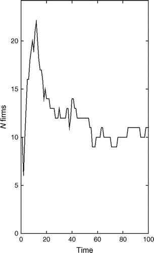
Before considering the aggregate results, it is useful to examine a single history of our model to understand the sources of variation in firm size distributions. To facilitate comparison, the demand function and the cost distribution is defined exactly as in the baseline experiments explained later, with P0 = 1, Q1 = 250, and unit costs ci drawn from the general beta distribution (α = 5, β = 5) in the interval [0.2, 0.8]. Each period, a cohort of 10 latent entrants draws a value from the cost distribution. The cost value received by each potential entrant determines whether that entrant has realized a cost value that allows it to be viable in the current market setting. In addition, as outlined earlier, the incumbent firms face the possibility of exit if their cost value is no longer viable. Incumbent firms that remain in the market calculate their target Cournot quantity level and adjust to that level from their current production as a function of the adjustment parameter δ. Figure 1 provides a history in the case of no noise, while Figure 2 provides a history where σ > 0 (σ = 0.01). Note that the introduction of “noise,” i.e. random shocks to firms’ cost value, does not exert a qualitative effect on these patterns. Both curves depicting industry evolution, as characterized by the number of firms at each point in time, provide the standard pattern of increasing aggregate quantity with the pattern of the number of firms over time consistent with an industry shakeout (Gort and Klepper 1982, Klepper and Graddy 1990).
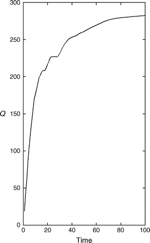
Notes. Rate of scale-adjustment, δ = 0.10. Firm-specific random shocks, σ = 0.
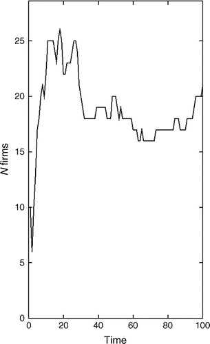
Notes. Rate of scale-adjustment, δ = 0.10. Firm-specific random shocks, σ = 0.
Notes. Rate of scale-adjustment, δ = 0.10. Firm-specific random shocks, σ = 0.
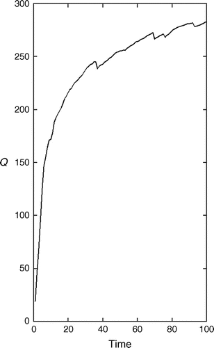
Notes. Rate of scale-adjustment, δ = 0.10. Firm-specific random shocks, σ = 0.01.
Notes. Rate of scale-adjustment, δ = 0.10. Firm-specific random shocks, σ = 0.01.
Notes. Rate of scale-adjustment, δ = 0.10. Firm-specific random shocks, σ = 0.01.
In the following, we present results from a systematic examination of our model. The results reported here are based on averages of 1,000 such histories with each ‘history’ spanning 1,000 discrete time steps. We use a baseline setting of an exponential demand curve with parameters, P0 = 1 and Q1 = 250, and set the default size of the cohort of potential entrants to NC = 10. Thus, each period, a cohort of NC firms considers entering the industry. Each member of this cohort is randomly assigned a unit cost value ci drawn from the general beta distribution (α = 5, β = 5) in the interval [0.2, 0.8]. A firm enters the industry if its cost value is less than the current market price of a unit of output. Thus, while the cohort size of potential entrants is held fixed over time, the number of actual entrants varies a great deal, with the typical pattern being that the set of entrants is equal or nearly equal to the number of potential entrants early on and declining over time. Each run of the model produces a particular history of an industry. The rate of scale adjustment δ is a critical parameter as it determines the extent to which firms adjust output in a systematic way. As δ approaches 1, the firms’ adjustment of output becomes instantaneous. We examine values of δ = {0.005, 0.01, 0.05, 0.10, 0.50, 1.00} and a range of σ values considering σ = {0, 0.001, 0.010, 0.025}. In addition, beyond these reported results, we have engaged in a large number of experiments with additional values of NC, Q1, as well as shape parameters and range of the underlying cost distribution. The results presented here are qualitatively robust to changes within a very broad range of these parameters.
Tables 1 and 2 provide a sense of the industry dynamics over a broad range of parameter values. The subset of parameter values that “dock” well with observed patterns (Gort and Klepper 1982, Dunne et al. 1988) correspond to settings with moderate to low rates of adjustment of firm capacity to its target value. In particular, Dunne et al. (1988, p. 503), report the entry and exit rates in the four-digit U.S. manufacturing industries over the period 1963–1982 (see the data in their Table 2). They find that the average entry rate over the entire period was 49.0%, or 38.6% if the smallest firms were deleted (firms that jointly produce 1% of the industry’s output). The corresponding exit rates were 46.4% (all firms) and 35.2% (small firms deleted). These numbers translate to average yearly entry and exit rates of 9.81% and 9.29%, respectively, including all firms, and 7.72% and 7.04% if small firms are deleted. Newer data, drawing from the Canadian economy, are consistent with these numbers as well. In particular, during the period of 2000–2008, the average yearly entry and exit rates in the Canadian economy were 10.8% and 9.0%, respectively (Ciobanu and Wang 2012). This link between the rate of capacity adjustment to industry dynamics points to an important, but arguably somewhat neglected factor in understanding industry dynamics (Knudsen et al. 2014).
|

Table 1: Industry Dynamics
| No. of firms | |||||||
|---|---|---|---|---|---|---|---|
| Delta | Sigma | t = 5 | t = 10 | t = 100 | t = 1,000 | Max. | Shakeout |
| 0.005 | 0.000 | 16.6 | 26.5 | 56.4 | 31.1 | 67.5 | 36.3 |
| 0.001 | 16.7 | 26.5 | 56.9 | 31.2 | 67.9 | 36.7 | |
| 0.010 | 16.6 | 26.3 | 56.1 | 28.2 | 66.1 | 37.8 | |
| 0.025 | 16.5 | 25.4 | 51.9 | 25.0 | 61.2 | 36.2 | |
| 0.01 | 0.000 | 16.7 | 26.5 | 39.8 | 29.0 | 57.7 | 28.7 |
| 0.001 | 16.5 | 26.4 | 39.9 | 29.0 | 57.7 | 28.7 | |
| 0.010 | 16.6 | 26.3 | 39.1 | 24.9 | 55.3 | 30.5 | |
| 0.025 | 16.3 | 25.4 | 35.0 | 21.1 | 51.1 | 30.0 | |
| 0.05 | 0.000 | 16.7 | 26.0 | 20.1 | 27.1 | 38.8 | 11.8 |
| 0.001 | 16.6 | 25.7 | 20.1 | 24.9 | 38.0 | 13.1 | |
| 0.010 | 16.5 | 25.6 | 18.8 | 12.2 | 31.9 | 19.7 | |
| 0.025 | 16.3 | 24.9 | 16.5 | 8.6 | 31.5 | 23.0 | |
| 0.10 | 0.000 | 16.5 | 21.8 | 18.7 | 27.1 | 32.6 | 5.5 |
| 0.001 | 16.5 | 21.9 | 18.8 | 26.8 | 33.0 | 6.1 | |
| 0.010 | 16.3 | 21.6 | 16.0 | 10.8 | 25.5 | 14.7 | |
| 0.025 | 16.3 | 21.1 | 12.7 | 7.2 | 25.0 | 17.8 | |
| 0.50 | 0.000 | 10.9 | 11.5 | 17.3 | 26.7 | 30.6 | 3.9 |
| 0.001 | 10.9 | 11.3 | 17.7 | 26.7 | 30.9 | 4.2 | |
| 0.010 | 10.8 | 11.0 | 11.0 | 9.7 | 17.1 | 7.4 | |
| 0.025 | 10.6 | 9.7 | 7.1 | 5.8 | 14.8 | 8.9 | |
| 1.00 | 0.000 | 8.4 | 10.3 | 17.4 | 26.8 | 30.5 | 3.7 |
| 0.001 | 8.6 | 10.4 | 17.5 | 26.6 | 30.4 | 3.9 | |
| 0.010 | 8.1 | 9.1 | 10.0 | 9.3 | 15.3 | 6.0 | |
| 0.025 | 7.6 | 7.5 | 6.0 | 5.3 | 12.3 | 7.0 | |
|
Table 2: Entry and Exit Over the Industry Lifecycle
| Delta | Sigma | Entry rates (%) | Exit rates (%) | Entry-Exit (%) | |||
|---|---|---|---|---|---|---|---|
| Phase | Phase | Phase | |||||
| 1 | 3 | 1 | 3 | 1 | 3 | ||
| 0.005 | 0.000 | 6.27 | 0.12 | 2.60 | 0.10 | 3.67 | 0.02 |
| 0.001 | 6.17 | 0.12 | 2.53 | 0.11 | 3.63 | 0.01 | |
| 0.010 | 6.35 | 0.13 | 2.63 | 0.14 | 3.71 | −0.01 | |
| 0.025 | 6.62 | 0.17 | 2.94 | 0.20 | 3.68 | −0.03 | |
| 0.01 | 0.000 | 9.06 | 0.14 | 3.73 | 0.12 | 5.33 | 0.02 |
| 0.001 | 9.08 | 0.14 | 3.72 | 0.12 | 5.36 | 0.02 | |
| 0.010 | 9.22 | 0.17 | 3.77 | 0.17 | 5.44 | 0.00 | |
| 0.025 | 9.66 | 0.23 | 4.23 | 0.26 | 5.43 | −0.03 | |
| 0.05 | 0.000 | 11.73 | 0.20 | 4.81 | 0.19 | 6.92 | 0.01 |
| 0.001 | 14.34 | 0.21 | 5.89 | 0.20 | 8.44 | 0.01 | |
| 0.010 | 19.35 | 0.38 | 8.03 | 0.43 | 11.32 | −0.06 | |
| 0.025 | 20.72 | 1.35 | 8.87 | 1.46 | 11.85 | −0.11 | |
| 0.10 | 0.000 | 2.97 | 0.13 | 1.55 | 0.15 | 1.42 | −0.02 |
| 0.001 | 3.85 | 0.15 | 1.88 | 0.17 | 1.98 | −0.01 | |
| 0.010 | 22.93 | 0.47 | 9.83 | 0.52 | 13.09 | −0.05 | |
| 0.025 | 26.69 | 1.84 | 11.56 | 2.05 | 15.13 | −0.20 | |
| 0.50 | 0.000 | 1.15 | 0.14 | 0.87 | 0.15 | 0.29 | −0.02 |
| 0.001 | 1.18 | 0.12 | 0.88 | 0.14 | 0.30 | −0.02 | |
| 0.010 | 15.88 | 0.60 | 9.78 | 0.66 | 6.10 | −0.06 | |
| 0.025 | 35.61 | 3.04 | 16.81 | 3.51 | 18.79 | −0.48 | |
| 1.00 | 0.000 | 1.19 | 0.17 | 0.90 | 0.18 | 0.29 | −0.01 |
| 0.001 | 1.19 | 0.16 | 0.90 | 0.18 | 0.29 | −0.01 | |
| 0.010 | 10.59 | 0.63 | 7.91 | 0.71 | 2.68 | −0.08 | |
| 0.025 | 78.88 | 3.93 | 6.62 | 4.69 | 72.26 | −0.76 | |
Given the range of values of the rate of adjustment (δ) and level of random shocks (σ) that correspond to the empirically observed broad patterns of industry entry and exit, the critical question becomes what these values imply for the growth dynamics, in particular the values of β and serial correlation that they imply. Before exploring this relationship, it is important to recognize that the model makes distinct predictions for these values at different epochs of the process of industry evolution. Per Gort and Klepper (1982) and Klepper and Graddy (1990), it is useful to demark industry dynamics by three epochs of pre-shake-out growth phase, the shakeout phase, and the post shake-out convergence to a steady state. The model suggests a systematic deviation from Gibrat’s law during growth and the shakeout phase of industry evolution. Early on in the industry history, firms grow in scale to realize the new market niche. During this period, we would expect, on average, to see a β value of greater than 1. Further, we would anticipate seeing positive levels of serial correlation as stronger firms that grew more in an earlier period continue to grow more. More broadly, it is in this early epoch that we would expect to see the empirically observable expression of firm heterogeneity as evolutionary theories would suggest (Nelson and Winter 1982, Klepper 1996). The implications for β values during the shakeout phase are ambiguous, as some firms began a secular decline that will ultimately lead to their exit, while a subset of firms will experience systematic growth as they fill the market space vacated by other firms. For the same reason, at the firm-level, we will see high levels of serial correlation during these first two epochs. In contrast, during the post shake-out convergence to a steady-state phase of maturity, we expect to see results that are consistent with Gibrat’s law.
Looking at Table 3, we see that in the phase of industry maturity, for the empirically relevant values of rate of adjustment (δ) and level of random shock (σ) (i.e., moderate rates of scale adjustment δ, and moderate to high rates of random shocks σ), that the value of β takes on the value of 1. Indeed, even in the absence of a firm-specific shock we see that β still takes on a value of 1. However, the pattern for the value of serial correlation is quite different. In the absence of a noise term, the value of serial correlation approaches 1; whereas, in the presence of a substantial noise term and a moderate to substantial rate of adjustment to the Cournot quantity value, the serial correlation approaches the empirically observed value of near zero.
|
Table 3: Serial Correlation and Slope of Growth Equation for Phase 1 (Growth Phase) and Phase 3 (Steady State) of Industry Lifecycle
| Delta | Sigma | Serial corr. | Beta value | ||
|---|---|---|---|---|---|
| Phase | Phase | ||||
| 1 | 3 | 1 | 3 | ||
| 0.005 | 0.000 | 0.76 | 0.99 | 1.02 | 1.00 |
| 0.001 | 0.74 | 0.89 | 1.02 | 1.00 | |
| 0.010 | 0.51 | 0.22 | 1.02 | 1.00 | |
| 0.025 | 0.23 | 0.07 | 1.01 | 1.00 | |
| 0.01 | 0.000 | 0.68 | 0.99 | 1.04 | 1.00 |
| 0.001 | 0.67 | 0.98 | 1.04 | 1.00 | |
| 0.010 | 0.47 | 0.18 | 1.04 | 1.00 | |
| 0.025 | 0.21 | 0.05 | 1.02 | 1.00 | |
| 0.05 | 0.000 | 0.67 | 0.98 | 1.09 | 1.01 |
| 0.001 | 0.53 | 0.42 | 1.10 | 1.00 | |
| 0.010 | 0.36 | 0.15 | 1.12 | 0.98 | |
| 0.025 | 0.15 | 0.12 | 1.07 | 0.97 | |
| 0.10 | 0.000 | 0.89 | 0.98 | 1.04 | 1.01 |
| 0.001 | 0.68 | 0.48 | 1.05 | 1.01 | |
| 0.010 | 0.27 | 0.07 | 1.16 | 0.98 | |
| 0.025 | 0.10 | 0.07 | 1.10 | 0.96 | |
| 0.50 | 0.000 | 0.91 | 0.97 | 1.03 | 1.01 |
| 0.001 | 0.15 | −0.05 | 1.03 | 1.00 | |
| 0.010 | 0.03 | −0.11 | 1.08 | 0.88 | |
| 0.025 | −0.01 | −0.10 | 1.00 | 0.81 | |
| 1.00 | 0.000 | 0.99 | 1.00 | 1.03 | 1.00 |
| 0.001 | 0.03 | 0.00 | 1.03 | 1.00 | |
| 0.010 | 0.01 | 0.00 | 0.73 | 0.52 | |
| 0.025 | 0.23 | 0.00 | 1.02 | 0.37 | |
Note. For each phase, averages were computed across all periods in that phase.
Consistent with our predictions, we see that in the early growth phase of the industry, β tends to take a value slightly above 1 while in the mature phase 3, for moderate values of δ, the value of β conforms well to the empirically predicted value of 1. Thus, we find that it is possible to reconcile the apparent contradictions posed by Geroski (2000). In the mature phase, when firms adjust their production scale, very small values of serial correlation are present when cost values are subject to even very small random perturbations. Furthermore, β, the parameter of the growth equation, takes on a value of 1 regardless of the rate of adjustment.
Although we were able to dock the synthetic data generated by the model to baseline regularities of entry and exit, what about the empirical linkages with this contrast of the fit of Gibrat’s law in relatively mature stages of an industry’s evolution and the lack of correspondence in early stages of industry evolution? Empirical analyses of industry evolution such as Klepper and Graddy (1990) generally either do not have measures of firm size or, as in the case of Agarwal et al. (2002), size is measured by plant capacity or other discrete categorical variables that do not readily link to a consideration of Gibrat’s law. However, the work of Dinlersoz and MacDonald (2009) does allow us to engage in a further docking and testing of the model’s empirical implications. Dinlersoz and MacDonald built a panel data set of 322 four-digit industries over a 35-year period. Critical for our purposes, they categorize these industries over time as corresponding to one of the three stages in the Gort-Klepper industry lifecycle: growth, shakeout, and steady-state. They examine how the skewness in firm size distributions changes in these different epochs and find that the size distribution is relatively skewed during the growth phase of the industry. In contrast, the skewness in the size distribution is more modest in the later industry maturity period. In contrast, they find that the standard deviation in size values increases in the phase of industry maturity. Table 4 examines these properties in the context of the synthetic data generated by our model. Indeed, these are the properties of the model results as well for moderate rates of scale adjustment (δ), and moderate to high levels of the shock term σ (σ values of 0.01 or 0.025). Thus, compared to the early epoch of an industry lifecycle, firm heterogeneity is increased, as measured by the standard deviation in size, while the skewness and kurtosis of the size-distribution is smaller in the mature stages of industry evolution. Furthermore, there is a reassuring consistency in that the parameter values (δ, σ) that dock with Dinlersoz and MacDonald’s (2009) observations on the standard deviation, skewness, and kurtosis of the firm-level size-distribution also fit the basic pattern of industry entry- and exit-rates as characterized by Dunne et al. (1988) and Ciobanu and Wang (2012).
|
Table 4: Four Moments of Size Distribution for Phase 1 (Growth Phase) and Phase 3 (Steady State) of Industry Lifecycle
| Delta | Sigma | Mean | Std. dev. | Skew | Kurtosis | ||||
|---|---|---|---|---|---|---|---|---|---|
| Phase | Phase | Phase | Phase | ||||||
| 1 | 3 | 1 | 3 | 1 | 3 | 1 | 3 | ||
| 0.005 | 0.000 | 1.00 | 3.08 | 0.94 | 2.79 | 1.85 | 1.18 | 7.58 | 4.00 |
| 0.001 | 1.00 | 3.08 | 0.94 | 2.79 | 1.87 | 1.18 | 7.67 | 4.01 | |
| 0.010 | 1.00 | 3.37 | 0.92 | 2.94 | 1.89 | 1.16 | 7.76 | 3.98 | |
| 0.025 | 1.04 | 3.82 | 0.93 | 2.96 | 1.70 | 0.99 | 6.66 | 3.60 | |
| 0.01 | 0.000 | 1.30 | 3.35 | 1.27 | 2.93 | 1.86 | 1.09 | 7.32 | 3.71 |
| 0.001 | 1.30 | 3.35 | 1.27 | 2.90 | 1.84 | 1.06 | 7.17 | 3.63 | |
| 0.010 | 1.29 | 3.87 | 1.23 | 3.04 | 1.87 | 1.02 | 7.40 | 3.62 | |
| 0.025 | 1.33 | 4.64 | 1.23 | 3.19 | 1.70 | 0.80 | 6.43 | 3.21 | |
| 0.05 | 0.000 | 3.02 | 3.66 | 2.78 | 3.03 | 1.40 | 0.98 | 4.90 | 3.43 |
| 0.001 | 2.90 | 3.92 | 2.72 | 3.05 | 1.46 | 0.96 | 5.13 | 3.41 | |
| 0.010 | 2.63 | 7.56 | 2.60 | 2.91 | 1.59 | 0.27 | 5.54 | 2.87 | |
| 0.025 | 2.64 | 11.45 | 2.54 | 5.20 | 1.49 | −0.30 | 5.17 | 2.30 | |
| 0.10 | 0.000 | 4.06 | 3.49 | 3.42 | 2.84 | 1.04 | 0.97 | 3.61 | 3.43 |
| 0.001 | 4.03 | 3.54 | 3.42 | 2.89 | 1.07 | 0.97 | 3.73 | 3.41 | |
| 0.010 | 3.80 | 8.51 | 3.68 | 2.98 | 1.39 | 0.24 | 4.64 | 2.74 | |
| 0.025 | 3.73 | 13.05 | 3.58 | 5.53 | 1.37 | −0.30 | 4.57 | 2.24 | |
| 0.50 | 0.000 | 4.49 | 3.49 | 3.63 | 2.83 | 0.93 | 0.95 | 3.33 | 3.38 |
| 0.001 | 4.47 | 3.49 | 3.57 | 2.81 | 0.91 | 0.95 | 3.30 | 3.39 | |
| 0.010 | 8.06 | 9.34 | 5.70 | 3.15 | 0.73 | 0.25 | 2.92 | 2.56 | |
| 0.025 | 8.85 | 16.10 | 7.16 | 6.16 | 0.80 | −0.12 | 2.89 | 2.07 | |
| 1.00 | 0.000 | 4.53 | 3.47 | 3.61 | 2.82 | 0.92 | 0.95 | 3.30 | 3.36 |
| 0.001 | 4.55 | 3.50 | 3.61 | 2.81 | 0.92 | 0.94 | 3.33 | 3.35 | |
| 0.010 | 9.64 | 9.87 | 5.60 | 3.65 | 0.43 | 0.15 | 2.54 | 2.43 | |
| 0.025 | 13.73 | 17.83 | 10.98 | 7.60 | 0.55 | 0.01 | 2.28 | 1.98 | |
Note. For each phase, averages were computed across all periods in that phase.
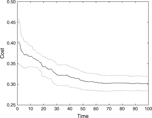
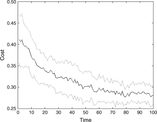
The motivating question for this exercise is whether firm-level heterogeneity is compatible with the growth dynamic regularities of near zero-correlation in growth rates and a growth parameter of 1. We have clearly addressed these latter two properties. Let us now directly consider the property of firm-level heterogeneity. Figures 1(c) and 2(c) do so, providing the distribution of cost values, plus and minus standard deviation from the mean, across time. We see a substantial level of persistent heterogeneity. Further, this heterogeneity is not simply a byproduct of firm-specific shocks. While firm-specific shocks to cost values do, to some degree, increase the level of variation in cost values, the basic heterogeneity is due to the fundamental process of the entry process and Cournot competition (cf., Lippman and Rumelt 1982, Klepper 1996, Knudsen et al. 2014).
Discussion
The analysis has examined some of the most basic and pervasive regularities about industry dynamics. The fact that firms have persistent differences (Syverson 2011) has, on its surface, appeared to be at odds with the regularities we observe regarding the growth dynamics of industry populations. Our modeling effort, however, reveals that these properties are in fact not inconsistent. We have used a stylized model of industry evolution to generate data on which we have applied the standard empirical analysis of firm growth rates. The model generates synthetic data that, when estimated using the standard methods in this domain, yield estimated results consistent with baseline regularities of industry and growth.
Firm differences play themselves out in the battle for market share—a battle that is attenuated by the Cournot recognition of relative market power. As the industry approaches steady-state equilibrium, heterogeneity is expressed in divergent cost values and market share. Growth rates, however, reflect off-equilibrium disturbances. In contrast, in the early stages of an industry’s evolution, firm-level heterogeneity is expressed in growth rates as well. Superior firms grow at a faster rate as they fill out the market niche. More generally, dynamic manifestations of heterogeneity are revealed when the industry is far from equilibrium. As the industry approaches equilibrium, heterogeneity is only revealed in the cross section (cost, market share, etc.) and not in the dynamics.
Further, the model helps to illuminate the empirical deviations that have been identified from Gibrat’s law (Evans 1987, Hall 1987, Bottazzi and Secchi 2006). The deviations from a process of random proportionate growth stem from the relatively rapid rates of growth of young and small firms. However, our work suggests that these anomalies may largely stem from the relationship between growth rates and the dynamics of industry evolution. The demography of an industry population is disproportionately composed of young, small firms at the outset of an industry’s development. Certainly, while there may be inter alia industry entrants (Klepper and Simons 2000, Helfat and Lieberman 2002), that at the level of overall firm size are of substantial scale, de novo entrants are both “young” and “small.” Thus, the industry population is heavily weighted with young and small firms at a point in the industry dynamics where our analysis indicates that the growth rate parameter takes on values in excess of 1.
More generally, the empirical analysis of firm growth, from the early work of Ijiri and Simon (1964 and 1967) onward, has been largely decontextualized from historical time and place. By that, we mean studies generally consist of panel data sets and while industry controls may be applied, where “industry” is identified by a SIC classification (typically at the four-digit level), these classifications are very poor proxies for industry membership where industry is conceived as a set of products and services with high rates of substitutability. A further characteristic of such panel data sets is that their beginning and end points tend to be rather arbitrary time markers. Thus, even if the SIC classification was a fairly good match of an underlying industry, the sample is, in most instances, likely to censor the early stage of the industry’s development where their evolutionary dynamics are most pronounced and the manifestation of firm heterogeneity in growth rates most visible.
The aggregate behavior of an industry population is not merely the sum of independent firm characteristics, as most treatments of Gibrat’s law have implicitly assumed. The structure of competition impacts the observed firm-level dynamics. When competitive forces are relatively weak in the early stages of an industry’s evolutionary dynamic, we see strong empirical manifestations of firm-level heterogeneity in the form of differential growth rates. It is when competitive dynamics are more binding at more mature stages of the industry, that firm-level heterogeneity is suppressed with respect to growth rates. However, even then, the observation of homogeneous and proportionate growth rates need not be at odds with firms being quite heterogeneous, having diverse cost values and associated market share. Firm heterogeneity and Gibrat’s law are not incompatible truths, but rather basic elements of a more unified understanding of firm and industry dynamics.
The authors appreciate the thoughtful and constructive feedback of the reviewers and senior editor.
Appendix. Outline of a Formal Explanation
Here we sketch a proof that can explain why even small random shocks caused by sequential adjustment or perturbations of cost values may cause zero serial correlation. Suppose firms are subject to random shocks in cost values so they adjust desired output upward or downward with equal probability. For simplicity, further assume that all adjustments are of unit size, so that differences in scale between two points in time are randomly distributed numbers drawn from the set {−1, 0, +1}. We wish to extract the covariance between the vectors Δ1 and Δ2, each containing differences in scale between two points in time:
This argument is readily extended to the case where random shocks to cost values are symmetrically distributed around a mean of zero. In that case, two equal sized adjustments of opposite signs occur with equal probability. Thus, we see that the condition necessary to produce unsystematic variation in firm size distributions, as measured by serial correlation, is that firms are subject to random shocks that make them scale up or down with equal probability. As we have shown, the source of such shocks can either be random firm-specific shocks in cost values, or a serial process of scale adjustment that involves ongoing mutual adjustments. Even though these shocks occur at random, it is easy to reconcile with a process where each firm systematically adjusts its scale according to its circumstance. That is, external shocks in a sense mask the underlying systematic nature of the adjustment process. Thus, we argue that the size of a firm at any time is more than just the sum of the whole history of shocks, which it has received since it was founded (Geroski 2000). Rather, the size of the firm is joint effect of sum of the history of the shocks the firm has received and the way it has reacted to those shocks.
1 Indeed, in our collaboration on this project we came to refer to these seemingly inconsistent properties as “Geroski’s paradox.”
2 We forego development of the elementary details, since they are well established in the literature (c.f., Sutton 1997).
3 This structure poses the potential for cost to fall below the value of zero. If a sequence of random draws were to result in a realized cost value that violates the bound of zero cost, then a new draw of the random noise term is carried out. In our computations, however, the probability that this occurs is small since σ2 ≥ 0.025. In the runs that underlie the subsequent analysis, this condition was never realized.
4 A more behaviorally plausible alternative would be for firms to form their Cournot conjectures regarding market price based on the prior period quantity choices by competitors. A Cournot model based on prior period output generates model results that are essentially the same as those provided here. A model that postulated conjectures as being some mixture of prior and current period product, a behavioral adjustment model, generates somewhat distinct behavior as the behavioral adjustment process is itself a source of “noise” in the process of industry dynamics. However, even in this case the qualitative properties characterized here continue to hold.
5 The serial correlation is defined when at least one firm changes output between consecutive time steps (1,2) and (3,4). Because of ongoing adjustment to entry and exit, this condition is almost always fulfilled in our model.
References
- (2002) The conditioning effect of time on firm survival: An industry life cycle approach. Acad. Management J. 45(4):971–994.Crossref, Google Scholar
- (2001) Zipf distribution of U.S. firm sizes. Science 293:1818–1829.Crossref, Google Scholar
- (2006) Explaining the distribution of firm growth rates. The RAND J. Econom. 37(2):235–256.Crossref, Google Scholar
- (2012) Firm Dynamics: Firm Entry and Exit in Canada, 2000 to 2008. Statistics Canada Catalogue no. 11-622-M. Ottawa, Ontario. The Canadian Economy in Transition. No. 22.Google Scholar
- (2009) The Growth of Firms: A Survey of Theories and Empirical Evidence (Edward Elgar, Cheltenham, UK).Crossref, Google Scholar
- (2009) The industry life-cycle of the size distribution of firms. Rev. Econom. Dynam. 12:648–667.Crossref, Google Scholar
- (1988) Pattern of firm entry and exit in U.S. manufacturing. Rand J. Econom. 19(4):495–515.Crossref, Google Scholar
- (1987) The relationship between firm growth, size, and age: Estimates for 100 manufacturing industries. J. Indust. Econom. 35(4):567–581.Crossref, Google Scholar
- (2000) The growth of firms in theory and practice. Foss N, Mahnke V, eds. Competence, Governance and Entrepreneurship (Oxford University Press, Oxford, UK), 168–186.Crossref, Google Scholar
- (1931) Les Inégalités Économiques (Librairie du Recueil Sirey, Paris).Google Scholar
- (1982) Time paths in the diffusion of product innovations. Econom. J. 92(367):630–653.Google Scholar
- (1987) The relationship between firm size and firm growth in the US manufacturing sector. J. Indust. Econom. 35(4):583–606.Crossref, Google Scholar
- (2002) The birth of capabilities: Market entry and the importance of pre-history. Indust. Corporate Change 11(4):725–760.Crossref, Google Scholar
- (1992) Entry, exit, and firm dynamics in long run equilibrium. Econometrica 60(5):1127–1150.Crossref, Google Scholar
- (1964) Business firm growth and size. Amer. Econom. Rev. 54(2):77–89.Google Scholar
- (1967) A model of business firm growth. Econometrica 35(2):348–355.Crossref, Google Scholar
- (1982) Selection and the evolution of industry. Econometrica 50(3):649–670.Crossref, Google Scholar
- (1996) Entry, exit, growth, and innovation over the product life cycle. Amer. Econom. Rev. 86(3):562–583.Google Scholar
- (1990) The evolution of new industries and the determinants of market structure. The RAND J. Econom. 21(1):27–44.Crossref, Google Scholar
- (2000) Dominance by birthright: Entry of prior radio producers and competitive ramifications in the U.S. television receiver industry. Strategic Management J. 21(10–11):997–1016.Crossref, Google Scholar
- (2006) Submarkets and the evolution of market structure. Rand J. Econom. 37(4):861–886.Crossref, Google Scholar
- (2014) Hidden but in plain sight: The role of scale adjustment in industry dynamics. Strategic Management J. 35(11):1569–1584.Crossref, Google Scholar
- (1982) Uncertain imitability: An analysis of interfirm differences in efficiency under competition. Bell J. Econom. 13(2):418–438.Crossref, Google Scholar
- (1997) How much does industry matter, really? Strategic Management J. 18:15–30.Crossref, Google Scholar
- (1982) An Evolutionary Theory of Economic Change (Belknap Press, Cambridge, MA).Google Scholar
- (1991) How much does industry matter? Strategic Management J. 12(3):167–185.Crossref, Google Scholar
- (1985) Do markets differ much? Amer. Econom. Rev. 75(3):341–351.Google Scholar
- (1997) Gibrat’s legacy. J. Econom. Lit. 35(1):40–59.Google Scholar
- (2011) What determines productivity? J. Econom. Lit. 49(2):326–365.Crossref, Google Scholar
Thorbjørn Knudsen is a professor of organization design at the University of Southern Denmark (SDU) where he heads the Strategic Organization Design Unit and is co-director of the Danish Institute for Advanced Study (DIAS). His research interests center around evolutionary and adaptive processes in organizations and the way organization design can shape these processes.
Daniel A. Levinthal is the Reginald H. Jones Professor of Corporate Strategy at the Wharton School, University of Pennsylvania. His research focuses on questions of organizational adaptation and industry evolution, particularly in the context of technological change.
Sidney G. Winter is the Deloitte & Touche Professor of Management, Emeritus, at The Wharton School, University of Pennsylvania. His research focus has been on the study of management problems from the viewpoint of evolutionary economics.

