Asymptotic Optimality of Switched Control Policies in a Simple Parallel Server System Under an Extended Heavy Traffic Condition
Abstract
This paper studies a two-class, two-server parallel server system under the recently introduced extended heavy traffic condition, which states that the underlying “static allocation” linear program (LP) is critical, but does not require that it has a unique solution. The main result is the construction of policies that asymptotically achieve previously proved a lower bound, on an expected discounted linear combination of diffusion-scaled queue lengths and are therefore asymptotically optimal (AO). Each extreme point solution to the LP determines a control mode—that is, a set of activities (class-server pairs) that are operational. When there are multiple solutions, these modes can be selected dynamically. It is shown that the number of modes required for AO is either one or two. In the latter case, there is a switching point in the (normalized) workload domain, characterized in terms of a free boundary problem. Our policies are defined by identifying pairs of elementary policies and switching between them at this switching point. They provide the first example in the heavy traffic literature where weak limits under an AO policy are given by a diffusion process where both the drift and diffusion coefficients are discontinuous.
Funding: R. Atar is supported by the Israel Science Foundation [Grant 1035/20].
1. Introduction
1.1. Background
Parallel server systems (PSSs) are queueing control problems in which a number of servers offer service to customers of different classes, and choices as to which customer class each server is dedicated to are made dynamically. Since its introduction in Harrison and López (1999), its study in heavy traffic has attracted much attention, due to its simple structure, its practical significance, and the theoretical challenges it poses. The problem formulation in Harrison and López (1999) includes a key assumption, referred to as the heavy traffic condition (HTC), which states that an underlying “static allocation” linear program (LP) satisfies a critical load condition and that it has a unique solution. Whereas critical load is universally considered a defining condition of any notion of heavy traffic, uniqueness of solutions has been assumed mainly because it simplifies the mathematical treatment. The extended HTC (EHTC), which merely states that the LP is at criticality, but does not require uniqueness, has recently been introduced in Atar et al. (2024) in order to address a considerably broader notion of heavy traffic. The main result of Atar et al. (2024) is a lower bound on the asymptotically achievable cost in a general PSS under the EHTC. This paper focuses on the two-class, two-server PSS referred to in this introduction as the 2 × 2 PSS, which is the simplest case in which the EHTC is strictly broader than the HTC. The goal is to complement the results of Atar et al. (2024), in this case by constructing policies that asymptotically achieve the lower bound, which, hence, are asymptotically optimal (AO) in heavy traffic.
The structure of the 2 × 2 PSS is as follows. Each of the two servers is capable of serving each of the two classes. The classes (respectively, servers) are usually indexed using the symbol i (respectively, k) and activities, namely, class-server pairs, by . Arriving customers await service in class-based queues and, upon receiving a single service, leave the system. The control decisions consist of routing (determining which server serves each customer) and sequencing (determining the order in which they are served). The rates of arrivals of customers of the two classes are denoted by , i = 1, 2, and the rates of service at each of the four activities are denoted by , where n denotes the usual heavy traffic parameter. These rates are assumed to be asymptotic to and , for some given λi, , μik, . The cost consists of an expected infinite horizon discounted linear combination of the two queue lengths and is rescaled at the diffusion scale.
Whereas the cost and, consequently, the notion of AO are set up at the diffusion scale, the underlying LP alluded to above addresses the behavior of the PSS at the fluid, or law-of-large-numbers (LLN), scale. Posed in terms of the first-order parameters, λi, μik, it is concerned with the mean fraction of time devoted by each server to each class. When the LP has a unique solution, at least one activity is nonbasic, in the sense that the fraction allocated to it is zero. The so-called graph of basic activities (GBA), formed by the activities with positive allocation fraction, is static. In this case, the critical load condition dictates that any policy not adhering to this solution, in the sense of effort allocation, causes the total queue length to blow up and, in particular, cannot be AO. Under policies that adhere to this solution, the LLN assures that the aforementioned fractions of effort converge to those given by the LP solution (a necessary, but certainly not sufficient, condition for AO). When there are multiple LP solutions, a result from Atar et al. (2024) states that for the 2 × 2 PSS, the space of solutions, denoted by , forms a line segment in the space of 2 × 2 matrices (where “ch” denotes the convex hull). In each of the two extremal solutions, there is again at least one nonbasic activity. We refer to these two extreme points as control modes, or simply modes. For similar reasons, any policy that does not lead to an unbounded cost should keep the system critically loaded at all times, and, thus, asymptotically, the fractions of effort will vary dynamically within . In the control literature, a control process that takes values only at the vertices of the action space is called a bang-bang control. The analogue of this notion in our setting is a policy for which the limiting fractions of effort take values only in , switching between the two extremal solutions. Some of the policies introduced in this paper are designed to act that way.
Contrary to the setting where the HTC holds, it is impossible to construct an AO policy based only on the first-order data under the EHTC. A second-order approximation of the PSS, which is often referred to as a Brownian control problem (BCP), is required. The BCP represents a diffusion limit of the PSS, in which Brownian motion (BM) replaces stochastic fluctuations associated with cumulative arrival and service processes. Closely related to the BCP is another diffusion control problem, called a workload control problem (WCP). Obtained by a certain projection of the BCP, it is a control problem in which the process is one-dimensional, representing the total workload asymptotics. The structure of the WCP obtained is quite simple to describe. The state process is a reflected diffusion on , with controlled drift and diffusion coefficients, , where the control process, , takes values in , and is an affine map. The cost is given as an expected discounted version of the state process itself. By a standard argument based on the Hamilton-Jacobi-Bellman (HJB) equation, there exists an optimal bang-bang control for the WCP. There can therefore be two possibilities for the WCP solution: the single-mode case, where one of the modes is always used, and the dual-mode case, where both modes are used by the optimal control in different parts of the state space. Note that in this case, the GBA can be changed dynamically. The HJB equation also reveals the structure of the feedback function from state to control. This particular HJB equation was solved in Sheng (1978). It was shown that in the dual-mode case, there is a switching point , such that one of the modes is used when the state is below and the other otherwise. The HJB equation can be viewed, in this case, as an equation involving a free boundary, in which the solution is a pair, where one component is the value function and the other is . The results of Sheng (1978) also characterize as the unique solution to an explicit equation, as well as a solution to the HJB equation.
Our policies are obtained by “translating” the WCP solution. In the case of a single mode, the prescribed policy corresponds either to a threshold policy of the form that first appeared in Bell and Williams (2001) (see below) or a simple priority policy, depending on the mode used and the cost. In the dual-mode case, pairs of elementary policies are identified, which are combined together to form switched control policies, so that one is active when the normalized workload process is below the switching point and the other above it. In each case, the policy is designed to meet the target allocation efforts determined by the corresponding mode, and the set of operational activities is restricted by the corresponding GBA.
The paper closest to ours is the aforementioned Bell and Williams (2001), which studies a two-server, two-class PSS with three activities. This PSS is known as an “N” network because upon relabeling, the activities are given by (1, 1), (1, 2), and (2, 2), forming the symbol N. (See Figure 1(a).) In this network, the number of solutions to the LP cannot exceed one, and, thus, the requirement of a unique solution does not pose a restriction. In an earlier work, Harrison (1998), it had been observed that when the larger “” value is in class 1, the BCP solution suggests that the queue length of class 1 customers and the idleness process at server 1 should both converge to zero at the diffusion scale and that a simple priority policy does not achieve this. In Bell and Williams (2001), this was addressed by putting a threshold on class 1 queue length that, when exceeded, server 2 prioritizes class 1, and otherwise it prioritizes class 2. The size of the threshold must converge to zero at the diffusion scale so as to achieve the first goal. To achieve AO of a threshold policy with logarithmic (in n) size threshold, as used in Bell and Williams (2001), the interarrival and service times are assumed there to possess exponential moments. (More on the history of the problem and the works that contributed to its development can be read in Atar et al. 2024.)
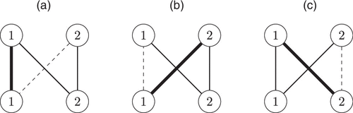
Notes. Graph (a) corresponds to a mode in canonical form. Graphs (a) and (b) correspond to a pair of modes where the nonbasic activity switches a class, whereas in graphs (a) and (c), it switches a server. The pair (b) and (c), in which the nonbasic activity switches both a class and a server, is neither class- nor server-switched.
As already mentioned, one of the policies we implement is a threshold policy similar to the one used by Bell and Williams (2001). However, our assumptions are positioned differently with respect to the threshold-moment tradeoff, assuming a larger (still ), polynomial size threshold, but requiring only a polynomial moment assumption. We assume moment assumptions for all of our policies except the single-mode threshold policy and the dual-mode policies that employ the threshold policy when the workload is above . For these, a finite -th moment is assumed, where the number is indicated explicitly. Another difference between our results and those of Bell and Williams (2001) is that our policies do not use preemption. Although the policy introduced in Bell and Williams (2001) uses preemption, it is plausible that an analogous nonpreemptive policy is also AO under similar conditions; see Corollary 2.15 and Remark 2.16. In this paper, our choice not to use preemption leads to nontrivial issues in the dual-mode case. Instead of a simple switching between elementary policies when the workload crosses , it is sometimes the case that one must wait for a particular server to become available before switching. This is described in Section 5.1.3.
It is also worth mentioning that we have argued in Atar et al. (2024) that the AO of the threshold policy from Bell and Williams (2001) extends beyond the HTC to the case of multiple solutions and a single mode (under some assumptions, which include the existence of exponential moments).
Besides the objective to break the uniqueness barrier, an additional source of motivation for this work stems from the relation between nonuniqueness and service rate decomposability. As stated in Lemma 2.1, for the 2 × 2 PSS, the LP exhibits multiple solutions if and only if the service rates decompose as . Service rates decompose this way when the mean size of a job is characteristic to the class (and then αi is the reciprocal mean) and each server has its own processing speed (here given by βk). As the HTC does not hold under decomposability, this important class of service rates has been left out by earlier work.
1.2. Results
The description of the policies given above is only a sketch. There are nontrivial issues that arise regarding the need to “patch” two policy types, requiring us to slightly modify the policies, where the details differ from one pairing to another.
The main result states that, under the prescribed policies, the rescaled workload process converges in law to the diffusion process that solves the WCP, and these policies are AO. As far as convergence is concerned, in addition to the “standard” issues involved in proving state-space collapse, we need to deal with issues related to switching control modes at . Moreover, to obtain AO from weak convergence, uniform integrability needs to be established, and it is here where the and moment assumptions are used.
An approach to proving convergence to a diffusion with discontinuous coefficients, addressing especially the technicalities involved with the discontinuity of the diffusion coefficient, was developed in Krylov and Liptser (2002), going beyond the general framework for convergence of semimartingales, such as that from Liptser and Shiriaev (1977). Whereas the tools from Krylov and Liptser (2002) are not directly applicable in our setting, an argument that, as in Krylov and Liptser (2002), shows that the time spent near the discontinuity set is negligible is also at the basis of our proof. The paper Krylov and Liptser (2002) also gives an example of a queueing model whose scaling limit yields a diffusion process with discontinuities in both drift and diffusion coefficients. Our dual-mode case provides what seems to be the first example where this occurs under an AO policy of a queueing control problem (for AO in heavy traffic leading to discontinuity in the drift only, see Atar and Lev-Ari 2018).
1.3. Organization of the Paper
In Section 2.1, we describe our model and the control problem associated with it in more detail. The LP and the extended heavy traffic condition are introduced in Section 2.2, and preliminary results about the LP from Atar et al. (2024) are stated. In Section 2.3, the WCP and the associated HJB equation are introduced, and in Proposition 2.6, it is stated that there exists a unique classical solution to the HJB equation. This proposition also provides a condition that determines whether an optimal solution to the WCP must employ a single mode or two modes (not to be confused with the number of modes in the space of LP solutions, which is always two under multiplicity) and asserts that in the dual-mode case, there exists a single switching point in workload space. We also present in this section the lower bound from Atar et al. (2024) stated in Theorem 2.4. The main result is stated in Section 2.4. The definitions of the proposed policies appear first, and then, in Theorem 2.13, the weak convergence and AO results are stated. Numerical results are presented in Section 2.5.
In Section 3, we state and prove some results related to the static allocation LP, providing, in particular, explicit expressions for the extreme points of the set of optimal solutions. Development of the WCP is carried out in Section 4. Preliminary results proved in Atar et al. (2024) in a general case are included in this section. This section also contains proofs of results related to the HJB equation, some of which rely on Sheng (1978).
The proof of our main result, Theorem 2.13, is the subject of Section 5. In Section 5.1, we present the general scheme for proving Theorem 2.13; the weak convergence result is stated in Theorem 5.1. We then present four propositions that are used for the proof. Each proposition corresponds to a specific section and step of the proof. Proposition 5.3, in Section 5.2.2, proves uniform integrability; state space collapse is proved in Proposition 5.4 in Section 5.2.3; a key nonidling property is proved in Proposition 5.5 in Section 5.2.4; and a “fast switching” property, showing the aforementioned property that the process spends asymptotically negligible time near the discontinuity, is proved in Proposition 5.6 in Section 5.2.6. Appendix A contains proofs of several lemmas stated earlier. Appendix B presents expressions from Sheng (1981) for the solution to the HJB equation. Finally, Appendix C contains a result providing symmetry conditions under which a single mode control is optimal.
1.4. Notation
, and are the sets of natural, real, and, respectively, nonnegative real numbers. For and denote the maximum and minimum of a and b, respectively, and . For a set A, denotes its indicator function. For , and , and
For , the notation stands for . For real-valued functions and processes, the notation X(t) is used interchangeably with Xt. Given a Polish space E, and denote the spaces of E-valued, continuous and, respectively, càdlàg functions on , equipped with the topology of convergence uniformly on compacts and, respectively, the J1 topology. Denote by and the subset of and, respectively, , of nonnegative, nondecreasing functions and by the subset of of functions that are null at zero. Write for convergence in law. A sequence of processes with sample paths in is said to be C-tight if it is tight and the limit of every weakly convergent subsequence has sample paths in almost surely (a.s.). The letter c denotes a deterministic constant whose value may change from one appearance to another.
2. Model and Main Results
The setup and results presented in this section have quite a few ingredients, as already mentioned in the introduction: the LP and modes, the diffusion scaling, the WCP and HJB equation, the switching point , and threshold and switching policies. Before going into the details, we provide a roadmap. The two-class, two-server system, introduced in Section 2.1, is indexed by n and is observed at the diffusion scale. The assignment of jobs from the different classes to different servers is regarded as a control policy. A cost functional is considered, given by the expected discounted weighted sum of queue lengths, also rescaled at the diffusion scale; see Section 2.6. The weights of the queue lengths are given by a vector (h1, h2).
In order to formulate a policy-independent condition for heavy traffic, an LP (2.7) is introduced, involving first-order arrival and service rates, where the variable to be determined is a 2 × 2 allocation matrix describing the (first-order) fraction of effort each server dedicates to each class. It is assumed to be at criticality, in the sense that servers are fully occupied, but queue lengths stay balanced. In that regard, we adopt the heavy traffic notion of Harrison and López (1999) and many other papers that followed, with one important distinction: We do not assume that there is a unique allocation matrix that maintains criticality—that is, there may be multiple LP solutions. When there are multiple solutions, they are all given as convex combinations of two allocation matrices (Lemma 2.1), which we call modes. Because earlier work has addressed the unique solution case, we only treat the case of multiple solutions (Assumption 2.2). A result from Atar et al. (2024) states that under this assumption, the first-order rates μik are necessarily decomposable as . Each of the modes induces a so-called graph of basic activities, as in Figure 1. The parameters αi and the structure of the graphs influence the type of control policy to be proposed.
The WCP (2.16) and (2.17) is a control problem for a diffusion process in dimension 1, in which both the drift and the diffusion coefficient are controlled by a control process that takes values in the space of allocation matrices. The values of these coefficients, evaluated at the two modes, are denoted bm and, respectively, σm, m = 1, 2. The WCP formally describes the control problem associated with the PSS at the diffusion limit, and its control process represents the dynamic selection of the mode at which the PSS operates. The significance of the WCP has two aspects. First, as was shown in Atar et al. (2024), its solution gives a lower bound on the PSS cost asymptotics under any sequence of control policies (Theorem 2.4). Accordingly, any policy that achieves this bound is AO. Second, it suggests how AO policies should be structured. In particular: (a) State space collapse should hold, which, in our setting, involves two properties that should hold up to a level negligible at diffusion scale: (i) Both servers should be busy whenever there is any work in the system, and (ii) all queue length should be kept in the class i that minimizes . Roughly speaking, (ii) implies that the class that maximizes should be prioritized. This type of sequencing policy is known as a rule. (But, as shown by Harrison 1998 and Bell and Williams 2001, something more than a simple priority policy may be needed here in order to accomplish (i).) (b) When, for either or , one has and , only mode m should be used. Otherwise both modes should be used, by dynamically selecting them at different parts of the state space. The partition of the state space is defined via a switching point : When the diffusion-scaled workload is below , the mode m with should be used; otherwise, . Determining this switching point is done by solving an HJB equation, (2.18) and (2.19).
The construction of an AO policy must take into account several considerations: whether to operate in one or two modes and, in the latter case, their ordering in workload space; which class has high priority; and the structure of the graph of basic activities for each of the modes. Different types of policies apply in different cases (Definitions 2.9, 2.10, 2.11, and 2.12). The main result states that these policies are AO and that the normalized workload converges weakly to the diffusion process given by the WCP state process under an optimal control (Theorem 2.13).
2.1. Queueing Model, Scaling, and Queueing Control Problem
The model under consideration is as in Atar et al. (2024), specialized to the case of two job classes, two servers, and four activities. We will refer to it as the 2 × 2 PSS when there is need to distinguish it from the general PSS treated in Atar et al. (2024). The symbol is used as a generic index to a class and to a server. For a general PSS, an activity is a class-server pair (i, k), where server k is capable of serving class i. In this paper, it is assumed that each server is capable of serving each class; hence, there are four activities. They are labeled by (i, k) or sometimes by .
The model consists of a sequence of systems, indexed by , that are all defined on one probability space . For the nth system, one considers the following processes. The processes denoted and represent arrival and potential service counting processes. That is, is the number of arrivals of class i jobs until time t, i = 1, 2, and is the number of service completions of class i jobs by server k, by the time server k has devoted t units of time to class i, i = 1, 2, k = 1, 2. Next, , and denote queue length, cumulative idleness, departure, and cumulative busyness processes. In other words, is the number of class i customers in the system at time t, is the cumulative time server k has been idle by time t, is the number of class i departures from server k, and is the cumulative time devoted by server k to class i. The process takes the form , where is the fraction of effort devoted by server k to class-i jobs at t. In particular, for every k. Thus, is referred to as the allocation process.
The aforementioned arrival and potential service processes are constructed as follows. Arrival rates and service rates are given, satisfying, for some constants , ,
It is assumed, moreover, that the six processes are mutually independent and have strictly positive interarrival distributions and right-continuous sample paths. The independent and identically distributed interarrivals of and are denoted by and , respectively, and those of the accelerated processes and are given by
The system is assumed to start empty; that is, for all n. Simple relations between the processes are
The tuple is referred to as the stochastic primitives. In our formulation, we will consider Tn as the control process (equivalently, the allocation process may be regarded the control). In view of Equations (2.2), (2.3), and (2.4), given the stochastic primitives, the control uniquely determines the processes Dn, Xn, In. Let an additional process be defined on the probability space denoted by , taking values in a Polish space and assumed to be independent of the stochastic primitives, for each n (there is no need to let vary with n, as the primitives are all defined on the same probability space). It is included in the model in order to allow the construction of randomized controls; for more details about its potential use, see Atar et al. (2024, remark 2.1.ii).
The process Tn is said to be an admissible control for the queueing control problem (QCP) for the n-th system if for each (i, k), has sample paths in that are 1-Lipschitz, and the associated processes Dn, Xn, and In given by (2.2), (2.3), and (2.4) satisfy (2.5); furthermore, Tn is adapted to the filtration defined by . Denote by the collection of all admissible controls for the QCP for the n-th system. As argued in Atar et al. (2024, remark 2.1.i), this definition allows for the control to depend on the history of all processes involved in the model (in addition to the auxiliary randomness ).
The queue-length process normalized at the diffusion scale is defined by . The cost of interest for the n-th system is given by
This completes the description of the queueing models and QCP. The complete set of problem data consists of the stochastic primitives mentioned above and the collection of parameters
We sometimes refer to as the first-order data and to as the second-order data.
2.2. The Linear Program and Extended Heavy Traffic Condition
Given the first-order data , , consider the following linear program for the unknowns and .
Minimize ρ subject to
Denote the optimal objective value of (2.7) by .
The extended heavy traffic condition is broader than the heavy traffic condition that has been extensively used in the literature, which requires, in addition to , that there be a unique corresponding ξ.
Under the EHTC, any solution is of the form . Let denote the subset of , for which the set of all solutions is given by . We say that the EHTC with multiplicity (EHTCM) holds if the EHTC holds and the LP has multiple solutions (that is, there exist two distinct pairs and satisfying (2.7)). Following Atar et al. (2024), we say that the service rates μik are decomposable if for all i, k, for some constants αi and βk.
A matrix is called column-stochastic if for both k = 1, 2. A column-stochastic matrix is called a mode if (at least) one of its columns is either or . A mode is said to be degenerate if it has more than one zero entry; otherwise, it is said to be nondegenerate. A pair of nondegenerate modes is said to be a class-switched (server-switched) pair of modes if the zero entries in the two modes are in distinct rows but the same column (respectively, distinct columns but the same row). For example, the graphs in Figure 1, (a) and (b) correspond to a class-switched pair of modes, whereas those in Figure 1, (a) and (c) correspond to a server-switched pair.
The following condition will be referred to as the nondegeneracy condition, namely,
The following is proved in Section 3.
Let the EHTC hold.
For any solution , ξ is column-stochastic.
The LP (2.7) has multiple solutions if and only if are decomposable.
If the LP has multiple solutions, then there exists a pair of modes such that
(2.9)If the LP has multiple solutions and the nondegeneracy condition (2.8) holds, then both and of (2.9) are nondegenerate. Moreover, they form either a class-switched or a server-switched pair.
The main result will be proved under the following.
The EHTCM holds.
The nondegeneracy condition (2.8) holds.
Note that the case where the EHTC holds, but EHTCM does not hold, is already covered in the work Bell and Williams (2001), although, as mentioned in the introduction, under different assumptions on preemption and moment conditions. (See Corollary 2.15 and Remark 2.16 for implications of our results to the case where uniqueness holds and more on the relation to Bell and Williams 2001 in that case.)
In view of Lemma 2.1(2), under Assumption 2.2, the rates are decomposable. Thus, , and clearly, there is a degree of freedom in choosing and . In this paper, we will always assume that they are chosen so that , and it is easy to see that, given , this normalization uniquely determines these parameters.
It is also guaranteed by the lemma that, under Assumption 2.2, the extreme points of are two nondegenerate modes forming a class- or a server-switched pair. Once a labeling of these modes has been fixed, we will sometimes slightly abuse the terminology by referring to them as modes 1 and 2, rather than modes and .
In earlier work on PSS, under the assumption that the LP has a unique solution , activities are categorized as basic or nonbasic according to the positivity of the fraction allocated to them by ; that is, an activity (i, k) is basic if and nonbasic if . We extend this terminology to the case of multiple solutions as follows. For , an activity (i, k) is said to be basic in mode m if the allocation associated to it by this mode does not vanish, namely, . If (respectively, ) it is said to be nonbasic (respectively, full) in mode m.
Figure 1 demonstrates the second part of Lemma 2.1(4)—namely, that a pair of modes can be class-switched, as in Figure 1, (a) and (b), or server-switched, as in Figure 1, (a) and (c), but the LP does not give rise to a pair such as Figure 1, (b) and (c). The terms class-switched and server-switched will sometimes be abbreviated as “CS” and “SS.”
A mode is said to be in canonical form if its first column is . It is clear by the definition of a mode that it is always possible to relabel the classes and the servers so that a given mode is in canonical form and that if the mode is nondegenerate, there is only one such relabeling. The graph of a mode in canonical form is shown in Figure 1(a). Because of its resemblance to the symbol N, this form is sometimes called an N-system.
If the EHTCM holds, but (2.8) does not—that is, there exist i, k such that —the situation is different: at least one of the modes will be degenerate—that is, have two nonbasic activities (see Lemma 3.1). In the terminology of linear programming, this corresponds to a case where one of the basic solutions of the LP (2.7) is degenerate (cf. Goldfarb and Todd 1989, definition 3.1). The degenerate case is not covered in this paper. The key difficulty in the degenerate case is that, in at least one of the modes, the servers do not communicate in the graph of basic activities, so the pooling required to reach the cost lower bound is not possible. (See Atar et al. 2024, section 2.4 for a more detailed discussion of this issue.)
Under Assumption 2.2, both modes have a single nonbasic activity. Then, given a mode, the graph of basic activities has exactly three edges, and one can speak of the single-activity class (the one associated with only one nonbasic activity), the dual-activity class, and, similarly, the single- and dual-activity server. These terms allow us to refer to the roles of classes and servers in the graph without considering a particular labeling. It is also useful to accompany these terms with matching notation. For a mode ξ, let the single- (respectively, dual-) activity class be denoted by (respectively, ), and, similarly, let the single- (respectively, dual-) activity server be denoted by (respectively, ).
The following example, which corresponds to examples (A) and (B) in Atar et al. (2024), should help to make the above ideas more concrete.
Let be given by
Then, μik are decomposable as , where and . For , consider two cases—namely,
The linear program takes the form: Minimize ρ subject to
The solutions to the LP were calculated in Atar et al. (2024), and it was found that, in both cases, , and the two modes are given by
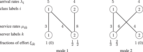
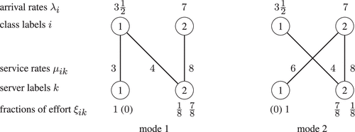
2.3. Workload Control Problem
The WCP was derived and studied in Atar et al. (2024) under the EHTC. We describe this problem in the special case needed here—namely, under the setting of a 2 × 2 PSS and assuming that the EHTCM holds. In particular, as mentioned above, the parameters are uniquely determined by the problem data. Define the workload process and its scaled version as
(It follows from Atar et al. 2024, lemma 2.4(2) that (2.11) agrees with the definition of Wn and given in Atar et al. 2024). Let the process that appears in the definition of the Cost (2.6) be denoted by
Throughout, denote by the two distinct indices for which
Let also
It was shown in Atar et al. (2024) that the asymptotics of the pair are governed by a state-control pair of processes , where Z is a one-dimensional controlled diffusion given by
is a control process, B is a standard BM (SBM), L is a reflection term at zero, and . A precise definition is as follows.
A tuple is said to be an admissible control system for the WCP with initial condition z if is a filtered probability space; B, , Z, and L are processes defined on it; B is a SBM and an -martingale; is -progressively measurable taking values in and satisfying ; Z is continuous nonnegative and -adapted; L has sample paths in and is -adapted; and Equation (2.16) and the identity are satisfied -a.s.
Denoting by the collection of all control systems for the WCP with initial condition z, the cost and value are defined as
The significance of the WCP lies in the fact that it provides a lower bound on the large n asymptotics of the n-th system value. More precisely, the main result of Atar et al. (2024), when specialized to the 2 × 2 PSS, states the following.
(
To prove this result, one only needs to verify that the assumptions from Atar et al. (2024) hold under Assumption 2.2. This is done in Section 3.
The general result from Atar et al. (2024) does not assume multiplicity and, moreover, uses different notation based on the formulation of a dual to the LP. In the 2 × 2 setting with multiplicity, the lower bound from Atar et al. (2024) reduces to the above expression given in terms of the parameters in place of the dual.
In view of Theorem 2.4, a sequence of admissible controls for the QCP, also referred to as a sequence of policies, is said to be asymptotically optimal if
2.3.1. A Heuristic Discussion of the WCP and Sheng’s Tortoise–Hare Problem.
The WCP is important not only because it provides a lower bound on performance, but also because one can learn from it how to construct a policy for the queueing model that performs near optimality. This problem has been solved completely. Before presenting its solution, we discuss its nature informally. Assume first that the pairs and are such that , while . Then, it is intuitively clear and can be shown by a simple coupling that is minimized by always using mode 1, because it has a smaller drift. Next, consider the case where b1 = b2, but . Mode 2 has greater variance, and, thus, one expects that the constraining mechanism, causing the diffusion to bounce back from the boundary, will be more active under mode 2 than under mode 1. Hence, again, using mode 1 at all times is optimal. More generally, mode 1 is optimal when and .
A more interesting case is when but , referred to in Sheng (1978) as the tortoise–hare problem. It seems reasonable to use the mode with smaller drift when the diffusion process is far from the origin and switch to the mode with smaller variance when it is close to the origin, where the aforementioned boundary effect is more prominent.
These heuristic arguments were validated rigorously in Sheng (1978). In particular, in the case , it was shown that there exists a point such that it is optimal to select mode 2 (resp., 1) when Zt is in (resp., ). The identification of and the proof of the result were based on an HJB equation. The precise details are as follows.
2.3.2. The HJB Equation.
The value function can be characterized in terms of an HJB equation (see Fleming and Soner 2006 for an introduction to the subject). To present this equation, for , let
Given a C2 function u, denote , m = 1, 2, and .
The following two conditions play an important role in what follows. They correspond to the two cases discussed above and will be referred to as the single-mode case and, respectively, the dual-mode case (not to be confused with uniqueness and multiplicity of the LP solution):
The C2 smoothness of the value function is tied to the question of existence of a classical solution to the HJB equation. Owing to the uniform ellipticity ( at both and ), one can show that a classical solution uniquely exists (Atar et al. 2024, proposition 2.5), a type of result that, in the general context of optimal switching of a diffusion process, has been called the principle of smooth fit. The results of Sheng (1978) alluded to above shed more light on the specific problem at hand, providing structural properties (parts 2 and 3 of the result below) that are harder to obtain via the general approach.
The proof of this result appears in Section 4. Some details on the construction from Sheng (1978) (as corrected in Sheng (1981), by which parts 2 and 3 above were proved, appear in Appendix B.
Further terminology is as follows. In the single-mode case, the mode for which m satisfies (2.20) will be referred to as the active mode and denoted ξA because the above result indicates that it is optimal to always select . In the dual-mode case, the modes and for which and m satisfy (2.21) will be referred to as ξL, the lower- and, respectively, ξH the higher-workload mode, and as the switching point. These terms refer to the fact that the result suggests that it is optimal to select (respectively, ) when (respectively, ).
We go back to Example 2.3, focusing on case (A), adding now information on the second-order data. Assume that the squared coefficients of variation and are all one except . Set both to zero. As for , consider two cases. In case (A1), all are set to zero. In case (A2), they are all zero except . For each of the modes, computing the drift and squared diffusion coefficients via (2.14) and (2.15) gives, in case (A1),
In case (A2),
Note that case (A1) is a single-mode case, whereas case (A2) is a dual-mode case. Roughly speaking, we may infer that, in the former case, in order to perform near optimality, it is necessary to keep the proportions of the work allocated to the different activities close to the fractions given by ξA. That is, the policies should be designed to achieve . As for case (A2), recall that Z approximates . Hence, in this case, it is necessary for the work allocation to vary over time in such a way that the aforementioned proportions are close to ξL when and to ξH when . This is, again, only a rough statement; a precise formulation of this behavior appears next.
2.3.3. The Controlled Diffusion.
Controlling (2.16) according to the above description results in two different diffusion processes. In the single-mode case, the optimally controlled process Z is given by
For this equation, weak existence and uniqueness of solutions hold, as we shall argue in Lemma 4.1. As a result, there exists a control system for the WCP that behaves exactly as described above, with (respectively, ) when (), and, moreover, this description uniquely determines the law of the process .
As for the asymptotics of the QCP, the preceding discussion and the fact that the system starts empty suggest that in order to achieve the lower bound, the convergence
2.4. Asymptotic Optimality Results
This section is devoted to the description of several policies that are shown to be AO under different conditions. We have already assumed that the interarrival times of the primitive processes possess finite second moments. Our main results require a stronger assumption.
There exists such that
Whereas the assumption is required for all our results, some of them will require yet a stronger moment assumption—namely, —where, throughout, we denote
Different policies are proposed in different cases. The distinction between the various cases is based on whether the Single-Mode Condition (2.20) or the Dual-Mode Condition (2.21) holds and, further, for each of the relevant modes (ξA in the former case and both ξL and ξH in the latter), whether the HPC (class p) is the single- or dual-activity class. Our policies under the single-mode and dual-mode conditions are presented in Definitions 2.11 and 2.12, respectively. These use the P, and rules defined in Definition 2.10. The P rule is the simple priority rule that always give priority to the HPC, whereas the rule involves a threshold, similar to the policy in Bell and Williams (2001), which prioritizes the HPC, except when the number of HPC customers is below a certain threshold. The rule also involves a threshold (again, prioritizing the HPC, except when the number of HPC customers is below a certain threshold) and is only used in some cases of dual-mode policies for reasons described in the paragraph following Definition 2.11. Policies under the single-mode condition involve one rule, whereas policies under the dual-mode condition involve one or two rules.
All policies we describe are nonpreemptive; that is, the processing of a job is not interrupted once started. A job is said to be in the queue if it is waiting to be served, whereas it is in the system if it is either in the queue or being processed. (In what is a bit of an abuse of terminology, we use the term queue length to refer to the number in the system.) A server is said to be available at a time t if either it has just completed a job or has already been idle at that time.
Some of the policies to be described are defined in terms of a sequence of thresholds, , put on the queue length at one of the two buffers. Under Assumption 2.8, . Fix satisfying
Set the sequence of threshold levels and their normalized version to
(
A server is said to be dedicated to class i at a given time if it acts as follows: if available at that time, it admits a job from class i, provided there is one in the queue, or there is a new class-i arrival, but does not admit a job from the other class.
A server is said to prioritize class i at a given time if it acts as follows: if available at that time, it admits a job from class i, provided there is one in the queue; otherwise, it admits a job from the other class, provided there is one in the queue. If the server is idle at that time and there is a new arrival of any class, it admits this arrival unless the other server is dedicated to that class and is free at that time (in which case the other server admits it).
(
The servers are said to obey the priority rule, abbreviated the P rule, at a given time if the dual-activity server prioritizes the single-activity class at that time.
The servers are said to obey the single-activity class threshold rule, abbreviated the rule, at a given time if in the n-th system, the dual-activity server prioritizes the single-activity class when the queue length of the single-activity class equals or exceeds at that time, and otherwise prioritizes the dual-activity class.
The servers are said to obey the dual-activity class threshold rule, abbreviated the rule, at a given time if in the n-th system, the dual-activity server prioritizes the dual-activity class when the queue length of the dual-activity class equals or exceeds at that time, and otherwise prioritizes the single-activity class.
Recall the notations ξA, ξL, ξH, and p from Section 2.3. In the case of a single mode, the following two policies are proposed. (In Definitions 2.11 and 2.12, the text in square brackets is not a part of the definition, but serves to indicate when each policy is to be applied.)
(
The P policy [to be applied when ] is as follows: the servers obey the P rule corresponding to ξA at all times.
The policy [to be applied when ] is as follows: the servers obey the rule corresponding to ξA at all times.
In the dual-mode case, servers switch between two rules, depending, roughly speaking, on whether the rescaled workload is below or above the switching point . This makes the structure of the policies more complicated. In particular, there is potential loss of capacity in every switching, especially because our policies are nonpreemptive. Moreover, the number of switchings grows without bound, as the rescaled workload converges to a diffusion. Therefore, one has to be careful about how to assure that the rule obeyed is updated soon enough after the workload level has crossed the switching point so as not to compromise optimality. The considerations differ in the different cases and give rise to the use of the rule, as well as the sampling rules in Definition 2.12. Although it is possible that AO is not too sensitive to these fine details, proving that might be quite hard.
The precise definition requires the use of a state variable called current mode, which determines which rule is applicable. This variable is not updated continuously in time about whether , but only at certain sampling times, as detailed below. The four policies used in the dual-mode case are as follows.
(
The PP policy [applied when ] is as follows.
The workload is sampled at each service completion of the single-activity server. If the workload is below , the current mode is set to ; otherwise, it is set to .
The servers always obey the P rule with respect to (w.r.t.) the current mode ξ.
The policy [applied when ] is as follows.
The workload is sampled at each service completion of the single-activity server. If the workload is below , the current mode is set to ; otherwise, it is set to .
The servers always obey the rule w.r.t. the current mode ξ.
The policy [applied when ] is as follows.
The workload is sampled at each arrival and service completion. If the workload is below , the current mode is set to ; otherwise, it is set to .
Whenever , the servers obey the rule w.r.t. ξ; whenever , they obey the rule w.r.t. ξ.
The policy [applied when ] is as , except that the roles of and are interchanged.
Our main result states conditions under which each of the six policies just introduced are AO.
Let Assumptions 2.2 and 2.8 hold. In parts 1(b), 2(b), and 2(c), assume moreover that .
The proof of this result is in Section 5. Table 1 summarizes how to determine which of the above six case applies, based on the problem data. We discuss some of the fine details of our construction in the dual-mode case in Section 5.1.3.
|

Table 1. Identifying an AO Policy Assuming LP Solution Multiplicity
| Input: the problem data, . Output: an AO policy. |
| 1. Find the two modes (i.e., extreme solutions) of the LP (2.7), , m = 1, 2. In particular, because the LP is assumed to have multiple solutions, μik are given as , and the formulas in Lemma 3.1 express , m = 1, 2 in terms of αi and βk. |
| 2. Compute the drift-diffusion pairs , m = 1, 2. For this, use Equation (2.15). |
| 3. Decide single- or dual-mode case, and find the active-/lower-/higher-workload modes, as follows. For or (2, 1), if and , then this is the single-mode case, with m the active mode: . Otherwise, this is the dual-mode case, and if , then m (resp., ) is the lower (higher)-workload mode: . |
| 4. In the dual-mode case, compute the switching point . This is done by numerically solving the HJB Equation (2.18)–(2.19), or, alternatively, Equation (B.3). |
| 5. Determine high-priority class: . |
| 6. For (single mode) or and ξH (dual mode), denote by (resp., ) the class that is assigned one (resp., two) server(s) under mode ξ. |
| 7. Given the number of modes, the modes ξA or ξL and ξH, the indices p and for the relevant modes ξ, determine which of the six cases of Theorem 2.13 applies. |
In Section 5.1, Theorem 5.1 provides more detailed information than (2.29) and (2.30) on the weak limit of the processes involved.
Although the main goal of this paper is to address the case where the LP has multiple solutions, the following result about the case where it has a unique solution is a consequence of our treatment.
Let the “standard” HTC hold; that is, the EHTC with a unique LP solution . Let also Assumption 2.8 hold. In part (b), assume moreover that .
This result is closely related to the main result of Bell and Williams (2001), which proved AO of a threshold policy under the standard HTC. In a remark in Bell and Williams (2001, p. 622), it was conjectured that the threshold policy without preemption has the same behavior in the heavy traffic limit as the one with preemption. Corollary 2.15 confirms that AO can indeed be achieved by a nonpreemptive threshold policy, although, strictly speaking, it does not prove the precise conjecture from Bell and Williams (2001), as our threshold sizes differ from those of Bell and Williams (2001).
We continue cases (A1) and (A2) from Example 2.7, specifying now which part of the main result applies in each case. Recall from Example 2.3 that and . Recall from Example 2.7 that Figure 2 depicts the two modes and the corresponding graphs and that the drift-diffusion pairs are given by (2.24) and (2.25). Case (A1) is a single mode because b1 = b2, and the active mode is because . As can be seen in Figure 2 (right), this mode has . Now, assume that the costs are . Then, the class that maximizes is p = 2. Thus, , and Theorem 2.13(1(a)) holds. If, instead, , then p = 1, and, therefore, Theorem 2.13(1(b)) holds.
In case (A2), we have but ; hence, this is a dual-mode case with and . By Figure 2, and . Again, if , then p = 2, and we see that Theorem 2.13(2(a)) applies, but if , p = 1, and Theorem 2.13(2(b)) applies.
2.5. Some Numerical Results
The dual-mode policies that we introduce are admittedly complicated, and the proof of their asymptotic optimality is quite involved. A natural question thus arises here: Is all of this complexity worthwhile? What is the gain from it?
From a purely theoretical/mathematical context, the answer is simple: If the dual-mode policy has a cost that is strictly below that of both single-mode controls, then a nonswitching policy cannot be asymptotically optimal. From a practical viewpoint, this answer falls short. Implementing the dual-mode policy is clearly more complicated than implementing a single-mode policy. A key question thus arises: Is the gain from using a dual-mode policy sufficient to overcome the effort involved in implementing it? The answer to this question is context-dependent and clearly depends on the cost of the effort required to implement the dual-mode control, which we do not include as part of our model. Thus, we do not quite answer this question.
We do, however, partially answer the question of how much larger is the cost of single-mode policies over the optimal switching policy. We do this in two numerical examples. All of the numerical results that we present here are obtained by finding the unique root of Equation (B.3) and then using (B.1) and (B.2). Note that to use (B.3), (B.1), and (B.2), the identity of the two modes needs to be flipped around because in case (A2), we have , and the analysis in Appendix B requires . The mode identities in our presentation remains as in (A2).
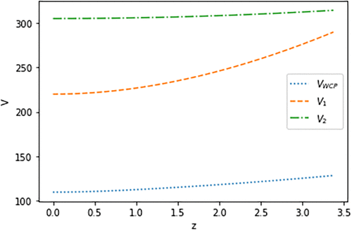
The first numerical results are for the case (A2) introduced in Example 2.7, with . In particular, in Figure 4, we plot three curves: , and . Here, Vi is the cost function for using mode . (The orange/top curve corresponds to V1, and the green/middle curve corresponds to V2.) It is clear from Figure 4 that there is a gap between and both and . We define the “gain” from using the optimal switching policy as
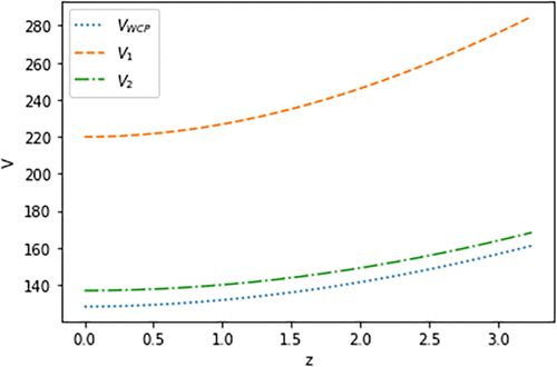
Thus, . For case (A2), G = 1.07. If the cost related to implementing the more complicated switching policy is great enough, it may indeed be decided that G = 1.07 is not sufficient to overcome this cost.
This raises a more general question: Can we place an a priori upper bound on G? It is beyond the scope of this paper to answer this question in any precise mathematical manner, but we provide a set of numerical results suggesting that the answer may be no: Given any , it is possible to find a set of parameters such that G > M. We examine a set of parameters loosely related to case (A2). In particular, we fix and , which are the parameters in case (A2), throughout. We also use . We then take six different values for b1 and set so that
In particular, we take the b1 values to be . Table 2 contains the results of this numerical experiment. Note that G = 1.26 when and grows to G = 5.01 when .
|
Table 2. Gain from Using Switching Policy
| b1 | G | VWCP | ||
|---|---|---|---|---|
| 45/49 | 1.91 | 1.26 | 174 | |
| 90/49 | 1.49 | 1.56 | 141 | |
| 180/49 | 1.13 | 2.01 | 109 | |
| 360/49 | 0.84 | 2.67 | 82 | |
| 720/49 | 0.61 | 3.63 | 61 | |
| 1,440/49 | 0.44 | 5.01 | 44 |
In a very real sense, the situation presented in Figure 4 is a “lucky” one for a system controller who does not want to go through the trouble of implementing the switching policy because the loss is only 7%. The results of Table 2 stand in contrast to that. To see this in graphical form, in Figure 5, we present the same plot as in Figure 4, but corresponding to the parameters in the third row of Table 2. (In this case, V1 and V2 have switched places: The green/top curve corresponds to V2, and the orange/middle curve corresponds to V1.)
3. The LP Under the EHTC
In this section, we prove Lemma 2.1. In addition, in a sequence of three lemmas, we provide an explicit solution to the LP and a criterion for determining whether the two modes are class-switched or server-switched. Finally, Theorem 2.4 is proved. The section is structured as follows. In Section 3.1, we first prove Lemma 2.1(1–3), based mostly on results from Atar et al. (2024). Then, we state Lemmas 3.1 and 3.2, which provide the LP solution, and Lemma 3.3, which is concerned with how the modes are paired. Lemma 2.1(4) is then proved based on Lemma 3.3. In Section 3.2, we prove Lemmas 3.1–3.3 and Theorem 2.4.
3.1. LP-Related Lemmas
Let . It is impossible that for both k = 1 and 2, as this contradicts the EHTC . Assume, then, that, say, . Then, . Define
where . Then, for small, satisfies (2.7) with , which again contradicts the EHTC. This proves Part 1.This follows from Atar et al. (2024, lemma 2.4(4)). Note that uniqueness of the dual problem, which is a standing assumption in Atar et al. (2024), is not used in the proof of this statement.
This statement follows from Atar et al. (2024, lemma 2.3(1)) and Atar et al. (2024, lemma 2.4(4)), where, again, the uniqueness of the dual is not used. □
The following lemma computes the two modes.
Let the EHTCM hold. Then,
The two modes and can be expressed by (3.2) with ξ11 given by
Recall that under the nondegeneracy condition, for any mode, there is a unique relabeling of classes and servers, which transforms it to a canonical form. The following result shows that both modes, once put in canonical form, are given by the same formula.
Let Assumption 2.2 (EHTCM and nondegeneracy) hold. Fix . Relabel classes and servers so that is in canonical form. Then, and
In particular, if and there are i, k such that , then .
Lemma 2.1(4), which is yet to be proved, states that under the nondegeneracy condition, the two modes must be either class- or server-switched. The following lemma contains this result and, in addition, provides a criterion for distinguishing between these cases. We will say that the class-switching condition holds if
Let Assumption 2.2 hold. Then, both modes are nondegenerate. Moreover, under the Class-Switching Condition (3.5), the modes are class-switched (as, for example, in Figure 1, (a) and (b)), and under the Server-Switching Condition (3.6), they are server-switched (as, for example, in Figure 1, (a) and (c)).
The statement is contained in Lemma 3.3. □
Note that cases 2(c) and 2(d) of Theorem 2.13 correspond to class-switched modes (for example, under case 2(c), one has ; hence, the nonbasic activity must have switched from class p to class q when moving from ξL to ξH). By Lemma 3.3, this occurs under (3.5). Also note that in both cases, the proposed policies apply a different rule for the lower and upper workload modes. On the other hand, cases 2(a) and 2(b) of Theorem 2.13 correspond to server-switching and hold under (3.6), and our policies are such that the same rule is used for the lower and upper workload modes.
3.2. Proof of Lemmas 3.1–3.3 and Theorem 2.4
In view of Lemma 2.1(1), every solution ξ is column-stochastic, and, recalling , must satisfy
Identity (3.1) follows.
Next, because the Expression (3.2) is also column-stochastic, proving that any solution ξ is determined by ξ11 as in (3.2) amounts to proving that ξ12 is given as in (3.2). This follows from the first line in (3.7).
It remains to prove (3.3). By the expression just obtained for ξ12, it follows that as long as
Moreover, setting ξ11 to each of the two endpoints of the interval indicated in (3.8) and letting ξ be the corresponding expression from (3.2) gives rise to a solution satisfying all of (3.7), as can be checked directly. Because by (3.2) a solution ξ is an affine function of its entry ξ11, these two endpoints correspond to the two extreme points of ; that is, to the two modes . This proves the lemma. □
Note that Relations (3.7) are invariant to relabeling of classes and servers. Hence, so is Relation (3.2), which was derived solely from (3.7). Let m be given and assume a relabeling has been performed to put in canonical form. Then, satisfies (3.2) with its first column given by . Consequently . Substituting into (3.2) proves (3.4). Because under the nondegeneracy assumption, there can be only one zero entry, in (3.4), we have . Hence, . The final assertion follows from (3.4) using, again, the fact that there can be at most one zero entry □
The four possible graphs and their relabelings are described in Figure 6. Namely, if is the nonbasic activity in , then defining
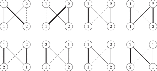
is obtained from upon relabeling in the form of an “N.”
The nondegeneracy of both modes follows from Lemma 3.2.
Next, let the Class-Switching Condition (3.5) hold. Because of (3.1),
Recall from the proof of Lemma 3.1 that the two endpoints of the interval defined in (3.8) correspond to the two modes. Consider the right endpoint. If the minimum in expression in (3.8) is one, then, by (3.2), the nonbasic activity in that mode is (2, 1), and, moreover, . By (3.1), this gives In view of (3.9), this gives
Hence, the maximum in (3.8) is zero. By (3.2), this shows that the nonbasic activity in the other mode is (1, 1). If, on the other hand, the minimum in (3.8) is , then , and the nonbasic activity in the corresponding mode is (1, 2). Similarly, by (3.9),
This means the maximum in (3.8) is not zero. The nonbasic activity in the other mode is then (2, 2). In both cases, the two modes form a class-switched pair as claimed.
Consider now the Server-Switching Condition (3.6). Because of (3.1),
If the minimum in (3.8) is one, then and the nonbasic activity in one mode is (2, 1). By (3.10), . Hence, the maximum in (3.8) is not zero, and the nonbasic activity in the other mode is (2, 2). Finally, if the minimum in (3.8) is not one, then , and the nonbasic activity in one mode is (1, 2). By (3.10), . Hence, the maximum in (3.8) is zero and the nonbasic activity in the other mode is (1, 1). In both cases, the two of modes forms a server-switched pair. □
This lower bound is precisely the one stated in Atar et al. (2024, theorem 2.6), when specialized to the 2 × 2 PSS. To prove that it is valid, we must verify that the standing assumption of Atar et al. (2024), namely, Atar et al. (2024, assumption 2.2), holds.
First, Atar et al. (2024, assumption 2.2.1), which states that the EHTC holds, is valid because of our Assumption 2.2.1. Next, Atar et al. (2024, assumption 2.2.2), when translated to the notation of this paper, states that every is column-stochastic. This holds by our Lemma 2.1.1. It remains to show that Atar et al. (2024, assumption 2.2.3), which states that the dual of (2.7) has a unique solution, is satisfied.
To this end, we shall adopt in the remainder of this proof some notation and terminology from Atar et al. (2024). By Lemma 3.2, the nonbasic activity is different in both modes , for else one would have , contradicting the EHTCM. As a result, with the terminology introduced in Atar et al. (2024, section 2), all the activities are potentially basic. Using strict complementary slackness ((36) in Schrijver 1986, chapter 7) in the same way as in Atar et al. (2024, lemma 2.3.4), any (y, z) solution of the dual satisfies
It follows that . By positivity of both zk, this gives z1 = cz2 for some constant c > 0. Moreover, one of the constraints of the dual problem Atar et al. (2024, equation (2.8)) is . Therefore, are uniquely determined. As a consequence, so are , which shows that the dual problem has at most one solution. The existence of a dual solution follows from the EHTC, as shown in Atar et al. (2024, lemma 2.4.2). This completes the verification of Atar et al. (2024, assumption 2.2). □
4. The WCP and HJB Equation
In this section, Proposition 2.6 is proved. Lemma 4.1, which is used to prove it, contains two additional results: An identification of optimal control systems for the WCP, and weak uniqueness of solutions to the SDE (2.27), both needed for the weak convergence proofs in Section 5.
This is a special case of Atar et al. (2024, proposition 2.5). We comment that the fact that is a classical solution to (2.18) and (2.19) has been established already in Sheng (1978). However, uniqueness of solutions is not covered there. □
In what follows, u always denotes the unique solution to (2.18) and (2.19).
In the following lemma, parts 1 and 2 are largely based on results from Sheng (1978). For completeness, we have included details on the construction from Sheng (1978) (as corrected in Sheng 1981) in Appendix B.
(Optimality in the single-mode case). Assume (2.20) and recall that in this case for m as in (2.20). Then, with u as above, Equation (2.22) of Proposition 2.6 holds. Moreover, for the admissible control system , where is the RBM from (2.26) (assumed to be constructed on the original probability space), and .
(Optimality in the dual-mode case). Assume (2.21) and recall that in this case . Then, there exists a switching point such that (2.23) of Proposition 2.6 holds. Moreover, SDE (2.27) possesses a weak solution . Furthermore, one has for the admissible control system defined by , where .
Weak uniqueness holds for solutions to SDE (2.27).
These results are contained in parts 1 and 2 of Lemma 4.1. □
For Markov control problems, a map from the state space to the control action space is often called a stationary (feedback) control policy, or a policy for short. For our WCP, a policy is thus a measurable map . This term is used in Sheng (1978), and we adopt it in the next proof. Parts 1 and 2 take full advantage of several results from Sheng (1978), where a classical solution to Equations (2.18)–(2.19) is constructed, and a description of an optimal policy is provided.
The Single-Mode Condition (2.20) corresponds to Sheng (1978, section 5.3, equations (41) and (42)). The Dual-Mode Condition (2.21) corresponds to the complementary case. It is stated in Sheng (1978, theorem 1, chapter 4) that a policy is optimal if and only if the cost associated to it is C2 and satisfies Sheng (1978, equation (14), chapter 4), which is the HJB Equation (2.18)–(2.19) in our notation. However, the equation studied there is more general, and in order to reduce it to our (2.18)–(2.19), one must take the switching costs to vanish (by setting the expression K = 0) and the reflection-absorption parameter to correspond to reflection only (by setting λ = 1).
Under the single-mode condition, the policy constructed has the simple form
As for part 2, the claim that the SDE (2.27) possesses a weak solution is proved in Atar et al. (2024, lemma 4.1). Under the dual-mode case, the policy constructed in Sheng (1978) is
We slightly simplify the notation by writing (2.27)–(2.28) as
In the remainder of this proof, and are written as a and b. Let be the operator
Define the operators and in the following way:
The martingale problem for is well posed (for instance by corollary 8.1.2, theorem 4.4.1, and proposition 4.3.1 of Ethier and Kurtz 1986). Therefore, for every probability distribution ν on , there exists a unique solution of the stopped martingale problem for by theorem 4.6.1 of Ethier and Kurtz (1986). Because, for every ,
Next, the martingale problem for is well posed by exercise 7.3.3 of Stroock and Varadhan (2006) (it is shown there that the martingale problem for is well posed, but every solution of the martingale problem for has paths in almost surely). Therefore, for every probability distribution ν on , there exists a unique solution of the stopped martingale problem for by theorem 4.6.1 of Ethier and Kurtz (1986). Because for every there exists such that
Now, one can apply theorem 4.6.2 in Ethier and Kurtz (1986) with for , to conclude that, for every probability distribution ν on , the solution of the martingale problem for is unique.
Finally, because, as already mentioned, every solution to the SDE is a solution to the martingale problem, the weak uniqueness of solutions to the SDE follows. □
(
As it turns out, each of the above three conditions is sufficient for (2.20). This is proved in Lemma C.1 in Appendix C. As a result, each of these conditions is sufficient for nonswitching. These conditions can arise naturally and occur in certain cases in the literature.
5. Asymptotic Optimality
In this section, we prove Theorem 2.13. Toward this, an important intermediate goal is to establish a weak convergence result, stated in Theorem 5.1. The proofs of both theorems rely on four main steps stated in Propositions 5.3–5.6.
5.1. Weak Convergence
5.1.1. Statement of Weak Convergence Result.
We will adopt the following convention regarding the six cases listed in Theorem 2.13. When a statement is said to hold in a certain case of Theorem 2.13, it is meant that the assumptions, as well as the policy, specified in this case are in force. For example, saying that a certain statement holds in case 1(a) of Theorem 2.13 means that it holds when the Single-Mode Condition (2.20) and the condition hold and the P policy is applied, and, moreover, the weaker moment assumption is assumed (but in case 1(b), for example). When a claim is stated without specifying a case, it is meant that it holds in each one of the six.
In addition to the rescaled processes already defined, the weak convergence results will be concerned with additional rescaled processes, namely,
With this notation, the Balance Equation (2.3) for Xn translates under scaling to
Thus, if we denote
The convergence of the rescaled primitives is a direct consequence of the central limit theorem for renewal processes (Billingsley 1999, section 17). Namely, the tuple converges to what we denote by , comprising six mutually independent BMs with zero drift and diffusivity given by the constants and , which in Section 2.3, we have denoted by and , respectively.
Let the assumptions of Theorem 2.13 hold. Then, , where the latter is defined as follows.
In cases 1, (a) and (b) of Theorem 2.13, (W, L) is the RBM and boundary term given by (2.26) and initial condition z = 0, and for all t.
In cases 2, (a)–(d) of Theorem 2.13, (W, L) is the (unique in law) weak solution to the SDE (2.27) with initial condition z = 0, and letting , one has for .
In all cases, Xp = 0 and .
The significance of this result is that it implies that, under each of the proposed policies, limits of the processes exist and form admissible control systems for the WCP, which are, in view of Lemmas 4.1.1–2, optimal.
We next present a lemma from Atar et al. (2024) concerning limits of under general sequences of policies. The Skorohod map, , takes a function ψ to a pair , where
The corresponding maps and are denoted by and , respectively.
Let be any sequence of admissible controls for the QCP for which . Then, the following conclusions hold. The sequence is C-tight. Along any convergent subsequence where , one has
This is the content of Atar et al. (2024, lemmas 5.1 and 5.5). □
This lemma is our starting point for proving Theorem 5.1. Whereas it relates limits of processes associated with the QCP to an admissible control system for the WCP, note that it does not make any claim regarding or and, hence, by itself is not sufficient to relate the prelimit cost (defined in terms of ) to the WCP cost. In particular, the pair need not be the weak limit of . To proceed, one must show that under the proposed policies, along the sequence specified in Lemma 5.2, one has
The propositions presented below address these issues as follows. Proposition 5.3 provides uniform integrability required to eventually deduce Theorem 2.13 from Theorem 5.1 and, in addition, ensures that the prelimit cost remains bounded so Lemma 5.2 may be applied. Proposition 5.4 shows that in probability. Proposition 5.5 states precisely what is needed to attain (5.9). Finally, Proposition 5.6 implies that (2.27) holds in the dual-mode case.
5.1.2. Main Steps Toward Weak Convergence.
Throughout what follows, the assumptions of Theorem 2.13 are in force. The four main steps required to achieve weak convergence and, later, Theorem 2.13, are as follows.
There exists such that
As already mentioned, this uniform integrability result will allow us to deduce convergence of the costs, as stated in Theorem 2.13, from the convergence stated in Theorem 5.1. Moreover, because it also implies boundedness of the cost under the proposed policies, it enables us to use Lemma 5.2. The proof is given in Section 5.2.2.
For every , as ,
The above type of result is often referred to as state-space collapse (SSC), as it asserts that, asymptotically, all workload is kept in one buffer, a property crucially used in establishing the one-dimensional state space description of the limiting dynamics, as well as asymptotic optimality, because all workload is held in the “less expensive” class. It is proved in Section 5.2.3.
Consider a subsequence as in Lemma 5.2, where . Then, along this sequence, one has , where F is given by (5.8), and . In particular, is a C-tight sequence, and the conclusions of Lemma 5.2 hold with .
The proof appears in Sections 5.2.4 and 5.2.5.
Finally, the policies P and that are proposed under the single-mode condition do not use the nonbasic activity of the active mode ξA. For the four policies employed under the dual-mode condition, we need the following control over the use of the nonbasic activities corresponding to ξL and ξH.
Consider the same subsequence as in Proposition 5.5 and cases 2(a)–(d) of Theorem 2.13. If (resp. ) denotes the nonbasic activity in ξL (resp. ξH), then for any and ,
To explain the role of this proposition, recall that if , then the condition for some activity (i, k) not only implies that ξ is one is the modes or , but also identifies which one by Lemma 3.2. Because any limit T of Tn is given as , this proposition implies that when workload is either below or above the switching point, the resource allocation asymptotically follows the respective mode of operation ξL or ξH. This is very close to stating that the pair (W, L) follows the SDE (2.27) and, indeed, is the basis for proving this fact. The proof of this proposition appears in Section 5.2.6.
5.1.3. Considerations for the Construction of Dual-Mode Policies.
As noted above, two of the key results that we need to prove Theorem 2.13 are state-space collapse (Proposition 5.4) and a boundary property stating that there is asymptotically no idleness of either server when there is work in the system (Proposition 5.5). The proofs of these results differ by case/policy and, for dual-mode policies, rely on the rules used as well as the way that workload is sampled. Here, we provide a brief description of the reasons underlying the policy definitions that we have used.
A difficulty arises in the proof of Proposition 5.4 in case 2(a), where the policy switches between two P rules. Only the dual-activity server in the current mode processes the HPC and the identity of the dual-activity server changes when switching modes. At each switching time, if the server processing the HPC in the new mode is busy with low-priority jobs and the service of the high-priority job at the other server ends, no server will process high-priority jobs for a time . In principle, this time could accumulate to let the number of high-priority jobs increase to a nonnegligible value. In order to prevent this, we designed switching between P rules to only occur at the time of service completion at the single-activity server. When switching, this server becomes dual activity and gives priority to the HPC (which is the single-activity class in P). In case 2(a), there is always at least one server processing the HPC, regardless of switching between modes.
Similarly, in order to prove Proposition 5.5 in case 2(b), we need to show that the number of HPC is not zero when there are low-priority jobs in the system. To make sure that the high-priority class does not receive too much service, switching between two rules only occurs at the time of service completion at the single-activity server. When switching, the single-activity server becomes dual activity and now gives priority to the low-priority jobs if the number of HPC jobs is low. In case 2(b), as long as the number of HPC jobs is below the threshold there is at most one server working on HPC jobs, regardless of switching between modes.
In case 2(c), it should be noted that in the lower mode, the system looks similar to case 1(a), so one could consider using a P rule. Doing so, however, would cause difficulty in proving Proposition 5.5 for this case. Using a P rule keeps the number of HPC jobs O(1). At the moment of switching into the rule, this can lead to the new single-activity server, which is dedicated to HPC, incurring idle time when there is work in the system. To avoid this situation, the rule was used instead of P, guaranteeing that, at a switching time, there will not be too few HPC jobs in the system. A similar argument applies to case 2(d).
5.1.4. Proof of Weak Convergence.
Here, we prove Theorem 5.1 based on the four propositions.
First, by Proposition 5.3, one has that for each one of the relevant policies Tn. As a result, the assumptions of Lemma 5.2 and Proposition 5.5 are valid. To summarize the conclusions from these results, fix a subsequence along which . Then, there exists a tuple such that, along this sequence,
Next, by Proposition 5.4, in probability. Also, by (2.11), , and, therefore, we now have, along the subsequence, , where we denote
Note that the control system thus constructed may depend on the subsequence. However, consider the following.
In case 1, (a)–(b) of Theorem 2.13, (W, L) is the RBM, and its boundary term given by (2.26), and for all t. In cases 2(a)–(d) of Theorem 2.13, (W, L) is a weak solution to the SDE (2.27), and, moreover, for a.e. t.
Suppose the above claim holds true. Then, the law of (W, L) is uniquely determined: in case 1 as an RBM; in case 2 as a weak solution to (2.27), for which weak uniqueness holds by Lemma 4.1.3. In particular, this law does not depend on the subsequence. Moreover, because by this claim and (5.12), the pair of processes (T, X) is uniquely determined by W (away from a -null set), it follows that the law of does not depend on the subsequence. This yields the convergence along the full sequence and completes the proof of the result. In what follows, the claim is proved.
Consider first the single-mode case, namely, cases 1(a)–(b) of Theorem 2.13. The policies employed are P and , and both do not use the nonbasic activity of the active mode ξA. In other words, if we denote this activity by , then under these policies, for all n. As a consequence, the limit process T must satisfy a.s.; hence, for a.e. t, a.s. By the uniqueness statement made in Lemma 3.2, whenever and , one must have . It follows that for a.e. t, and, hence . As a consequence, (5.11) holds as . That is, the pair (W, L) satisfies (2.26). This proves the first part of the claim.
Next, consider the dual mode, namely, cases 2(a)–(d) of Theorem 2.13. First, we will show based on Proposition 5.6 that, for every and ,
By the continuous mapping theorem, we have along the subsequence . In addition, Tn is continuous with finite variation over compacts. By theorem 2.2 of Kurtz and Protter (1991),
By Proposition 5.6, in probability. Hence, the left-hand side (LHS) in (5.15) converges to zero in probability. Thus, the RHS in (5.15) equals zero a.s., and, therefore, by the first inequality in (5.14), the first part of (5.13) is proved. The second part of (5.13) is proved analogously.
Next, clearly, . Hence, by (5.13), . Arguing, again, by the uniqueness statement in Lemma 3.2, one has whenever . It follows that, a.s.,
Notice that Ut does not depend on ε, so if we manage to prove that the RHS converges to zero in probability as , it follows that, for every t, Ut = 0 a.s. Hence, by continuity of this process, Ut = 0 for all t, a.s. That is, the processes (W, L, B) satisfy (2.27) a.s.
To this end, apply the occupation times formula (Revuz and Yor 1999, corollary VI.1.6), by which for any continuous semimartingale Y, one has, a.s.,
Next, for the stochastic integral , we have
By local boundedness of and its a.s. convergence to 0 as , it follows that in probability. A similar argument holds for . We conclude that (W, L, B) satisfies (2.27). Finally, by (5.16) and the fact a.s. just proved, one has for a.e. t, a.s., which completes the proof of the claim, and also of the result. □
5.1.5. Proof of Theorem 2.13 and Corollary 2.15.
As a consequence of Theorem 5.1 and Proposition 5.3, we have the following.
The weak convergence statements asserted in the theorem are already established in Theorem 5.1. For the AO results, we need to show that in each of the six cases . Combining Theorem 5.1 with the identification of an optimal control for the WCP given in Lemma 4.1 shows that , where Xp = 0 and , W is given by (2.26) or (2.27) in the respective cases, and, moreover,
The convergence stated above implies
By (2.6), . Hence, the convergence will follow from (5.17) once uniform integrability is established. Arguing along the lines of Bell and Williams (2001, pp. 640–643), introduce the measure on and invoke the Skorohod representation theorem to obtain from (5.17) that -a.e. Accordingly, uniform integrability of Hn w.r.t. suffices to obtain . However, this is ensured by Proposition 5.3, for
As far as the proof of the Weak Convergence (2.29) and AO are concerned, there is no difference between the setting of Theorem 2.13(1), where the LP has multiple solutions but the single-mode condition holds, and the case where it has a single solution. Therefore, this result is a corollary of Theorem 2.13(1). □
5.2. Proof of Propositions 5.3–5.6
In Section 5.2.1, we provide several useful estimates. Then, Propositions 5.3, 5.4, 5.5, and 5.6 are proved in Section 5.2.2, Section 5.2.3, Sections 5.2.4 and 5.2.5, and Section 5.2.6, respectively.
5.2.1. Auxiliary Lemmas.
Two estimates on the rescaled primitives, and , are provided in (5.18) and Lemma 5.7, and a certain estimate on the maximum service duration is given in Lemma 5.9.
Because the assumptions on and are similar, the estimates are stated for , but apply also for . Recall that are interarrival times of Ai and thus are the interarrival times of . Recall for a constant . The first estimate is Krichagina and Taksar (1992, theorem 4), which states that for any ,
Let be such that and assume that (note, in particular, that for every , there exists satisfying these conditions). Fix . Then, for any ,
The proof appears in Appendix A.
We sometimes use the balance equation in the following form, which follows from (5.4), namely,
Note that of (5.5) is given by Then, using the 1-Lipschitz property of the trajectories of , it is easy to see that both estimates above imply some estimates for . In particular, by (5.18), . Moreover, under the assumptions of Lemma 5.7 and the additional assumption that , the conclusion of the lemma holds for and .
Next, we give an estimate on the maximal service duration and interarrival time up to a given time. The time in service by t of a given job is defined as the time that the job has spent in service up to time t. Let denote the time in service by t of the lth job in activity (i, k). If service to job l has completed by time t, then, clearly, , but if it is still in service, . Of course, for jobs for which service has not started by t. For t > 0 and a real-valued path , denote
Then, for activity (i, k), the maximal time in service by time t, namely, , is bounded above by . We will need an upper bound on the service time as well as the interarrival times, and to this end define
This process also bounds from above all service durations completed by time t.
One has for a constant c that does not depend on n or t. Moreover, for any and , as .
The proof appears in Appendix A.
5.2.2. Uniform Integrability.
Here, we prove Proposition 5.3. We sometimes need to refer to the variable keeping track of the current mode, which in the various policies is defined in slightly different ways according to different sampling times. Denote
The proof has three parts; part 1 appears below, while parts 2 and 3 are deferred to Appendix A. Fix any one of the sequences of policies for which we attempt to prove AO.
Part 1. This part is concerned with the case where, whenever the workload in the system is sufficiently large, policy P is active. This covers case 1(a) of Theorem 2.13, where the system has a single mode and the fixed priority policy P is applied, as well as case 2(a), where the dual-mode policy PP is applied. In this case, we will prove that the statement of the lemma holds with , and specifically that, under the given sequence, is bounded by a polynomial in t for all n. By (2.11), this is equivalent to the same property holding for .
To prove the result in this case, assume that in the single (resp., dual)-mode case, the active mode ξA (resp., the high-workload mode ξH) is in canonical form. Thus, provided that the workload in the system exceeds (when applicable), class 1 (resp., 2) is the dual (single)-activity class, and server 1 (resp., 2) is the single (dual)-activity server. In addition, p = 2: class 2 is the HPC. First, we provide a bound on the second moment of . In the dual-mode case, fix K large enough so that implies ; in the single-mode case let K = 1. Given t > 0, consider the event . Let be defined by
Because the system starts empty, , and because the jumps of the normalized queue length are of size . Thus,
By (5.3), denoting ,
Because in , the priority policy corresponding to a mode given in canonical form (either ξA or ξH) is in force after an initial time before the current mode updates and there are class 2 jobs to serve. We can bound the time until server 2 prioritizes class 2 and starts serving it at full rate in by . If there currently is a class 2 job being served by server 2, server 2 only serves class 2 jobs for the whole period and
If there currently is a class 1 job being served by server 2, because service is nonpreemptive, server 2 has to finish this job. If at that time, the current mode is ξH (resp. ξA in the single-mode case), server 2 prioritizes class 2 from that point on. If at that time, the current mode is ξL, the workload is then sampled because a service finished at the single activity server. The current mode changes to ξH and stays until t. In both cases, we get
Also, in the case under consideration, one has . Hence, for all sufficiently large n, . Moreover, . Hence,
The above inequality holds also on the complementary event, namely, when . Thus, using (5.18) and Lemma 5.9, we obtain
In the next step, we bound . Let be a constant that is sufficiently large to ensure that implies (where, again, in the single-mode case). Given t > 0, consider the event and let be
Then, clearly, . Because during , there are at least two jobs of class 1 in the system, both servers are never idle during . Because one has , it follows that . Hence,
By (5.6) and the nonidling of both servers during , by which remains flat during this interval, we have . Thus, by (5.5), for a constant c (that may depend on ),
Clearly, the above bound is valid also in the complementary event, . We can therefore apply (5.18) and (5.21), to obtain for some constant c, for all n and t. Consequently, the same holds for the second moment of , and the result follows. This completes part 1 of the proof. The remaining parts appear in Appendix A. □
5.2.3. State Space Collapse.
We now prove Proposition 5.4. Assume that either the active mode ξA or the lower workload mode ξL (whichever is applicable) is in canonical form. Let
This random time is used outside this proof with the notation , but in this proof, the shorter notation τ is used. Then,
We will prove the lemma by showing that the RHS above converges to zero as . On the event , define
The proof relies on the fact that, under our policies, when the number of HPC jobs is above , it is served at a rate that is enough to deplete the queue in all cases. The first step toward this goal is the following.
There exist constants such that, on ,
First, by definition of σ, and τ, and the fact that jumps of are of size for large n, we obtain
We address here one case only; the proof under the remaining cases is deferred to Appendix A.
Case 1(a): In this case, we use the P policy, which is single mode. Because the active mode is in canonical form and , p = 2, and server 2 prioritizes class 2. It is possible that server 2 is busy with the “wrong” class of job at time σ, but as soon as that job finishes, server 2 will only serve the class 2 jobs in the system:
Thus,
To show that , note that since the active mode is in canonical form, , which implies by (3.1).
The remaining cases appear in Appendix A. □
Now that Lemma 5.10 has been proved in all cases, the proof of Proposition 5.4 does not need to differentiate between them.
Let and . Recall that , as defined in (2.32), so that . Notice that, as required in Lemma 5.7, . Let us introduce the event
For n large enough, one has . Consequently, . We obtain
Picking up on (5.19), by Lemma 5.10
Notice that on the event ,
Thus,
Recall that , so . By Lemma 5.7 and Remark 5.8, the first term converges to zero. By Lemma 5.9 and ,
For the second term in (5.23), notice that on ,
Hence,
By Lemma 5.9, is smaller than . By Remark 5.8, is a tight sequence of random variables (RVs) (for t0 fixed). Because . The claim follows. □
5.2.4. Boundary Behavior.
The goal of this section and the following one is to prove Proposition 5.5. The key is the following lemma, which states, roughly speaking, that is approximately the boundary term corresponding to .
Let .
Fix . With
in probability as .
This lemma is proved in the next subsection. Let us show how Proposition 5.5 now follows.
In addition to just introduced, we shall need the following definitions:
By (5.6) and definition of the new processes, one has
Consider the pair . The first component is nonnegative. The second is nonnegative, nondecreasing, and, moreover,
Hence, by Skorohod’s Lemma, . Hence,
Recall that we are considering a subsequence along which (according to the assumptions and to Lemma 5.2), , with F as in (5.8). Moreover, by the definition of Zn and , we have , whereas by Lemma 5.11, in probability. By the continuity of the map , we therefore conclude from (5.25) that, on the same subsequence,
5.2.5. Proof of Lemma 5.11.
We first explain how the proof changes between the cases.
Under the P policy, both servers can process the low priority jobs. This means that idling can only occur if the low-priority class has few jobs, and, in that case, the total number of jobs is also low by Proposition 5.4.
Under the rule, no server can incur idleness when the high-priority class is above the threshold. In addition, the high-priority class takes a small time to reach above and does not empty below two jobs after that time with high probability unless the total workload is close to zero (Lemma 5.13). This means that neither server will idle except when there are almost no jobs in the system.
Under the PP policy, Proposition 5.4 is still enough to prove Lemma 5.11 in the same way as in the single-mode case P.
Under the policy, Lemma 5.12 and 5.13 hold. Because of that, Lemma 5.11 holds for the same reason as in the nonswitching case .
When using a P rule, the high-priority class could become zero with a lot of LPC jobs in the system, and switching to the rule could lead to idleness, even though there are a lot of low-priority jobs (approximately ). Thus, we introduce the rule in place of the P rule in this case. This ensures that the number of high-priority jobs does not decrease too much during the corresponding period.
In some cases, some idleness can occur when the high-priority class starts with too few jobs, but in those cases, it takes a small time to leave such states.
In cases 1(a) and 2(a), Lemma 5.11 is a direct consequence of the state space collapse. Let us introduce two random times and a lemma that we will use in cases 1(b) and 2(b)–(d). Fix . Let
If any of the following conditions hold, we have
Under the same assumptions as the previous lemma,
The proofs of Lemmas 5.12 and 5.13 appear in Appendix A.
The above two lemmas do not address cases 1(a) and 2(a). The reason for this is that in these cases, we can directly prove Lemma 5.11 when using a P or PP policy.
Here, we only treat one case, deferring the remaining cases to Appendix A.
Case 1(a), P policy:
In this case, p = 2, and no server can be idle when . Thus,
For any ,
By Proposition 5.4,
The treatment of the remaining cases appears in Appendix A. □
5.2.6. Fast Switching
Fix t0 and . Assume that ξL is in canonical form. Then, . Let
If , the current mode never changes, so the single-activity server is dedicated to only one class for the whole period and the nonbasic activity is never used. Thus,
Note that we have used the fact that, for all of our policies, jobs are never routed to a nonbasic activity of the current mode.
The remainder of the argument is based on the following fact, which must be argued separately for each case. This is concerned with the difference , which, although case-dependent, can in all cases be shown to satisfy
By Proposition 5.5, is C-tight. Hence, for any constant c > 0, . On the other hand, by Lemma 5.9, . Thus,
In order for to become positive, must be smaller than t0 and
It is not possible for to occur on . If that were the case, server 1 would necessarily finish service of the job it was in the process of serving at time τ1 before the workload has time to reach . When in canonical form, server 1 can only take new class 1 jobs, regardless of the rule. Even if class 1 has no job in the queue, the nonbasic activity is not used after the possible residual job that was in service at time τ1. In addition, by definition of , this is the last time the mode switches from upper to lower workload before τf. This would prevent from becoming positive and is also the reason why needs to be smaller than t0 for τf to be smaller than t0.
By definition of and κn,
We next show that
We have
Both terms converge to zero, the first by (5.30) and the second by (5.31).
We can now prove the lemma based on (5.32), (5.30), and (5.31). We have
The first term goes to zero by (5.32), the second by (5.31), the third is zero, and the fourth goes to zero by (5.30). This completes the proof.
It remains to prove (5.30). As noted above, the proof differs by case.
Case 2(a): The current mode changes to ξL after the first service completion of a job at the single-activity server for ξH (which is server 2) at or after . Note that must correspond to a service completion. If corresponds to a service completion at server 2, the . If corresponds to a service completion at server 1, then the mode will not change, and τ1 will correspond to the next service completion at server 2. This will occur before if server 2 is busy (serving class 1) at . Note that, on , so that
Case 2(b): The current mode changes after the first service completion of a job at the single-activity server (which is server 2) at or after . Server 2 is dedicated to HPC jobs. Under , there are at least two HPC jobs in the system at time , so the single-activity server cannot be idling at that time. Thus,
By Lemma 5.13, converges to zero. In addition,
Cases 2(c) and 2(d): The current mode changes after the first service completion or arrival of a low- or high-priority job after so under ,
The authors are grateful to Cristina Costantini for providing us with the proof of Lemma 4.1, part 3, and to two anonymous referees, as well as the anonymous associate editor, for their thoughtful suggestions that helped improve the exposition considerably.
Appendix A. Proofs of Lemmas
In this proof, m is written as m. Note first that it suffices to prove
Moreover, can be made arbitrarily close to h0 by choosing close to ν2. This shows that the desired inequality holds for all large n, and by making larger, for all .
We now prove (A.1). As before, c denotes a positive constant whose value may change from line to line; here it may depend on but not on n, t0. By (5.1),
Thus,
Consider the event . Because are the interarrival times of An, on this event, there must exist and such that
Recall that . Letting , we have . Then, taking , using where , we have
Let , and note that it is a martingale. For a real-valued function X on let
Then, using and denoting ,
Because , we have the lower bound for some c > 0 and all large n. Hence Burkholder’s inequality shows that
Hence, for any a > 0, , and, therefore,
Note that by the assumption . Now, if and a > 0, then, with , . This gives
By a similar argument, the same estimate holds for . An application of (5.18) gives
Hence, by (A.2),
It follows from that . The result follows. □
Fix i, k. Denote . For any u > 0, if , then there must exist with and ; hence, by the Definition (5.1) of ,
To prove the second statement, we will proceed in two steps. First, we will show that the number of interarrival times involved in the maximum is at most cn with probability going to one, then show that the maximum over cn variables has the right order of magnitude.
To simplify the notation, fix (i, k) and remove them from the notation of , etc. The claim will be proved for defined as in (5.20), but without maximizing over (i, k); clearly, this is sufficient. Note that
Let
Then,
For any ,
If , by the law of large numbers, the RHS converges to 0 as . Next, by independence of service times, for any c > 0,
Using , letting and denoting , we obtain
Thus,
Hence, for any c > 0, there exists c2 such that
(
Part 2. Consider the case where is applicable when the workload is sufficiently large. This covers case 2(d) of Theorem 2.13, in which the policy applies (none of our proposed policies implement as a single-mode policy). The proof given in part 1 is applicable, for the following reasons. In the first step, during the analyzed time interval , one has , and, therefore, there is no difference between how P and behave during this interval. In addition, the workload is sampled at each arrival/service, which means that
In the second step, the argument given for nonidling of both servers during again holds here, similarly to part 1, upon noticing that, because σ corresponds to an arrival, it is a sampling time, and so the current mode is either already the high mode or switches to the high mode at that time. (It is possible that, if σ is a mode switching time, then server 1 was idle just before σ. But, if so, it starts to serve class 1 at σ.) The remaining details need no adaptation.
Part 3. Finally, consider the policies that employ for high workload levels, namely, the policies , , and , covering all remaining cases of Theorem 2.13. In these cases, the stronger moment assumption is in force, and the goal is to prove that there exists such that for all n and t, for some polynomial . As before, let ξA or ξH be in canonical form, in the single-mode and, respectively, dual-mode case. Fix a constant in the dual-mode case and K = 1 in the single-mode case. Given t, consider the event . Let
Then, , and, moreover, during . Although this lower bound on the workload is sufficiently large to guarantee that corresponds to the higher workload mode, it is possible that at time τ1, the current mode variable still equals the lower workload mode. We argue that the time it takes to switch to the upper workload mode is bounded by in both and . In the former case, the current mode switches as soon as a there is a new arrival or departure. In the latter case, one possibly has to complete the service of a job at server 2, which is server . It is possible that there are no jobs allowed to be routed to server 2 at time τ1. Wait for an arrival of class 1 job, and service completion of this job at server 2. At this time, it is guaranteed that mode has switched to ξH if it was not ξH earlier. Thus, if we let
According to the rules of , server 2 must be busy throughout the interval . Thus, . Hence, by (5.6), and using (by (5.2)), we have
Hence, it suffices to bound the last term above by a polynomial in t.
To this end, let . Then,
To bound , consider the event . On it, during the interval , one has ; hence, by the rules of , server 2 prioritizes class 2, except possibly it completes a service that started when . Moreover, during the same interval, by which we know that there are multiple class-2 jobs in the system, and, thus, server 2 gives no service to class 1, with the only exception of service to a job that started when . Hence, the departure process associated with activity (1, 2) increases by at most one during this interval that is, . Recalling the definition of in (5.1), this can be expressed as , where
Using this in (5.4) gives, for ,
Next, by (2.4),
However, activity (2, 1) is not in use by . Denoting and , this yields
Because is used after the update of modes, it must be true that .
We use the following property of the Skorohod map. Let . Then, by (5.7), . Assume that where . Then,
This property is used as follows. On the interval , can increase only at times when ; and the latter process is nonnegative. This shows that serves as the Skorohod term in (A.3) on that interval, and, thus, by the non-negativity of and c1, and the bound , this shows that
Hence, .
Next, we bound . To this end, consider the event . Because by its definition, , we have
On the event , let
Then, on , it must hold that . The arguments that led to (A.3) are valid for the time interval . As a result,
Given any , using the nonnegativity of the second term on the LHS, in the case that , one must have . On the other hand, in the case , one must have . As a result,
We have by (2.32) , where we recall that . Thus, by Lemma 5.7, with , one has, for any ,
Next, by (5.18) and Chebychev’s inequality,
As a result, we have
By our assumptions, we have and . Using this, a calculation shows that with the choice , one has . It follows that there exist and for which . Therefore, and the proof is complete. □
(
Case 1(b): In this case, we use the policy, which is single mode. Between σ and τ, . Thus, both servers give priority to the HPC at all time in . It is possible that the dual-activity server is occupied with the low-priority class at σ, but as soon as the current job is served, the high-priority class gets priority on one server and dedication by the other server. By definition of , we have for any ,
Thus,
Finally, by (3.1) and .
Case 2(a): In this case, we use the PP policy, which only changes mode at the completion of a service at the single-activity server. This is precisely the server that gives priority to the high-priority class after switching mode because we are in an SS case. Because there are always HPC jobs to serve between σ and τ, we claim that excluding an initial period, at any given time the HPC is being served by at least one server, as discussed in Section 5.1.3. We now discuss how long this initial period can be.
The only way some service is lost is if there were no high-priority jobs at some point in the system, both servers become busy with low-priority jobs, and σ occurs before the service completion of those jobs. After completion of those two jobs, the HPC keeps priority on at least one server, regardless of switching of the current mode. For the initial jobs, with respect to , either the service ends first at the dual-activity server or the service ends first at the single-activity server.
In the first case, a service of the HPC job starts at the dual-activity server because it has priority there until either τ is reached or a mode switch occurs. In the second case, the available server is currently dedicated to the LPC. Because this corresponds to a service completion at the single-activity server, the workload is sampled, and there could also be a switching of modes. If the mode changes, then this server becomes dual activity, and the HPC has priority there. If there is no mode switch, the service of another LPC job starts. LPC jobs are served at this server until the mode switches.
Thus, if the service ends at the dual-activity server before the mode switches, then an HPC job will start there. If the mode switches before the service ends at the current dual-activity server, then the current single-activity server becomes dual activity and an HPC job begins service there.
In either case, the HPC is served by at least one server after that time because it has priority on the dual-activity server, and the dual-activity server is always available when switching modes. In addition, the time it takes for the HPC to begin service is smaller than the service of the job present at the dual-activity server at time σ, which is smaller than . Hence,
This yields
In addition, . Putting ξL in canonical form forces in this case and p = 2 because . In addition, by (3.6), either or . Thus, , which implies by (3.1).
Case 2(b): In this case, we use the policy. Because the number of HPC jobs stays above throughout the period , both servers only take new jobs from the HPC, regardless of the mode. Similarly to 1(b), there is at most one job served at either activity before the HPC gets served. Hence, for any ,
Thus,
We obtain the result similarly as before because .
Cases 2(c) and 2(d): The HPC is single activity in one mode and dual activity in the other. Recall that this case is CS. This means the dual activity server stays the same, regardless of switching modes. When a rule is applied, the dual-activity server prioritizes the single-activity class as long as there are more than jobs of this class. The HPC is single activity when we apply the rule. Similarly, under a rule, the dual-activity server prioritizes the dual-activity class as long as there are more than jobs of this class and the HPC is dual activity when we apply the rule. Once again, put ξL in canonical form, server 2 is the dual-activity server in both modes. Regardless of which rule is used, as long as the number of HPC jobs is above , server 2 only takes new jobs from the HPC. As before, we have to exclude a residual service of a low-priority job that started before σ. Hence,
It remains to show that the activity processing HPC jobs throughout the period is enough to deplete them. Because of the canonical form of ξL, and, thus, by (3.5), . Moreover, by (3.1). Whichever the HPC is, server 2 has enough capacity to deplete it. In other words, and
The proof follows reasoning similar to the proof of Proposition 5.4. Fix δ. Let us introduce
In cases 2(b), (c), and (d), introduce
To simplify, we write throughout this proof
We briefly describe the interaction between the times we just introduced. Under the state-space collapse, has to occur before the first time the current mode switches. The times σ and allow us to have some knowledge about the state of queue lengths, uniformly over an interval. The first step of the proof of (5.26) is establishing that
In addition, in case 1(b), for any
We now proceed with the proof of (A.4). On , the following hold:
(i) The number of HPC job is below , and there are LPC jobs in the system during :
(ii) The current mode is the same as in the initial state: for any ,
(iii) In addition, the number of LPC jobs must have grown during that time:
(i) comes from the definition of ρ, and . (ii) comes from the fact that the number of HPC jobs is bounded by under and the number of LPC jobs is bounded by before and the workload cannot cross above . (iii) comes from the definition of and . Because of (ii), only the rule in the lower-workload mode is in use. When using a rule, both servers take new jobs from the LPC because of (i), and . When using a rule, again because of (i), the dual-activity server takes new jobs from the LPC. Because ξL is in canonical form and q = 2 because of the rule. This means that and, thus, . Hence, with (5.19), regardless of the case there exists c > 0 such that
From this, we obtain two bounds:
We now prove (A.4): let . Because of (iii),
By Lemma 5.9, is smaller than . By Remark 5.8, are C-tight and are tight RVs. Both terms must then converge to zero. This concludes the proof of (A.4) in all relevant cases for this lemma.
Case 2(c), rule:
By splitting the integral that defines , and using (5.24) and (A.5),
The first term is zero by definition of the rule because q is the dual-activity class. The second term goes to zero by Proposition 5.4 and (A.4). This concludes the proof of (5.26) in case 2(c).
Case 1(b), 2(b), and 2(d), rule:
We now deal with all cases that use a rule in lower workload at the same time thanks to (A.5)/(A.6). Recall that and . By splitting the integral, we obtain
By (5.2), . By definition of the rule, as long as there are at least two customers in the system, the dual-activity server cannot idle. With ξL in canonical form, server 2 is the dual-activity server, so under the event ,
Because by Proposition 5.4, we are left to deal with
We introduce the following times:
andWe want to show that
On the event , we have:
• First, by definition of ,
• Second, by definition of ρ,
• Finally, by definition of ,
In order for server 1 to be idle at time (so that ), it is necessary that . This means that in order to also have , we need to have , or
(A.7)
We can now give the balance equation for between and under the rule. Under the rule, server 2 prioritizes class 2 for the whole period because the number of HPC jobs remains below . Because we obtain from (3.1). By the same reasoning as (A.3), there exists such that
Combining (A.7) and (A.8), we obtain (on )
As in the proof of Proposition 5.4, we distinguish between two cases: smaller or larger than . On , , so that
On and , so that
To summarize,
All terms converge to zero. The first two have already been treated in Proposition 5.4 and (A.4), respectively. The third term converges by Lemma 5.7, the fourth and sixth by Lemma 5.9, and the fifth by tightness of .
This completes the proof of (5.26) and Lemma 5.12 in all of the relevant cases. □
Case 1(b), T2 policy:
We begin the proof by a full analysis in the case where a policy is used and then explain how to deal with the other cases. In this case, with the active mode in canonical form, p = 1. Recall the definition of the random time τ:
andFor any ,
• ,
• and .
In this case, only server 1 processes class 1 jobs and does so at most at full rate. Indeed, only server 1 gives priority to class 1 jobs, and the other server is busy with class 2 jobs present in the system. Similarly, only server 2 processes class 2 jobs and does so at full rate because there are always class 2 jobs and the number of HPC jobs is below between σ and τ. Similarly to Lemma 5.10, is such that for any , including a service that could start before σ at the wrong activity (server 2 in this case),
and excluding a service of a HPC job by server 2 starting before σ,With the active mode in canonical form, we have . By (3.1), this means . Thus, and .
There are two possibilities for the state of the system at time σ: we have either
,
or .
We will decompose the event in two events:
withandTo lighten notation, introduce also
Similarly to Proposition 5.4, let and so that . Then,
On , we also have
On the event , the reasoning is very similar to the proof of Proposition 5.4:
(A.9)The last probability goes to zero by tightness of and Lemma 5.9. When the situation is again the same as in the proof of Proposition 5.4:
(A.10)The right-hand side also converges to zero by Lemma 5.7, Remark 5.8, and Lemma 5.9, similarly to the proof of Proposition 5.4.
The second event is treated similarly:
On this event, we also have
On the event , similar to the treatment of :
(A.11)The last probability goes to zero by tightness of and Lemma 5.9. When , the situation is also the same as for :
(A.12)The right-hand side also converges to zero by Lemma 5.7, similarly to the case. This concludes the proof in case 1(b). We now present the changes required to adapt the proof to the other cases described in the lemma:
Case 2(b), policy:
This case involves switching between two rules: . Because ξL is in canonical form, p = 1. In this case, mode switching only occurs at a service completion at the single-activity server that is dedicated to HPC jobs. There could be either type of job being served at either server immediately before time σ. We will see that after those jobs exit the system, there is at least one server processing the LPC and at most one processing the HPC. If the first job to finish is from the dual-activity server, the service of a low-priority job starts because there are fewer than HPC jobs. This server will continue to take LPC jobs until the minimum between the next mode switching time and τ. If the first job to finish at or after σ is at the single-activity server, either the current mode switches or the service of an HPC job starts. If there is no mode switch, then this server will continue to take HPC jobs until the minimum between the next mode switching time and τ. When the dual-activity server completes its job, it will, as noted before, serve LPC jobs. If there is a mode switch, then the formerly single-activity server becomes dual activity, and (because there are fewer than HPC jobs) begins service on an LPC job. When the formerly dual-activity server completes its job, it becomes single activity and serves HPC. This continues until the minimum between the next mode switching time and τ.
After the two jobs present at σ, there cannot be a time where both servers are occupied with HPC jobs. This is because the HPC is only processed by the server dedicated to it, and there can be no residual service of an HPC job at the single activity server whenever the current mode switches. Similarly, after both initial jobs have been processed, there is always at least one server occupied with LPC jobs. This is because one server gives priority to the LPC, and the service of a LPC job starts whenever the current mode switches.
Keeping the definition of τ, σ, just as in the single-mode case, for any , including/excluding a service that could start before σ at the wrong activity, there is always at most one server processing HPC jobs and at least one server processing LPC jobs between σ and τ. Thus,
andWith one mode in canonical form we have . In addition, by Lemma 3.3, in case 2(b), (3.6) holds, and, thus, , which also means by (3.1).
The rest of the proof is the same as in the single-mode case, obtaining (A.9), (A.10), (A.11), and (A.12). This concludes the proof in case 2(b).
Case 2(c), T1T2 policy:
With ξL in canonical form, we have p = 2, so τ and σ are defined as
andIn this case, in the upper-workload mode, only the single-activity server is allowed to begin service of the HPC between σ and τ, whereas in the lower-workload mode, neither server can begin service of HPC between σ and τ. Between those times, there are always low-priority class jobs to serve, and the number of HPC jobs stays below . The most service the HPC can get between σ and τ occurs if there are no switches and the current mode is always upper workload. In this mode, the single-activity server (server 1) is dedicated to service of the HPC. Hence, including a service that could start before σ at the wrong activity,
Between σ and τ, server 2 gives priority to class 1 regardless of switches. Excluding a service of a HPC job that could have started before σ,
Because we have one mode in canonical form, . In addition, by Lemma 3.3 in case 2(c), (3.5) holds, which means that . Finally, by the previous observation and (3.1).
The rest of the proof is the same as in the single-mode case, obtaining (A.9), (A.10), (A.11), and (A.12).
Case 2(d), T2 T1 policy:
This case is handled the same way as 2(c), by interchanging the roles of upper workload and lower workload mode. □
(
Case 1(b), policy:
In this case, we already know by Lemma 5.12 that We need to show the same thing for the time after ρ:
First, by putting ξA in canonical form, p = 1. When is above the threshold, both servers can serve class 1 jobs (high-priority class), so almost surely,
(A.13)Similarly,
(A.14)and(A.15)Notice now that because of the three identities,
By Lemma 5.13,(A.16)Case 2(a), PP policy:
In this case, p = 2. The reasoning in case 1(a) is still valid when switching between two P rules because (5.28) and (5.29) still hold.
Case 2(b), policy:
The result in this case has a proof very similar to case 1(b) because Lemmas 5.12 and 5.13 are still valid in this case. We already know by Lemma 5.12 that
We need to show the same thing for the time after ρ:
First, by putting ξL in canonical form p = 1.
The idea is to split the integrals between the times and the times . In this case, we still have (A.13), but this time (A.14) and (A.15) only hold when . In the other case, we have
We obtain
andFinally, we obtain the result, because
Case 2(c)(d), / policy:
We give the proof in case 2(d), but the reasoning is similar in case 2(c) by interchanging the role of ξL and ξH. In this case, p = 1 with ξL in canonical form. The idea is similar to the 2(b) case. We already know by Lemma 5.12 that
We need to show the same thing for the time after ρ:
We will split the integral using . We use a rule when Wn is small and a rule when Wn is large, but that distinction is not important here. In terms of almost sure nonidling properties, we have
From these almost sure identities, we obtain
Both probabilities go to zero (by Lemma 5.13 for the first and Proposition 5.4 for the second), so the result is proved in this case as well.
As mentioned, the proof is the same in case 2(c): this time, the policy uses a rule when Wn is small and rule when Wn is large. Keeping ξL in canonical form, p = 2. In addition, in terms of almost sure nonidling properties, we have
We can obtain the result using the same decomposition. □
Appendix B. Solution of the HJB Equation and Free Boundary Point
In this appendix, we present the expression found in Sheng (1981, section 3, case 1) for the solution to the HJB equation. (This solution is a slightly corrected version of the solution presented in Sheng 1978, section 5.3.) It includes an equation that uniquely characterizes the free boundary point (or switching point) in the dual-mode case. It is assumed in Sheng (1981), without loss of generality, that . We assume further, for simplicity (and, again, without loss of generality), that if b1 = b2, then . Note that, with these indexing assumptions, m = 2 in whichever of the complementary Conditions (2.20) or (2.21) that holds. Throughout this section, denote the unique classical solution to (2.18)–(2.19) by u(x), , and let x serve as the initial condition for the WCP, which elsewhere in this paper is denoted by z. Let
(
Next, consider Condition (2.21). Because b1 and b2 are distinct in this case, we have . The Policy (4.1) from Section 4 corresponding to switching at z is given in the present notation by . Let be the admissible control system from Lemma 4.1.2, with a generic switching point z in place of the specific . Let the corresponding expression , which is nothing but the cost associated with the switching policy , be denoted by . Following is an expression for this cost. For z > 0, let
( is not to be confused with the process F defined in the body of the paper). Then, for ,
It is here where the principle of smooth fit is applied. For the cost to be C2 (in x), it must satisfy . Using the Expressions (B.1) and (B.2), this condition can be translated to the following equation:
(
Appendix C. Symmetry Conditions
The following result is related to Remark 4.2.
Recall the expressions for b1 and b2,
The difference between b1 and b2 is thus the difference between . For , we distinguish these cases: either or . For , we distinguish these cases: either or . We will see that in each of the four cases b1 = b2,
We now take the difference for each pair:
Now, if we get
and, consequently, b1 = b2 as claimed. If , it is not hard to see that again the expressions can be rewritten with a different factorization to get b1 = b2.Under (4.4), denote . Then, for ,
where the last equality follows from (2.7). Hence as claimed. □
References
- (2018) Workload-dependent dynamic priority for the multiclass queue with reneging. Math. Oper. Res. 43(2):494–515.Link, Google Scholar
- Atar R, Castiel E, Reiman MI (2024) Parallel server systems under an extended heavy traffic condition: A lower bound. Ann. Appl. Probab. 34(1B):1029–1071.Google Scholar
- (2001) Dynamic scheduling of a system with two parallel servers in heavy traffic with resource pooling: Asymptotic optimality of a threshold policy. Ann. Appl. Probab. 11(3):608–649.Google Scholar
- (1999) Convergence of Probability Measures, 2nd ed., Wiley Series in Probability and Statistics (Wiley-Interscience, New York).Google Scholar
- (1986) Markov Processes, Characterization and Convergence, Wiley Series in Probability and Mathematical Statistics (John Wiley & Sons Inc., New York).Google Scholar
- (2006) Controlled Markov Processes and Viscosity Solutions, Stochastic Modelling and Applied Probability, vol. 25 (Springer Science & Business Media, New York).Google Scholar
- (1989)
Linear programming . Nemhauser GL, Rinooy Kan AHG, Todd MJ, eds. Optimization, Handbooks in Operations Research and Management Science, vol. 1 (Elsevier Science, Amsterdam), 73–170.Google Scholar - (1998) Heavy traffic analysis of a system with parallel servers: Asymptotic optimality of discrete-review policies. Ann. Appl. Probab. 8(3):822–848.Google Scholar
- (1999) Heavy traffic resource pooling in parallel-server systems. Queueing Systems Theory Appl. 33(4):339–368.Google Scholar
- (1992) Diffusion approximation for GI/G/1 controlled queues. Queuing Systems 12:333–368.Google Scholar
- (2002) On diffusion approximation with discontinuous coefficients. Stochastic Processes Appl. 102(2):235–264.Google Scholar
- (1991) Weak limit theorems for stochastic integrals and stochastic differential equations. Ann. Probab. 19(3):1035–1070.Google Scholar
- (1977) Statistics of Random Processes I: General Theory, Stochastic Modelling and Applied Probability, vol. 5 (Springer, New York).Google Scholar
- (1999) Continuous Martingales and Brownian Motion, 3rd ed., Grundlehren der Mathematischen Wissenschaften [Fundamental Principles of Mathematical Sciences], vol. 293 (Springer-Verlag, Berlin).Google Scholar
- (1986) Theory of Linear and Integer Programming, Wiley-Interscience Series in Discrete Mathematics (John Wiley & Sons, Ltd., Chichester, UK).Google Scholar
- (1978) Some problems in the optimal control of diffusions. PhD thesis, Stanford University, Stanford, CA.Google Scholar
- (1981) Two-mode control of reflecting Brownian motion. Working paper, Bell Labs, Holmdel, NJ.Google Scholar
- (2006) Multidimensional Diffusion Processes, Classics Math, vol. 233 (Springer-Verlag, Berlin, Heidelberg), 1–338.Google Scholar