Optimal Local Storage Policy Based on Stochastic Intensities and Its Large-Scale Behavior
Abstract
In this paper, we analyze the optimal management of local memory systems using the tools of stationary point processes. We provide a rigorous setting of the problem, and we characterize the optimal causal policy that maximizes the stationary hit probability. We then analyze a special case where the request processes come from a scale family and derive a suitable large-scale limit as the catalog size when a fixed fraction c of items can be stored. In this limiting regime, the optimal policy amounts to comparing the stochastic intensity of the process with a fixed threshold, which is defined by a quantile of an appropriate limit distribution. We derive asymptotic performance metrics as well as sharp estimates for the prelimit case. Moreover, we establish a connection with optimal timer-based policies for renewal traffic and monotone hazard rates. We also present detailed validation examples of our results, including some closed-form expressions for the miss probability that are compared with simulations. We also use these examples to exhibit the significant superiority of the optimal policy for the case of regular traffic patterns.
Funding: This research was partially supported by the U.S. Air Force Office of Scientific Research [Grant FA9550-23-1-0350].
1. Introduction
In modern computing systems, a crucial component for improving performance at several layers is the use of a local memory, typically referred to as a cache. The rationale is that storing frequently used items at a readily available location can improve latency, reducing the cost of retrieval from a more remote location. This strategy is pervasive in computing systems: from local caching of instructions at the processor level to texture caching in graphics processing units, disk caching for quickly retrieving data from hard disks, content caching in web applications, geographically distributed caching in content delivery networks, and cloud storage gateways keeping readily available items stored in the cloud data centers.
A local memory consists of a certain amount of memory space that may store a subset of items locally and temporarily; the goal is to appropriately choose from a large catalog the subset of items more likely to be requested next. All of the aforementioned applications can be subsumed into this basic structure. In the case of homogeneous item sizes, the space constraint is reflected in the number of objects C that may be locally stored from the catalog of size .
Classical analyses of local memory systems have focused on modeling the (discrete-time) sequence of item requests. Based on this empirical sequence, the system must determine which items are stored and which must be evicted from memory to make room for others. In a stationary regime, one natural strategy would be to store at all times the C items with the highest popularity measured by their mean intensity of requests; this simple static policy requires, however, popularities to be known. A practical approximation is the least frequently used (LFU) eviction policy; here, item request intensities are dynamically estimated from the arrival sequence, and the least popular ones are evicted. Under mild assumptions on stationary arrivals, LFU will eventually converge to the static policy.
A popular alternative is the least recently used (LRU) policy, which keeps in memory the C most recently requested items. Upon receiving a request, it will store the item if not already present, and in that case, it will evict the oldest item in the sequence of requests. This method is better suited to handle highly correlated demands, where a requested item is more likely to be fetched again (i.e., bursty request patterns). Smoother variants have been analyzed, and also, combinations of both approaches, such as Least Frequent Recently Used (cf. Bilal and Kang 2017), have been proposed. We review the relevant literature below.
A main drawback of the classical analysis is that relevant time (continuous-time) information is neglected; by focusing only on the sequence of requests, the models ignore interrequest times that are important characteristics of the request processes. An alternative approach that gives time the center stage is timer-based (time-to-live (TTL)) caching policies; here, items are stored upon request and evicted only after a certain amount of time has elapsed because their last appearance in the request stream. This is a common approach in internet-based systems, such as domain name system queries and web applications.
A crucial step toward incorporating time information is the seminal paper by Fofack et al. (2014), where the incoming request stream is assumed to be a stationary point process on the real line. The mean intensities of the underlying request processes for each item capture their relative popularity, whereas by modeling the interrequest times, we can express different types of behavior; for instance, heavy-tailed interrequest times are well adapted to bursty arrival patterns. This approach has led to new insights in the analysis of both replacement and timer-based caching policies, which we also review below.
Within this modeling framework, we ask a natural question. What is the optimal memory management policy? By this, we mean the one that maximizes the hit rate, which is the frequency of successful retrievals from local memory. In Ferragut et al. (2016, 2018), the optimality question for TTL caching policies was investigated; in particular, it was shown that if requests form a general stationary simple point process, optimality may be characterized by the hazard rate function of the interarrival distribution. Later, Panigrahy et al. (2022) analyzed optimal replacement policies (i.e., fixed memory systems), and they identified the optimal local storage policy in terms of the stochastic intensity, a generalization of the hazard rate function.
In this paper, our goal is to develop this connection more extensively, bringing to bear the machinery of stationary point processes as in Brémaud (2020) to formally characterize causal memory management policies and the condition for optimality, in particular for general stationary request processes and correlation structures. Subsequently, our aim is to understand the large-scale behavior of the optimal replacement policy for large N under some appropriate assumptions: namely, that request processes are independent and that interarrival times for different items are drawn from a scale family parametrized by a distribution of intensities that has an asymptotic limit. We characterize the optimal memory management as a threshold policy on the hazard rates observed by the system, and we prove that the threshold has a deterministic limit. We also obtain a closed expression for the optimal performance in the large-scale limit as a function of the fundamental parameters of the scale family and the popularity distribution. As a further contribution, we investigate the properties of threshold policies before the asymptotic limit, showing that under monotonicity of the hazard rate function, they become equivalent to timer-based policies. As a consequence, we obtain the convergence of the two types of policies (replacement or TTL) to a common optimum in the asymptotic limit, a striking connection between both approaches. Our results are illustrated by a series of parametric examples, and their properties are further exhibited through stochastic simulations.
1.1. Related Work
Being essential to modern computing systems, the performance analysis of caching and local memory management has a long history. The seminal work on replacement-based algorithms with a fixed memory size started in King (1971) and Gelenbe (1973). Despite its apparent simplicity, the analysis of replacement policies is complex, even for a single cache; King (1971) gives an explicit expression of the hit probability of the LRU policy with exponential complexity. In Gelenbe (1973), it is shown that under the so-called independent reference model (IRM) assumption, where requests are independent and identically distributed, replacement policies, such as first in, first out, achieve the same hit probability. Exact computation is, however, intractable. Dan and Towsley (1990) provide an approximate computational procedure. Their method has been further extended in Rosensweig et al. (2010) to the case of networks of cache systems. Also, in Gast and Houdt (2015), another approach is given for list-based replacement policies.
A related line of work that includes replacement policies is analyses based on the move-to-front (MTF) rule, which is equivalent to LRU. A first step in this direction is the work by Fill (1996), which addresses the limit cost of the move-to-front rule. By exploiting the connection between MTF and LRU, Jelenković (1999) and Jelenković and Radovanović (2008) provide asymptotic expressions for the hit probability under the IRM assumption and Zipf popularities with parameter . With a fundamentally different approach, based on Laplace transforms, the same limit result is obtained in Barrera and Fontbona (2010). Our asymptotic limit assumptions are related to this latter approach. Few results on replacement policies move beyond the IRM assumptions, such as the works by Jelenković and Radovanović (2003, 2004) and Jelenković et al. (2006), which show some insensitivity properties of LRU in a large-scale regime and dependent requests. However, their approach is only valid for light-tailed popularities, and it is related to our result below on optimal performance for the nonuniformly integrable popularity limit. Extensions to a network of caches working cooperatively to optimize performance are proposed in Borst et al. (2010), Ioannidis et al. (2010), and Ioannidis and Yeh (2016).
Because exact analysis of LRU is difficult, the most popular technique for approximating its performance is the so-called “Che approximation” introduced in Che et al. (2002) for web caches. The crucial point is to define a characteristic time representing the average permanence time common to all files. This assumption is valid in a large-scale regime, and Fricker et al. (2012) perform a second-order analysis to explain why this is a good approximation.
On the other hand, the analysis of policies based on timers is more recent and associated with the growth of internet caches. A first contribution in this line is Jung et al. (2003), with expressions for the steady-state hit probabilities for web pages; this line of work was later extended in Bahat and Makowski (2005) to include update delay. However, a crucial contribution is the introduction of point process theory to capture request correlations and in particular, move beyond the sequence of requests to a continuous-time model with general arrival processes. The foundations for this approach were laid down in Fofack et al. (2012, 2014). In Berger et al. (2014), the analysis is extended to a family of TTL policies with the focus of approximating LRU performance in linear and tree networks, and a different policy is proposed in Berger et al. (2015) with the aim of maximizing hit ratios by variance reduction. In Bianchi et al. (2013), the Che approximation is analyzed in a more general setting, and in Martina et al. (2014), it is extended using TTL cache tools to renewal arrivals, showing good accuracy in the case of small caches and Zipf-law popularities and making the connection between replacement and timer-based policies. The fact that timer-based policies decouple the analysis over independent request streams has led to more amenable generalizations to the case of cache networks (Panigrahy et al. 2017, 2020; Dehghan et al. 2019).
The search for optimal policies with respect to the hit rate has received recent attention. In Ferragut et al. (2016, 2018), the problem of finding the optimal timer-based policy is formulated and related to the hazard rate function of the interrequest times. Using tools from convex optimization, Ferragut et al. (2016, 2018) show that decreasing hazard rates lead to a nontrivial timer-based policy that achieves optimality and characterize its large-scale behavior. However, more regular request traffic with increasing hazard rates does not benefit from caching at all, a striking result that highlights the role of traffic regularity in local memory management systems. More recently in Ferragut et al. (2024), a generalization of timer-based policies to consider prefetching was introduced, leading to a nontrivial optimal policy for increasing hazard rates. A parallel research line developed in Panigrahy et al. (2022) considers the optimality question for replacement-based policies; the structure of the optimal causal policy is identified, incorporating for the first time the notion of stochastic intensity of point processes, a generalization of the hazard rate function. The current paper builds on these immediate precursors.
1.2. Main Contributions
The first contribution of this paper is a general foundation for the problem of optimal causal policies for the local memory or caching problem. The setup is the same as the one considered in Panigrahy et al. (2022), but we provide here a more complete mathematical treatment within the framework of point processes in the real line following Brémaud (2020). In particular, this approach enables us to properly define predictable policies in terms of the underlying natural filtration of the involved processes, which is a key technical issue to be addressed in the proofs. We also aim at greater generality, determining the optimal causal policy for a general superposition of request processes, including the correlated case, as a function of stochastic intensities of the underlying request processes and their correlation structure. We then specialize this result to independent sources.
The second most significant part of the paper concerns the asymptotic behavior of the optimal policy under a large-scale regime (i.e., when the item catalog size goes to infinity). Assuming that the request processes for different items are independent with stochastic intensities from a common scale family and that their popularities have a limiting distribution, we prove that the optimal policy converges to a threshold policy in the stochastic intensities, with a deterministic threshold that follows closed-form expressions. Armed with this result, we characterize the limit of the optimal miss rate in large-scale systems through an explicit formula. Therefore, we provide a universal asymptotic bound on performance for any practical policy.
A third contribution concerns the behavior of deterministic threshold policies before the asymptotic limit; under renewal traffic and additional monotonicity assumptions of the hazard rate function of the interrequest times, it is shown that previously analyzed timer-based policies are, in fact, of the threshold type and in particular, that under renewal assumptions, the optimal timer policy for decreasing hazard rates identified in Ferragut et al. (2018) achieves the universal bound. For the dual case of increasing hazard rates, we further analyze the timer-based prefetching policy introduced in Ferragut et al. (2024) and prove that it also achieves the universal asymptotic bound.
Although the preceding theory is developed for the case of homogeneous item sizes, we also explore the generalization to the heterogeneous case.
In our simulations section, we extensively analyze certain concrete parametric examples that illustrate the theory and serve as a benchmark for classical caching policies in comparison with the optimal. Finally, we provide some remarks on the practical challenges in implementing the optimal policy.
1.3. Organization of the Paper
The paper is organized as follows. In Section 2, we lay out the main tools of point processes and stochastic intensities required to analyze our system. We then define our local memory model, establish the framework for causal policies, and characterize the optimal policy in Section 3. Our main theorem describing the large-scale limit is presented in Section 4, and the ensuing universal performance bound is presented in Section 5. In Section 6, we describe the connection between the optimal policy and timer-based policies. In Section 7, we discuss the extension of the results to heterogeneous item sizes. Simulations and examples are presented in Section 8, and conclusions are given in Section 9.
2. Preliminaries and Notation
Throughout this paper, we will consider stationary point processes defined on a common probability space . We recall now some basic concepts that will be useful in the following and introduce our notation; we refer the reader to Brémaud (2020) for a thorough treatment.
A simple and locally finite point process on the real line is a random and strictly increasing sequence of points satisfying . More formally, can be cast as a random counting measure (i.e., ), a measurable map from . Here, is the space of locally finite measures on taking values in , and is the smallest -algebra such that for all Borel sets , is measurable. Moreover, is assumed to be finite for bounded B, and thus, it is a nonnegative integer-valued random variable. By definition, all points are different, and thus, P almost surely (a.s.) for all . In order to label the points, we follow the usual convention (Brémaud 2020), where and . With this convention, represents the first point before the time origin of the process .1
Let denote the shift operator for measures in (i.e., for all Borel sets , where ). The point process is stationary if has the same distribution as for all . The mean measure of the point process is . If the process is stationary, then this measure is translation invariant and thus, a multiple of the Lebesgue measure on (i.e., ). The constant is called the (average) intensity of the stationary point process. In what follows, we assume to avoid the trivial case where the process has no points.
For a simple stationary point process , an important measure is the Palm probability . This is a probability measure defined in that captures the stochastic behavior of the point process when the observer is synchronized with it. In particular, (i.e., there is -a.s. a point at the origin). We refer the reader to Brémaud (2020) for a formal definition.
The key relationship between the Palm probability and the stationary probability is the following inversion formula valid for any nonnegative real-valued measurable function :
That is, in order to know the average value of a property in the stationary measure, we can integrate over one cycle of the process using the Palm measure and scale by .
The interarrival distribution of the point process is defined as . Because the process is simple, has support in . Moreover, , which follows from taking in (1).
A second important distribution is the age distribution, which is the age of the current interval when the process is observed at a point t not synchronized with it. Because the process is stationary, we can take without loss of generality , and thus, the age distribution is just
2.1. Stochastic Intensity
We now introduce the concept of stochastic intensity, which is crucial for the analysis in this paper. First, we need the following definition.
A filtration in (i.e., an increasing family of -algebras contained in ) is a history of the simple locally finite point process if is measurable for all . The natural history of is , the smallest filtration satisfying this property.
We define the stochastic intensity of a process for a given history (Brémaud 2020, definition 5.1.1).
Let be a simple locally finite point process, and let be a history of . If there exists a locally integrable -adapted process satisfying
The process acts as the local likelihood of a point appearing at time t given past information. This notion will play a key role in our particular application. Also, directly from the definition, one can prove that , the average intensity of the process.
As an example, the stationary Poisson process of intensity with its natural history satisfies (3) with , a deterministic constant, and thus, the likelihood of a point appearing in time is independent of the past, reflecting the total randomness property of the Poisson process.
We now highlight some key properties of the stochastic intensity that will be useful for our later analysis. The first one is related to predictability; for this, we need the following definition.
Let be a filtration on . The predictable σ-algebra associated with is the σ-algebra on generated by the sets of the form
A stochastic process taking values on a measurable space is predictable if the mapping is measurable.
The following properties can be found in Brémaud (2020); any real-valued and left-continuous stochastic process adapted to is predictable. Moreover, the stochastic intensity of a point process if it exists can always be chosen to be a.s. predictable up to a set of Lebesgue measure 0, and thus, it is essentially unique. Also, the following result provides a smoothing formula for predictable processes based on the stochastic intensity.
Let be a simple point process in with history and let be an -adapted and a.s.-integrable process. Then, is an -stochastic intensity of if and only if
Finally, we quote the following result, known as Papangelou’s formula (Brémaud 2020, theorem 7.7.5).
Let be a simple point process in with history stochastic intensity , and mean intensity . If is an -predictable process and is a real-valued function, then
For the purposes of our analysis, an important random variable is the stochastic intensity observed when sampling the renewal process at a fixed time; for convenience, it is chosen to be . We call it the observed stochastic intensity (OSI) and denote it by .
To find the distribution of the OSI, there are two underlying probability measures to consider.
Let be the observed stochastic intensity at time 0. Define
Here, is the distribution of the stochastic intensity at a sampling point not synchronized with the process. is the distribution of the OSI at the time of a request; because the stochastic intensity can be chosen to be left continuous, identifies the stochastic intensity distribution prior to this arrival. A useful inequality that will be needed later is the following lemma.
The distribution of the OSI prior to arrival events satisfies
The result follows from the formula of Papangelou; taking and in (5), we get
2.2. Renewal Point Processes
As an important special case, consider now that is a stationary renewal process, meaning that the interrequest time sequence includes independent and identically distributed random variables with common distribution . We assume that has a density and recall the definition of the failure rate or hazard rate function associated with :
Then, if is the natural history of the process, the stochastic intensity of is given by Daley and Vere-Jones (2003, chapter 7):
When is the exponential distribution as in the Poisson process, , so the stochastic intensity is constant as previously stated. Another interesting parametric example that we will use for illustration is the case of Pareto interarrival times; it is presented below in Section 2.3.
In the renewal case, we can provide more explicit formulas for the distribution of the observed stochastic intensity . In particular, at a time not synchronized with arrivals, we will have
If instead, we are evaluating the OSI at an arrival time, we must use the Palm probability , for which a.s. and . Therefore, , and its distribution is given by
2.3. Pareto Interarrival Times
An interesting parametric example of stationary renewal processes, which is considered in Ferragut et al. (2016) for the same application, is when interarrival times follow a heavy-tailed Pareto distribution. In this case, all of the above magnitudes have explicit expressions, which we now compute.
(
Thus, is a Pareto distribution (starting at zero) with tail parameter . The number acts as a scale parameter, and by direct computation, in order to have , it should be chosen such that .
From Equations (2) and (8), we can compute
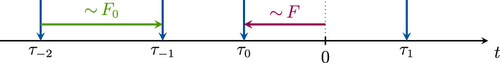
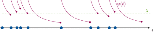
For this example, note that the hazard rate function is decreasing for any choice of the parameters. Therefore, at an arrival time , the stochastic intensity increases (the hazard rate resets to following (9)), and a subsequent arrival becomes more likely. This gives rise to bursty traffic as depicted in Figure 2.
For this process, we can also compute the distributions of the observed stochastic intensity at nonsynchronized or synchronized times:
In Figure 3, we depict the distributions , F, G, and as well as the hazard rate function for the case and (with average intensity ). In this particular case, the nonsynchronized OSI distribution is uniform in [0, 2].
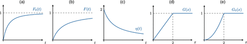
Notes. (a) Interarrival cdf. (b) Age cdf. (c) Hazard rate. (d) Stationary observed hazard rate cdf. (e) Observed hazard rate upon arrival cdf.
3. Local Memory Systems and Optimal Storage Policy
We start by rigorously defining our model for a local memory system. Requests from a catalog of N equally sized items are received (we defer the discussion of heterogeneous sizes to Section 7). We model item requests by stationary stochastic point processes , , which are defined on a common probability space and with finite intensity , a measure of the popularity of item i. By appropriate labeling, we can choose (i.e., the objects are ordered by decreasing popularities). Thus, the complete request process is the superposition , and its total intensity is .
The local memory is limited, and thus, it can only keep readily available a subset of size of the items. These items can upon request be served from the local memory with lower cost than retrieving them from a central repository. This formulation is quite general, and it subsumes the typical notion of caching, which is useful in many applications.2 Mathematically, the local memory can keep at any point in time a subset
We call the process the storage process of the system, where denotes the subsets of with size less than C.
For a given storage process, we can define the hit-counting process of the local memory system as
(i.e., the thinned process that counts the requests of objects only if they are stored in memory at the request time). The mean intensity of the process is called the hit rate, and accordingly, it satisfies .
The natural objective in this setting is to maximize (i.e., the rate at which requests can be served directly from the local memory) by choosing an appropriate policy that defines the storage process . However, this policy should be causal (i.e., it cannot make use of future information). Otherwise, the policy that only stores the next arriving item achieves a maximum rate using only one unit of memory for any N, and the problem is trivial. This is where the predictability notion introduced in Section 2.1 becomes important.
Let us denote by the natural history of the ith request process , and is its stochastic intensity with respect to . Define as the aggregated history (i.e., the information about all arrivals up to time t). Note that we are not assuming independence between the request processes. We have the following definition.
Consider a local memory system with request processes , aggregated natural history , and capacity C. A causal memory management policy is a stationary -predictable stochastic process , with values in the space of all subsets of of size at most C (equipped with the discrete -algebra).
We would like to characterize the causal policy that maximizes the hit rate . We need the following assumption.
The aggregated process is simple, and each process admits a stochastic intensity with respect to the aggregated natural history for all .
Note that the stochastic intensity need not be equal to the individual stochastic intensity because of crossinformation across arrivals. However, the average intensity should still satisfy . The following example illustrates this fact.
Consider the following process; objects are requested alternatively one after another. When a request for item i arrives, an exponential distribution with parameter is started, and after expiration, the request for object arrives (with the cyclic convention ). Let denote the requests for item i and denote the total request process. Then, it is clear that is a renewal process with interval length following a hypoexponential (phase-type) distribution (i.e., the sum of independent exponentials with parameters ). In this case, by Equation (9), , where is the hazard rate function of the resulting hypoexponential, and it is the same for all i.
However, when looking at the aggregated history, it is clear that arrivals for item i can only come at rate after a request from process ; therefore,
Assumption 1 is also needed to guarantee the existence of ; as an extreme example, consider in particular two processes and (i.e., a delayed version of the first with fixed). Then, their stochastic intensities with respect to their own natural histories are just delayed versions of one another: . However, in the combined history of both processes, the stochastic intensity of process 2 is zero everywhere except that it degenerates into Dirac functions at the -shifted points of process 1. Hence, these processes do not have a stochastic intensity in the sense of Definition 2 (which requires a proper stochastic function ) with respect to the combined history of both processes. Assumption 1 ensures that these pathological examples with complete correlation are excluded.
We are now in position to compute the stochastic intensity of the hit process.
Let be a causal policy. The stochastic intensity of its associated hit process defined by (16) with respect to the aggregated history is
We apply the smoothing Equation (4) in Section 2.1. For an -predictable process , we write
The second equality follows from the smoothing Equation (4) because by Assumption 1, the stochastic intensity of with respect is . The last equality is because of the process being predictable. This is the case because is causal and thus, measurable; therefore, is also measurable for all i.
Because the identity holds for any -predictable process , the converse implication in the smoothing formula establishes (17). □
Define now the policy as follows. At any point in time, rank the items by decreasing stochastic intensities , and store the C highest; ties may be broken arbitrarily. Note that this policy maximizes the sum of the stochastic intensities of the items in memory
(
Note from Equation (17) and the construction of that for any realization,
The first inequality follows by taking expectations on both sides with respect to the joint probability measure of the arrival processes (nonsynchronized with arrivals).
To derive the second statement, we begin by observing that by definition (Equation (16)), for any , so must also be simple. Therefore, it suffices to show that for any causal policy, (i.e., the hit rate is the total rate “thinned” by the hit probability). This is a natural property but nontrivial because the thinning is not independent of the arrival process.
From the superposition properties of stationary point processes (Brémaud 2020, example 7.2.11), under Assumption 1, the aggregated process is simple, and for any event A, we must have
To interpret the above, note that given a point in occurring at time 0, is the probability that this point comes from process i. Now, apply (20) to the event :
We now compute as
Now, return to (17) and its expectation at :
Because is Ft predictable for any causal policy, it follows from Papangelou’s formula (Equation (5)) that
Summation over i gives together with (21), as claimed, and the result follows. □
Thus, Theorem 3 gives a clean formulation of what the optimal policy is: just keep track of the most likely arrivals in the system given the complete past history of the arrival stream. In particular, this generalizes Panigrahy et al. (2022) to general (possibly correlated) superpositions that provided that they satisfy Assumption 1.
3.1. The Case of Independent Request Streams
In the preceding analysis, computing the optimal policy requires knowledge of the stochastic intensities with respect to the aggregated history. This may require the knowledge of the underlying correlations. This is greatly simplified if the request processes are independent.
Consider now a local memory system with capacity C fed by N-independent stationary request processes with average intensities as before (in decreasing order). Again, let be the natural history of the ith process, and let be the aggregated history. Again, let denote the Palm probability of the superposition process, and let be the Palm probability of the ith process.
The superposition of independent simple processes is simple (Baccelli and Brémaud 2013, property 1.1.1), and besides Equation (20), we also have (Brémaud 2020, example 7.2.8)
The interpretation of Equation (22) is the following; in order to compute Palm probabilities given that the point comes from process i, we must use the Palm probability for process i and the stationary probability for any other , and the processes remain independent.
This, in turn, allows us to prove the following property.
If is the superposition process, then is a history of . Moreover, is a stochastic intensity for process i with respect to the enlarged history , and the total stochastic intensity of is simply .
First, is measurable for all because the sum function is measurable and . Second, is the stochastic intensity of with respect to the shared history because the conditional expectation given coincides with the conditional expectation given for any random variable independent of with . This fact is, in turn, a consequence of the independence of the filtrations and that is generated by events of the form with , . Finally, that is the stochastic intensity of with respect to follows immediately by linearity of conditional expectation. □
The above lemma guarantees that the stochastic intensity of process i is not altered by superposition with other independent processes; there is no crossinformation between the processes. In particular, Assumption 1 is satisfied, and therefore, we can replace by in Theorem 3 to obtain Theorem 4.
(
At any point in time, rank the items in decreasing order of their individual stochastic intensities .
Store in memory the first C objects in the ranking.
Any other causal policy will satisfy and .
The above theorem characterizes the structure of the optimal causal policy for any superposition of independent request processes (i.e., where no additional information is available about the future other than the natural history of the requests and where there is no crossinformation between them). If the processes are correlated among them, this statement will not be true in general, and we will have to keep track of the shared stochastic intensity with respect to the common history .
We now analyze some examples where the above policy can be further characterized. The simplest is the Poisson case.
(
(
Rank all contents in decreasing order of the current interval hazard rates, .
Store in memory the first C objects in the ranking.
As we can see, the role of the hazard rates is crucial as already identified in Ferragut et al. (2016) for timer-based caching. Different monotonicity assumptions on these hazard rates lead to completely different optimal policies as we shall see in Section 6.
An issue with the optimal policy is that its main performance metric, the hit rate, cannot be computed exactly except in some special cases. We now derive an asymptotic result that characterizes the optimal policy for large-scale systems and allows us to calculate asymptotic performance limits.
4. Large-Scale Analysis of the Optimal Causal Policy
In this section, we will present results concerning the asymptotic behavior of the optimal policy in a large-scale regime, where both the system load and the memory size scale appropriately to infinity. For this purpose, we need to introduce more structure into the problem; in particular, we will assume that requests for different items come from independent processes from a common scale family in the following sense.
Consider a base process with unit intensity , natural history , and stochastic intensity with respect to . In particular, . For our asymptotic analysis, we specify our scale family as satisfying the following.
The request processes for items are independent with stochastic intensities
A construction that generates processes satisfying this assumption is to take independent copies of and set (i.e., rescale the time axis).
It is direct from Definition 6 and Assumption 2 that if is the observed stochastic intensity for process i, then the following scaling relationships hold:
(
We can also express the age distribution and hazard rate function for the ith request process in terms of the base case , :
4.1. Threshold Characterization of the Optimal Policy
Under Assumption 2, the optimal policy of Theorem 4 can be recast as follows; at any given time, we have a sample of random variables , each representing the observed stochastic intensity (for the renewal case, hazard rate since the last request) of the ith request process. Because the processes are independent, the ’s are independent but nonidentically distributed; in fact, .
According to Theorem 4, an item will be stored in memory if and only if its OSI is one of the C highest. An alternative way to cast this optimal policy is to consider the empirical distribution of the observed stochastic intensities defined by
Introducing the quantile function (inverse of the empirical distribution)
The random variable acts as a threshold in the OSI that determines the items to optimally store in local memory. Equivalently, , where are the order statistics of the sample .
We will pursue asymptotic results for a system with a very large catalog size N. If we can find a suitable limit for the empirical distribution as and if the memory size scales linearly with N such that , then the quantile should approach a limit (i.e., the large-scale behavior should resemble a policy with a fixed threshold in OSI).
Because the ’s are not identically distributed, we cannot use classical Glivenko–Cantelli arguments for empirical distribution convergence. Nevertheless, we will show that a suitable limit arises under Assumption 2 if the system load as defined by the request intensities also scales appropriately with N.
4.2. Scaling of the Request Intensities
We will construct a sequence of systems indexed by N, the number of arrival streams or in other words, items in its catalog. Denote by the arrival rates of the system of size N, with the above convention that . We may think of these points as a discrete measure on the axis of possible process intensities. Normalizing this measure to total unit mass, we may write its distribution function
The total arrival rate for system of size N can then be expressed as
Our limit theorems will assume that this family of discrete distributions has a limit with .
There exists a fixed distribution L with no atoms at such that when . Here, denotes usual weak convergence of probability distributions.
To gain some intuition on the above condition, we turn to the following important example.
(
In order to model this in our setting, we can use the following arrival rates for the Nth system:
Because the above convergence is point wise and the limit is continuous, we have given by
In the limit, the popularities follow a continuous distribution over : namely, a standard Pareto distribution with tail parameter .
If (i.e., the popularities are light tailed), some objects are extremely more popular than others; in this case, L does not have a finite mean. If instead, , where popularities are heavy tailed and thus, more homogeneous, L has finite mean . For , the system degenerates into every object having the same popularity, and thus, L is the step function at .
It is also worth observing that the total arrival rate of the Nth system satisfies
In particular, with our scaling, the total arrival rate as , albeit at different rates depending on the tail parameter .
4.3. Asymptotic Behavior of the Optimal Causal Policy
We now return to our family of systems indexed by N with independent request streams coming from a common scale family with base distribution (Assumption 2) and incorporate the scaling in Assumption 3 on the arrival rates . Namely, their empirical distribution in (27) has a weak limit .
If we look at each system at a fixed time , we obtain a sample of the current observed stochastic intensities . Considered collectively that for all , these random variables constitute a triangular array; without loss of generality, we may assume that they are all defined in a common probability space .
For each N, we can define the random function by Equation (24). The main result below concerns the asymptotic behavior of these empirical stochastic intensity distributions.
Consider a family of local memory systems indexed by N with request processes satisfying Assumption 2 and with intensities satisfying Assumption 3. Then,
Moreover, assume that the memory size of the Nth system satisfies with .
Then, if is a continuity point of the quantile function , the random threshold defined by Equation (26) converges P almost surely to .
The proof begins by computing the expected value of the random function :
We first show that as distribution functions, as . To do so, it is convenient to interpret (30) as follows; consider a pair of independent random variables in with respective distribution functions and . Then, is the distribution of the product . Indeed,
Now, consider the limit in the distribution of the pair . Because of their independence and because , the limit corresponds to the distribution of , a vector of independent random variables with marginal distributions and . By continuity of the map , we conclude that . It remains to compute the distribution function of the latter product:
We conclude that as . Equivalently, we have point-wise convergence at any continuity point of .
To relate the mean function to the stochastic one , we now resort to Shorack (1979, theorem 2.1), a generalization of the classical Glivenko–Cantelli theorem for empirical distributions for random variables that are not identically distributed. The theorem states that in the probability space where the triangular array is defined, we have
In particular, with probability 1, as for all . Combining this with the previously obtained point-wise convergence of , we conclude that almost surely at any continuity point of , and thus, .
Finally, convergence of now follows from the fact that convergence in distribution implies convergence of quantiles; specifically (van der Vaart 1998, lemma 21.2), is equivalent to for all continuity points of . See also Proposition A.2 in Appendix A.1. □
We have thus established that the optimal causal local memory policy converges in the large-scale limit to a deterministic threshold policy in the observed stochastic intensities. Specifically, when memory scales as a fraction c of the catalog, a large-scale system should store at any given time the items whose current OSI exceeds a threshold chosen as the quantile of the limit distribution in (29).
5. Asymptotic Optimal Performance
In this section, we analyze the performance achieved by the optimal policy in the large-scale limit. As discussed in Section 3, performance in local memory systems is measured by the hit probability or equivalently, the hit rate .
We will find it more convenient to derive expressions for the complementary miss probability and the miss rate . Referring back to Equation (21), we can write the following expressions for these quantities in a system of size N.3
The key challenge in the evaluation of the above formulas is to compute (i.e., the probability that an incoming arrival does not find its file in local memory). In the optimal policy for fixed N, the determining condition is whether the observed stochastic intensity of the requested item finds itself among the C largest. To correctly evaluate this probability, however, we must recognize an asymmetry. The competing are being evaluated at a time not synchronized with their arrivals and thus, follow independent distributions ; for the item in question, we must use the distribution that applies to synchronized sampling of the stochastic intensity.
For this reason, to analyze the comparison, it is convenient to define the empirical distribution
The above equivalence assumes that there are no ties in the comparison of the OSIs; to simplify the analysis to follow, we will make this a standing assumption in this section.
For each and , .
Returning to (32b), we may now express the performance criterion of the optimal policy as
We now outline informally the essence of the analysis that follows. Because the empirical distribution corresponds to intensities, which are sampled at a nonsynchronized point, its asymptotic behavior under the assumed scaling should follow the conclusions of Theorem 5 (i.e., converge to the distribution ). Under , we have , so we should have as .
This leads us to consider the approximate formula
Invoking the distribution of intensities in (27), we may express the approximation as
Under Assumption 3, . The integrand function is bounded by , invoking (7); if it is continuous, the right-hand side will converge to the corresponding integral with the limit distribution . This formula for the asymptotic optimal miss rate is the main conjecture that we will prove in Theorem 6 below, making rigorous the preceding approximate reasoning.
We will require some additional technical conditions.
For continuity of , it will suffice to guarantee it at the atoms of the measure (i.e., the discontinuities of ); denote this set by , and recall by Assumption 3 that . Analogously, denote by the set of discontinuities of , and denote by ; we will require for our limit theorem that .
To carry out the limit result for in (34), we will treat separately two cases in regard to the uniform integrability of the family of popularity distributions . The family is uniformly integrable if
Uniform integrability is a standard assumption (see, e.g., Billingsley 1999, section 1.3) that connects convergence in distribution with convergence of the first moment. In particular, if and the ’s are uniformly integrable, then
A partial converse also holds; if , with first moments satisfying (36), the family must be uniformly integrable.
The Zipf family considered in Example 6 has continuous limit L and thus, satisfies all necessary continuity assumptions. Furthermore, the family is uniformly integrable for ; for , the limit distribution has infinite mean.
We are now ready to state our main performance result.
(
The proof is given in Appendix A.
The result states that for a uniformly integrable scaling of popularity distributions, under some regularity assumptions, the miss rate of the optimal policy scales linearly with N with a proportionality constant given by the integral in (37), where the distribution function of the OSI under synchronous sampling appears explicitly. On the other hand, the nonsynchronous distribution G of the OSI also influences the formula because it determines the distribution in (29), whose quantile is the asymptotic threshold .
(
Note that
Note regarding Equation (38) that the numerator is bounded by ; indeed, we have from Lemma 1, and L has unit mass. As the first moment of this distribution (in the denominator) becomes larger, the miss probability is smaller. This suggests that for L with infinite first moment, the miss probability will be zero. This is indeed true, but we must provide a separate argument because uniform integrability will not hold in this case. Our strategy will be to show that a suboptimal policy (the static one with ) already achieves vanishing asymptotic miss probability.
(
The first inequality is immediate by optimality of . So, we focus on the static policy, where misses are certain for ; therefore,
Because and , we have that . Then,
For the denominator, we have (Billingsley 1999, theorem 3.4)
As a comment on the above results, we note the following. When the distribution of item intensities is not uniformly integrable as, for example, in the Zipf case with , items with the largest intensities dominate the rest; thus, it is natural that the static policy would achieve asymptotic optimality and perfect performance regardless of the interarrival distribution. Note, however, that such convergence may be slow; we refer to Section 8 for examples.
In the more interesting case of uniform integrability with less disparate popularities, any causal memory management policy will incur some performance penalty; the minimum miss probability achieved by the optimal policy can be computed explicitly from the interarrival distribution characteristics and the storage fraction c.
6. Threshold Policies and Their Timer-Based Counterparts
In Section 4, we found that the optimal causal policy could be expressed in terms of a threshold on the observed stochastic intensity. This threshold is stochastically varying but converges in our large-scale regime to a deterministic constant.
This motivates us to look at policies that are defined by a deterministic threshold (i.e., where one keeps in memory items with stochastic intensity larger than ). An immediate observation is that in such policies, the memory constraint C would not be satisfied in a strong way at all times. Rather, we must replace it with the soft constraint where the average memory occupation is C. We now make this formal.
6.1. Threshold Policies and Memory Occupation
Consider a local memory system with independent request processes , aggregated natural history , and stochastic intensities . Consider the following threshold policy:
(i.e., the store in memory of all of the items that have current stochastic intensity above the threshold ).
Because the ’s are stationary, the intensities are also stationary, and thus, we have a stationary and causal policy. The memory occupation of this policy is now the stationary random process:
Its average can be computed as (using as a sampling point)
Note that is decreasing from N to zero as goes from zero to . In order to have a fair comparison against a fixed memory constraint, define the threshold as
Thus, is the quantile of the average of the distributions of the stochastic intensities observed at time 0. From the right continuity of the distribution functions, it is easy to check that with equality if is a continuity point of the quantile function. We shall assume this henceforth to simplify exposition.
Because the arrival processes are independent, the random variables are independent, and thus, we have the following proposition.
Assume that the above quantile is exact in the sense that . Take with . Then, for any ,
The proof follows from the Hoeffding inequality applied to the independent Bernoulli random variables . In fact, for any N and ,
From Proposition 1, we conclude that under independent request processes, the memory occupation of the threshold policy will not deviate much from a fixed memory policy for large N. We will use this to our advantage in Section 8.
6.2. Asymptotic Optimality of Threshold Policies
We focus now on the situation studied in Sections 4 and 5, where by Assumption 2, the request processes come from a common scale family. Furthermore, the traffic intensities satisfy Assumption 3.
In that case, , which is the observed stochastic intensity with distribution . Therefore, is the solution to the equation
Invoking Equation (23a) for the scale family and rearranging terms, we have
We are now in position to prove the following.
Consider a family of local memory systems indexed by N with request processes satisfying Assumptions 2 and 3. Choose the memory size of the Nth system as with . If there exists a unique solution to satisfying
The essential step of the proof is to show that ; this part is identical to the proof of Theorem 5. The result then follows from the convergence of quantiles.
Let us now analyze the asymptotic performance; considering an object i, its miss probability is given by
Therefore, the total miss probability for system N is given by
We can then state a result analogous to Theorem 6 and Corollary 1 for the asymptotic performance.
Under the conditions of Theorem 6, the asymptotic miss probability satisfies
The proof is substantially easier than in the case of Theorem 6 because the threshold is deterministic instead of depending on the state of the remaining processes.
Indeed, by Lemma 1 and the fact that , we see that the function is uniformly bounded for all N. Taking proper account of continuity as in Theorem 6, the numerator converges as stated. For the denominator, we invoke uniform integrability.
The main conclusion of this analysis is that under the above assumptions, a deterministic threshold policy with a soft memory constraint is asymptotically equivalent to the optimal causal policy derived in Section 3 both in terms of memory usage and in terms of performance.
We shall show now that there is a strong connection between threshold policies and timer-based ones.
6.3. Connection with Timer-Based Policies: Monotone Hazard Rates
To end this section, we would like to highlight a strong connection between threshold policies and timer-based ones in the case where the requests follow renewal processes. Timer-based or time-to-live caching has been a long-standing idea in local memory systems; here, each time a request for item i occurs, a timer is started, and the item is kept in memory up to the timer expiration. When a new request arrives, the timer is reset. TTL policies were first analyzed in terms of point process requests in Fofack et al. (2014), and the optimal timers under stationary requests were obtained in Ferragut et al. (2016).
Consider the policy defined in (43) with deterministic threshold from Equation (46). Assume that the incoming processes are renewal and that the interarrival hazard rates are strictly monotonically decreasing over the distribution domain (as in the Pareto parametric example). Assume for simplicity that the threshold lies in the range of the function , and define
Then, because is decreasing, we have
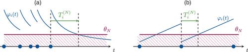
Notes. (a) Timer-based caching for decreasing hazard rates. (b) Timer-based prefetching for increasing hazard rates.
An analogous discussion is valid for monotonically increasing hazard rates; here, the likelihood of a subsequent request is smallest immediately after receiving one, and thus, caching is not useful. Instead, it was proposed in Ferragut et al. (2024) to remove the item and prefetch it at an appropriate later time. In fact, this strategy can also be cast as a threshold policy by observing (see Figure 4) that
7. Extension to Heterogeneous Object Sizes
The preceding model assumes that objects have equal sizes; they all have the same impact on memory, and the natural performance criterion is the hit probability determined by whether the object can be (fully) recovered from local memory upon request. In practice, items can have different sizes and therefore, unequal memory cost. Also, one can consider in the performance the value of a partial recovery of the object. We now formalize this approach, which was first proposed in Panigrahy et al. (2022), and we show how the previous results can be extended to incorporate this case.
Consider a local memory system fed by a family of request processes with intensities , natural histories , and stochastic intensities . Again, let be their superposition, and let be the aggregated history. Assume that each object i has a size and that the system has total memory C.
A causal policy will now be an -predictable stochastic process , where represents the fractions of each file stored in the local memory. For feasibility, the policy should satisfy the memory constraint
Thus, we are allowing fractional caching (i.e., only part of the item to be stored in memory).
Assume that whenever a request for item i arrives at time t, it can recover from the local memory and derives a utility from this amount of content , where is a concave function. In this scenario, the analogue of the hit process is the following utility process:
The process is a measure-valued process that stores the utility derived from the local memory retrievals. For the special case where , we recover the byte-counting process in Panigrahy et al. (2022) because it keeps track of the amount of data recovered from the local memory in any time interval.
Now, let this local memory system be fed by a superposition of request processes satisfying Assumption 1. We have the analogue of Lemma 2.
Let be a causal policy. The stochastic intensity of the utility process (49) with respect to the aggregated history is
The proof is similar to the proof of Lemma 2, changing the predictable process for the fractional caching version , where is predictable by assumption.
Consider now the policy defined by solving the following optimization problem:
We then have the analogue of Theorem 3.
Given a local memory system with total memory C fed by a family of stationary point processes, with aggregated natural history , satisfying Assumption 1. Assume that the item sizes are and that the system may store fractional items. Then, for any causal policy , the stationary utility rate satisfies
The proof follows along the same lines of Theorem 3 by observing that the policy satisfies Equations (51) at all times.
(
Rank the contents in decreasing order of .
Choose the first K objects satisfying
where denotes the ordering permutation of the first step.Take for and .
In other words, at all times, store the most likely upcoming requests as dictated by the stochastic intensity up to filling up your memory.
Note that the policy in Example 8 ranks the objects again in terms of the stochastic intensity independently of the object size. In particular, the optimal policy can be cast as a dynamic threshold policy, where the threshold is the stochastic intensity of the Kth object (i.e., the one that completes the memory allocation). Because of this fact, we think that the asymptotic results of Sections 5 and 6 can also be extended to this case under the appropriate scaling assumptions. This topic will be pursued in future work.
8. Parametric Examples and Simulations
In this section, we provide some interesting parametric examples to highlight the power of the results, in particular enabling us to compute sharp estimates for the performance of a local memory system. We must specify the interarrival distribution of our scale family of request processes and the distribution of popularities. We begin with the Pareto–Zipf combination, which was already introduced in examples above. We then analyze a further example with increasing hazard rates.
8.1. Pareto Interarrival Times and Zipf Popularities
Consider first the Pareto interrequest times introduced in Section 2.3 with tail parameter . As we already mentioned, this family represents bursty traffic with decreasing hazard rates. For the base (unit intensity) process, we have the following distribution for (nonsynchronized) observed stochastic intensity:
Combine it with the Zipf popularities with tail parameter introduced in Example 6 with limit distribution
By appropriately integrating Equation (29), we can obtain the asymptotic distribution:
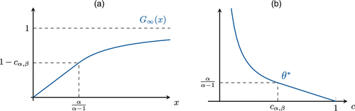
Notes. (a) Limit distribution G∞. (b) Threshold fixed point.
Because is strictly increasing, we can now solve for the unique asymptotic threshold as a function of the memory size c. Imposing , we get the following result:
In the case , it is easy to see that the measures are uniformly integrable, and thus, we can compute the miss rate estimate from (37):
Substituting the appropriate threshold and noting that , we reach the following result for the asymptotic miss probability:
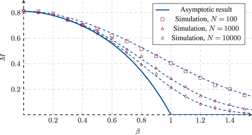
In Figure 6, we plot the asymptotic miss probability of Equation (53) for fixed and c as a function of the popularity tail parameter . We also compare it with the asymptotic miss probability of the static policy, which is derived in Ferragut et al. (2016) and is given by for . The optimal policy has the most advantage when popularities are more homogeneous; in particular, as , we have for any . The gain is larger as decreases; the optimal policy capitalizes on the burstiness of the incoming traffic captured by the hazard rates.
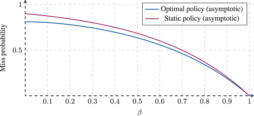
Notes. Pareto interrequest times with and . The static policy was added for comparison.
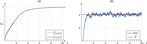
A second observation is that convergence of the empirical distribution of the OSIs is very fast. In Figure 7, we plot a simulated sample in the steady state of for items for and as an example. We see the convergence to as established in Theorem 5.
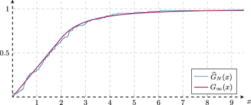
Note. Pareto requests with and Zipf popularities with .
Moreover, because convergence to is fast, convergence of the random threshold is also fast. We plot panels (a) and (b) of Figure 8 two examples with the same parameters as above for N = 1,000 and 10,000, respectively. The threshold process is approximately constant for large N around the value .
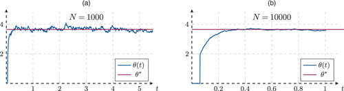
Notes. (a) Catalog size N = 1,000. (b) Catalog size N = 10,000.
This last observation is crucial for developing finite N approximations for the performance. Because of the fact that when , the family of distributions approaches nonuniform integrability, convergence of the miss rate estimate , the total rate , and the miss probability is slow around this value as depicted in the simulations shown in Figure 9.
Notes. The solid curve represents the asymptotic result (53). Dots represent simulation results for different values of N. The dotted lines represent the finite N approximation (54).
In order to compute finite N approximations, we use the intuition developed in Equation (35); that is, we compute the asymptotic threshold by solving and plug in this estimate in place of the random threshold . Then, we estimate as
This turns out to be equivalent to approximating the optimal performance for that of the fixed threshold policy discussed in Section 6, and it is numerically easy to compute, even for distributions that do not have closed-form expressions as in this case. Therefore, this procedure provides sharp estimates of the maximum achievable performance for any policy and finite N. An example of this approximation is depicted in the dashed lines in Figure 9.
8.2. Erlang Interrequest Times and Zipf Popularities
We now turn our attention to a different example, where the hazard rate of the interrequest distribution is increasing. This leads to a totally different behavior; for instance, caching is not a good idea in this setting because upon receiving a request, a subsequent request becomes less likely. It is actually preferable to remove the content from memory and prefetch it again closer to request time (Ferragut et al. 2024).
Of course, the optimal memory management policy designed in Section 5 does this automatically by keeping track of the hazard rates, and all of the asymptotic results derived for it are still valid in this case.
To illustrate this behavior, we choose the interrequest times to be distributed as an Erlang distribution with k stages and appropriate means. For , this corresponds to the Poisson process because interrequest times become exponential. As k grows, the process approaches deterministic interrequest times, and thus, the traffic pattern becomes more regular.
To be precise, let the base interrequest distribution be Erlang with k stages and mean of one (so ). This corresponds to the following:
This yields the following nice formula for the hazard rate function:
We do not have analytical expressions for the age distribution or for the observed hazard rates, so must be estimated numerically. We do so for the Zipf popularity distribution limit introduced above. We plot the resulting distribution in Figure 10 together with a simulation of the empirical version for N = 1,000, showing good convergence. Also, in Figure 10, we show the threshold evolution over time for the optimal policy, showing convergence to the numerically computed limit .
Notes. (a) Empirical distribution of the observed hazard rates for N = 1,000 and its limit G∞(x). (b) Threshold process evolution and predicted limit θ* numerically computed.
Finally, in Figure 11, we plot the asymptotic miss probability of the optimal policy numerically computed from Equation (38) as well as a simulation of the optimal policy for N = 1,000 as a function of parameter . As discussed above, convergence to the performance limit is slow when approaches one, so we compute the performance estimate from (54), which also corresponds to the optimal prefetching policy from Ferragut et al. (2024), showing good fit. As a comparison, the classical LRU policy is also simulated for the traffic pattern. As we discussed above, classical caching performs badly because of the regularity of the request process.
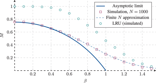
Notes. The solid curve represents the asymptotic result. Squares represent simulation results (N = 1,000), and the numerical approximation from (54) is shown by the dashed line. For comparison, LRU simulations are also shown.
8.3. Practical Implementation
Although our paper is focused on theoretical results for the optimal management of local memory systems, it is important to discuss possible practical implementations of the optimal policy. From Theorem 3, we know that the key point to implement the optimal policy is correctly estimating the stochastic intensities of the underlying request processes, a well-known hard problem in statistics (Daley and Vere-Jones 2003, chapter 7.5) with few results.
In the case where the incoming processes are independent and renewal processes, the problem boils down to estimating the hazard rate function of each stream based on previously recorded requests. Hazard rate estimation from life tables and for discrete random variables is a well-studied issue, with estimators such as the Kaplan–Meier estimator for the hazard rate and the Nelson–Aalen estimator for the cumulative hazard rate, respectively (Colosimo et al. 2002). In the continuous setting, some sort of kernel smoothing must be done (Tanner and Wong 1983) because by definition, the hazard rate depends on the underlying density of the distribution, so the problem is completely related to kernel density estimation.
Nevertheless, in our case, we can propose a practical algorithm along the lines of the Nelson–Aalen estimator. We first discuss this for a given item i, so we drop the dependence on i to ease the notation. Begin by observing that the hazard rate is given by
Keep track of the observed interrequest times up to time t.
Construct the ordered sample .
Measure the current elapsed time because the last arrival .
Find k such that
(i.e., the interval in the sample that contains the current elapsed time).
Estimate the hazard rate at elapsed time as the slope of the empirical cumulative hazard rate between times and , which can be directly computed as
Note that the computational complexity of this algorithm is high because we must keep track of a large-enough sample of interarrival times (something that is difficult to achieve for less popular items), and we must do so for each item in the catalog. We must also keep these interarrival times sorted and find the correct interval to evaluate the slope dynamically as time elapses.
This is why more computationally efficient algorithms are needed. In particular, the classical and simple LRU algorithm seems well suited but only in the case of decreasing hazard rates or bursty traffic. For more regular traffic, like in the increasing hazard rate case, the problem is still open.
9. Conclusions
This paper analyzes the optimal management of local memory systems with tools of stationary point processes. As a first contribution, we provided a rigorous setting for this problem, and under suitable assumptions, we characterized the optimal policy (in the sense of maximizing hit rates) to store in memory at every moment the items corresponding to the highest stochastic intensities.
From this starting point, for the case of independent request streams, we analyzed the limiting behavior of the optimal policy as the catalog size when a fixed fraction c of items can be stored. Assuming that item request processes come from a common scale family with intensities that have a limit in distribution, we proved that the optimal policy amounts to comparing the stochastic intensity (observed hazard rate) of the process with a fixed threshold defined by the quantile of a certain limiting distribution function. We further characterized the asymptotic performance (miss probability) of this optimal policy.
We also analyzed optimal threshold policies for the finite N case that satisfy the memory constraint in the mean. We showed that they have the same limiting behavior as the optimal policy. Moreover, we found that for renewal traffic and monotonic hazard rates in the interrequest distribution, these are equivalent to timer-based policies, where caching or prefetching times are determined by a hazard rate threshold. We also showed that some of the optimality results presented extend quite nicely to the case of heterogeneous object sizes and fractional caching.
Finally, we presented two detailed examples of our results for the standard Zipf model of item popularities and two cases for the interrequest process. For the bursty, decreasing hazard rate case of Pareto interarrival times, we obtain closed-form expressions for the optimal asymptotic threshold and the corresponding performance. We also provide sharp estimates of the optimal performance for finite N validated by detailed stochastic simulations. For the regular, increasing hazard rate case of Erlang interarrival times, closed-form expressions are not available, but we still carry out a numerical validation of the asymptotic threshold and performance. We also use this example to exhibit the significant superiority of the optimal policy in comparison with the popular LRU policy in contrast with the bursty case where LRU has good behavior.
For future research, we may explore the application of our machinery to characterize optimality for other kinds of request traffic: Markov-modulated Poisson processes to account for time variations, more general mixtures of traffic from different sources, and possibly, heterogeneity in item sizes as well as different popularity distributions.
Also, note that as presented, the optimal policy serves as a fundamental limit on the achievable performance but not necessarily a practical algorithm because it requires knowledge of the relevant item intensities and hazard rate distributions. This poses the question of possibly learning this information from the actual request data and alternatively, designing an eviction policy that does not make explicit use of these quantities but approximates optimal performance in practice; to some extent, LRU achieves this in the bursty case, but a counterpart for the increasing hazard rate is currently open.
Appendix A. Proof of Asymptotic Performance
In this section, we will provide a proof for our main result on asymptotic performance of the optimal policy for the uniformly integrable case. Referring back to Section 4, we begin by restating Equation (34):
To compute each term on the right, we must invoke the distribution of under the Palm probability; it would be more convenient if the right-hand side of the inequality does not depend on i. For this purpose, we will bound the quantiles obtained from with those of defined in (24), which include all items; as usual, is the corresponding quantile function. The key observation is that the contribution of the ith item to the empirical distribution of all OSIs is at most and therefore, negligible in the limit as N tends to infinity. More precisely, we have Lemma A.1.
Recalling the definitions (24) and (33), we can write
In the preceding identity, the right-hand side is the difference of two numbers, both in [0, 1]; therefore, . This holds for every x and for each i. □
We will now make use of this lemma to bound the distribution of as required for (A.1) with that of . However, this change brings a new difficulty because and would not be independent. For this reason, to calculate the distribution, we will use a coupling argument and consider independent versions of the corresponding random variables.
(
The proof is based on a coupling argument where we consider independent copies of the OSIs. The distributions of these copies mimic the distributions of the OSIs at an arbitrary time (that is, under the probability measure ) and upon an arrival at time (that is, under the Palm distribution ). More precisely, consider two independent, row-independent triangular arrays
Let
Analogously to Lemma A.1, we have
For each and , the random variables
To bound the probability on the right-hand side, observe that from (A.3), we have
Focusing momentarily on the upper bound, we can write
Multiplying by and averaging over I, we obtain from (A.5)
Invoking (A.4) and Expression (A.1) for the miss rate, we conclude the proof. □
A.1. Convergence of Quantiles
Our next step is to compute the limit as under suitable conditions of the lower and upper bounds in (A.2). We will use the convergence of Assumption 3, but we also need to address the convergence of and the distribution of quantiles for the random function .
Recall that by Theorem 5, we have with probability 1, where is defined by (29). A standard result that we have already invoked (e.g., van der Vaart 1998, lemma 21.2) is that convergence in distribution implies the convergence of quantiles at a fixed point p provided that the limit quantile function is continuous at p. We will need a slight generalization of this property for the case where quantiles of the sequence are evaluated at a variable point convergent to p. This is stated and proven next.
(
In the proof, we use the characterization of weak convergence in terms of the Lévy distance
Let . By continuity of Q at p, there exists such that implies . Let . Choose such that and for all .
We claim that
Indeed, for the left inequality of (A.7), let be such that . Then,
For the right inequality of (A.7), let be such that . Then,
Let . Then,
Thus, for all . □
A.2. Proof of Theorem 6
We are now in a position to complete the proof of our main result on performance.
We first establish that almost surely in . This follows by invoking Proposition A.2 at each in the set where , which has unit probability by Theorem 5; note that , which by hypothesis, is a point of continuity of .
Almost sure convergence implies convergence in probability and in distribution. Therefore, the distributions of the random variables both satisfy , a unit mass at the limit threshold. As a consequence, under Assumption 3, we have convergence of the product measures . We will use this fact to show that both bounds in (A.2) converge to the same limit, and it coincides with the right-hand side of (37).
Define for this purpose the function by . Our next claim is that
This claim is established in the mapping theorem (Billingsley 1999, theorem 2.7) provided that h is measurable and that its set of discontinuities has zero measure in the limit (i.e., ).
Because the limit measure in is a point mass, we have
Also, note that being a distribution function, its set of discontinuities is countable. Therefore, the measure on the right of (A.9) can only be positive if there exists (an atom of the measure L) such that . This would imply that and is ruled out by hypothesis. Therefore, the claim holds.
To finish the theorem, we must go from the convergence in distribution given in (A.8) to a first-moment condition. Here is where uniform integrability will come into play. It is easiest to express this via independent random variables and with respective distributions and with and , the latter with distribution L. Condition (A.8) is equivalent to the statement
Because , we have ; now, is uniformly integrable by hypothesis, so the same happens with . Now, invoke Billingsley (1999, theorem 3.5) to obtain
Thus, both upper and lower bounds in (A.2) converge to the given limit, which concludes the proof.
1 Note that is a proper random variable because and thus, is measurable for all . Similarly, any point is a random variable.
2 We specifically avoid using the term cache for our system because in caching, normally only the recently requested objects are stored, and our model aims to generalize these policies.
3 We now make explicit the dependence on the system size N because we will study the limits as .
4 If is not in the range of valid hazard rates, the equivalence also holds by allowing zero (or infinite) timers (i.e., items that are never (or always) stored).
References
- (2013) Elements of Queueing Theory (Springer-Verlag, Berlin).Google Scholar
- (2005) Measuring consistency in TTL-based caches. Performance Evaluation 62(1):439–455.Google Scholar
- (2010) The limiting move-to-front search-cost in law of large numbers asymptotic regimes. Ann. Appl. Probab. 20(2):722–752.Google Scholar
- (2014) Exact analysis of TTL cache networks. Performance Evaluation 79:2–23.Google Scholar
- (2015) Maximizing cache hit ratios by variance reduction. ACM SIGMETRICS Performance Evaluation Rev. 43(2):57–59.Google Scholar
- (2013) Check before storing: What is the performance price of content integrity verification in LRU caching? ACM SIGCOMM Comput. Comm. Rev. 43(3):59–67.Google Scholar
- (2017) A cache management scheme for efficient content eviction and replication in cache networks. IEEE Access 5:1692–1701.Google Scholar
- (1999) Convergence of Probability Measures, Wiley Series in Probability and Statistics, 2nd ed. (Wiley, Chichester, UK).Google Scholar
- (2010) Distributed caching algorithms for content distribution networks. 2010 Proc. IEEE INFOCOM (IEEE, Piscataway, NJ), 1–9.Google Scholar
- (2020) Point Process Calculus in Time and Space (Springer, New York).Google Scholar
- (2002) Hierarchical web caching systems: Modeling, design and experimental results. IEEE J. Selected Areas Comm. 20(7):1305–1314.Google Scholar
- (2002) Empirical comparisons between Kaplan–Meier and Nelson–Aalen survival function estimators. J. Statist. Comput. Simulation 72(4):299–308.Google Scholar
- (2003) An Introduction to the Theory of Point Processes: Volume I: Elementary Theory and Methods (Springer, New York).Google Scholar
- (1990) An approximate analysis of the LRU and FIFO buffer replacement schemes. Proc. ACM/SIGMETRICS 1990 (ACM, New York), 143–152.Google Scholar
- (2019) A utility optimization approach to network cache design. IEEE/ACM Trans. Networking 27(3):1013–1027.Google Scholar
- (2024) Caching or pre-fetching? The role of hazard rates. 2024 60th Annual Allerton Conf. Comm. Control Comput. (IEEE, Piscataway, NJ), 1–8.Google Scholar
- (2016) Optimizing TTL caches under heavy tailed demands. Proc. ACM/SIGMETRICS 2016 (ACM, New York), 101–112.Google Scholar
- (2018) Optimal timer-based caching policies for general arrival processes. Queueing Systems 88(3–4):207–241.Google Scholar
- (1996) Limits and rates of convergence for the distribution of search cost under the move-to-front rule. Theoret. Comput. Sci. 164(1):185–206.Google Scholar
- (2012) Analysis of TTL-based cache networks. Proc. Internat. Conf. Performance Evaluation Methodologies Tools (VALUETOOLS) (IEEE, Piscataway, NJ), 1–10.Google Scholar
- (2014) Performance evaluation of hierarchical TTL-based cache networks. Comput. Networks 65:212–231.Google Scholar
- (2012) A versatile and accurate approximation for LRU cache performance. Proc. 24th Internat. Teletraffic Congress (IEEE, Piscataway, NJ), 57–64.Google Scholar
- (2016) A unified approach to the performance analysis of caching systems. ACM Trans. Model. Performance Evaluation Comput. Systems 1(3):1–28.Google Scholar
- (2015) Transient and steady-state regime of a family of list-based cache replacement algorithms. Proc. ACM/SIGMETRICS 2015 (ACM, New York), 123–136.Google Scholar
- (1973) A unified approach to the evaluation of a class of replacement algorithms. IEEE Trans. Comput. C-22(6):611–618.Google Scholar
- (2016) Adaptive caching networks with optimality guarantees. ACM SIGMETRICS Performance Evaluation Rev. 44(1):113–124.Google Scholar
- (2010) Distributed caching over heterogeneous mobile networks. Proc. ACM SIGMETRICS Internat. Conf. Measurement Model. Comput. Systems (ACM, New York), 311–322.Google Scholar
- (1999) Asymptotic approximation of the move-to-front search cost distribution and least-recently used caching fault probabilities. Ann. Appl. Probab. 9(2):430–464.Google Scholar
- (2003) Asymptotic insensitivity of least-recently-used caching to statistical dependency. Proc. IEEE/INFOCOM 2003 (IEEE, Piscataway, NJ), 438–447.Google Scholar
- (2004) Least-recently-used caching with dependent requests. Theoret. Comput. Sci. 326(1):293–327.Google Scholar
- (2008) The persistent-access-caching algorithm. Random Structures Algorithms 33(2):219–251.Google Scholar
- (2006) Critical sizing of LRU caches with dependent requests. J. Appl. Probab. 43(4):1013–1027.Google Scholar
- (2003) Modeling TTL-based internet caches. Proc. IEEE/INFOCOM 2003 (IEEE, Piscataway, NJ), 417–426.Google Scholar
- (1971) Analysis of paging algorithms. Proc. IFIP Congress 1971 (North-Holland Publishing Company, Amsterdam), 485–490.Google Scholar
- (2014) A unified approach to the performance analysis of caching systems. Proc. IEEE/INFOCOM 2014 (IEEE, Piscataway, NJ), 2040–2048.Google Scholar
- (2017) Hit rate vs. hit probability based cache utility maximization. ACM SIGMETRICS Performance Evaluation Rev. 45(2):21–23.Google Scholar
- (2020) Network cache design under stationary requests: Exact analysis and Poisson approximation. Comput. Networks 180:107379.Google Scholar
- (2022) A new upper bound on cache hit probability for non-anticipative caching policies. ACM Trans. Model. Performance Evaluation Comput. Systems 7(2–4):5.Google Scholar
- (2010) Approximate models for general cache networks. Proc. IEEE/INFOCOM 2010 (IEEE, Piscataway, NJ), 1–9.Google Scholar
- (1979) The weighted empirical process of row independent random variables with arbitrary distribution functions. Statistica Neerlandica 33(4):169–189.Google Scholar
- (1983) The estimation of the hazard function from randomly censored data by the kernel method. Ann. Statist. 11(3):989–993.Google Scholar
- (1998) Asymptotic Statistics, Cambridge Series in Statistical and Probabilistic Mathematics, vol. 3 (Cambridge University Press, Cambridge, UK).Google Scholar