The Production of Service: A Workload View of Complementarity and Substitution
Abstract
We study optimal coordination in quality-driven rework systems, where each station contributes to an item’s quality and the likelihood of rework depends on these contributions through a production function. Our model links quality targets to processing times via Brownian hitting times and aggregates quality into rework probability. By setting quality targets, a planner jointly shapes processing times and rework rates, determining overall workload. We characterize the attainable workload region and use it to minimize effort costs in two-station networks. The optimal policy depends on (i) complementarity versus substitutability of quality contributions, (ii) each station’s quality impact, and (iii) relative operational costs. We identify three operating regimes: two corner regimes (one active station) and a network regime (both active). As complementarity increases, effort shifts toward the more cost-effective station, whereas finite capacity modifies this threshold, pushing effort toward the less constrained station. The analysis highlights how complementarity shapes efficiency trade-offs and capacity requirements. To illustrate the model’s practical relevance, we calibrate it using published operational statistics from industrial maintenance settings, in which equipment undergoes repair followed by preventive service while offline. The results show that the optimal design is robust to parameter misspecification, achieves substantial cost savings relative to benchmark policies, and can be estimated from standard operational data.
Funding: Partial financial support was provided by the Israel Science Foundation [Grant 277/21] and the Bernard M. Gordon Center for Systems Engineering at the Technion.
Supplemental Material: The online appendix is available at https://doi.org/10.1287/stsy.2025.0111.
1. Introduction
Workflows are a result of a design process. The design determines the activities or tasks to be performed and the effort exerted in each one. Once the workflow is set, one can turn to questions that are central to queueing theory, such as the optimization of waiting time. This paper concerns the design stage.
Our premise is that processing time and/or effort affects the quality of the outcome. Longer processing times improve output quality but require more capacity; at the same time, they reduce rework, making the net effect on workload ambiguous.
Rework imposes substantial financial and operational burdens across sectors. In manufacturing and other production systems, analyses of the “cost of quality” indicate that 5%–15% of sales are absorbed by quality-related costs, with internal failure costs—including rework—representing a major share (Schiffauerova and Thomson 2006). In asset-intensive industries, such as construction and maintenance, direct rework costs typically account for 4%–6% of total project expenditures, and they can reach 12%–15% in complex or poorly coordinated projects, contributing to delays and cost overruns (Love and Li 2000, Hwang et al. 2009). In healthcare, similar challenges arise; in the United States, hospital readmissions number about 3.8 million annually (13% of adult discharges) (Jiang and Hensche 2023), with an average cost of $16,037 per readmission (Kum Ghabowen et al. 2024). Preventable readmissions alone cost the U.S. healthcare system tens of billions of dollars each year—about $17 billion in Medicare acute-care payments (Jencks et al. 2009). These figures show that rework is widespread and costly, highlighting the importance of understanding how design choices and effort allocation affect performance.
The output quality of a service or production process depends on an aggregation of efforts throughout the process. The optimal coordination of efforts—for example, the one that minimizes effort or capacity costs—depends on the efficiency of the different steps (the capacity needed per improvement in the step’s output quality) and their effectiveness (the impact of quality improvement in an individual step on the overall process output).
The ideas that we introduce in this paper and the questions that we address are relevant to various processing networks where there is a clear notion of repair and maintenance activities. In such systems, the planner must decide how much effort to allocate to each activity (e.g., preventative maintenance). In production systems, software development, and project management, a processing step is often followed by a quality assurance step. The more effort allocated to the processing step, the better the quality of the product is at transfer. The operator must distribute the efforts among the stations by considering the properties (cost, capacity, etc.) of the different steps in the process.
To study these questions, we develop a model that stipulates
a relationship between a targeted quality of output and the processing time and
a mapping from the quality of output—a vector that includes quality measures for each step of the process—and the likelihood of rework: hence, the total arrival rate.
We use a threshold model. An item is released (or transferred to the next step in the process) when its state reaches a threshold. We capture an item’s state via a quality “score” that serves as an aggregation of different quality measurements. The individual score evolution in each step is described as a stochastic process. The properties that we focus on are hitting time statistics—averages and probabilities—that determine processing times in each station. The threshold—the score at which the item is released or transferred—is the design decision. Once set, it determines the processing-time distribution. This distribution—or multiple distributions when two stations operate—affects the arrival rate.
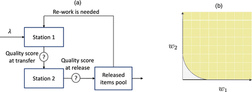
In our model, illustrated in panel (a) of Figure 1, the planner chooses the workload (effort) levels at two processing stations. The arrival rate depends endogenously on the stations’ effort levels through the rework mechanism: that is, . The presence of rework makes the attainable workload region nonlinear. This nonlinearity reflects the endogenous relationship between effort and workload, and it forms the basis for the optimization problems analyzed in the paper.
Although grounded in a dynamic quality-evolution model, the rework probability takes the simple form
We model the aggregated quality as a function that combines the quality contributions of the different stations into a single measure, which in turn, determines the probability of rework.
The aggregated-quality model captures the interaction between stations through their degree of substitution or complementarity. Intuitively, when stations are substitutes, additional effort in one can compensate for less effort in the other, whereas when they are complements, the effectiveness of one station increases with the effort devoted to the other.
We formalize these interactions in Section 4 using the constant elasticity of substitution (CES) family, a well-established framework in the economics literature for modeling the interplay between production factors (Carvalho and Tahbaz-Salehi 2019). By varying the CES parameters, we can flexibly represent different degrees of substitutability or complementarity between stations and study how these relationships affect optimal system design.
To the best of our knowledge, this is the first application of a CES formulation in a service-operations setting with quality-driven rework. Existing operations studies typically assume additive or separable relationships between process stages, where improvements in one step do not directly affect the marginal effectiveness of another. In contrast, the CES structure allows us to quantitatively vary the degree of cross-station substitution and complementarity, capturing nonlinear interdependencies that prior models abstract away. This formulation bridges economic production theory and operational design, providing a unified analytical tool for studying how interdependencies across stages shape both workload and efficiency.
Unlike in economics, where the CES function represents how inputs, such as labor and capital, combine to produce output and revenue, our operational setting endogenizes these “market” effects; the quality targets chosen at each station influence both processing times and the probability of rework, jointly determining total workload and cost. The CES specification is, therefore, the right lens here; it captures the nonlinear way in which joint effort across service stages translates into effective quality while remaining analytically tractable and interpretable. In this way, output quality—and hence, the trade-off between effort and workload—is fully internalized in our model.
1.1. Maintenance Example
The concepts of substitution and complementarity arise naturally in maintenance and reliability settings. Consider two sequential activities within a maintenance process: repair followed by preventive service. Repair represents corrective actions that restore the asset to an operational state—such as replacing a failed component, realigning a gearbox, or fixing an electrical malfunction. Preventive service then takes place while the equipment remains offline, and it involves inspections, lubrication, recalibration, and other conditioning tasks that enhance long-term reliability and reduce the likelihood of future failures. If these activities are substitutes, more extensive repair can compensate for less preventive service effort, whereas thorough postrepair maintenance may delay the need for the next repair intervention. If they are complements, the effectiveness of one depends on the other; a well-executed repair increases the impact of subsequent preventive service, whereas insufficient repair limits the benefit of additional preventive effort. We return to this example throughout the paper—first, to illustrate the theoretical mechanisms and later, to demonstrate how the model can be calibrated and interpreted.
We establish the following.
Model and workload characterization. We build our model on components (A) and (B) above and show how the decisions—the targeted quality levels—can be mapped to workload decisions. We then show that the workload feasibility set is convex; its characterization highlights the effects of complementarity on its structure (Figure 3). We prove that the higher the complementarity coefficient, the smaller the set of attainable workloads is. This implies, in particular, that the larger the complementarity, the more constrained is any cost minimization problem.
The structure of optimal designs. We show that when minimizing processing costs, corner solutions (where one station has zero effort and the other bears all of the workload) are never optimal as long as there exists some complementarity. Systems with perfect substitution generally exhibit three operating regimes: two where only one station works and one where the solution is interior and both stations are used.
This structure stands in contrast to the well-studied problem of maximizing CES utilities under budget constraints (see, e.g., Mas-Colell et al. 1995, exercise 3.C.6 and Varian 2010, chapter 4). There, with perfect substitution in the utility function, one has only corner solutions. Because the rework probability is a nonlinear function of the process quality, the solution space in our model is richer.
We show that whether the optimal station efforts are increasing or decreasing in the level of substitution depends on where the cost stands relative to a “symmetry” cost threshold. This threshold does not itself depend on the level of substitution.
The capacitated explicit solution. The characterization of the optimal solution when capacity is constrained has an informative structure; the effect of complementarity on the optimal effort mix is mediated through the capacity levels. At certain capacity levels, the “shadow price” of capacity is increasing in the complementarity; for other capacity levels, it decreases. When there are multiple types of items that “compete” for the limited capacity, the optimal mixture of workload in each station changes in nonobvious ways as capacity changes.
In Online Appendix B, we present three variants of the base model that demonstrate the flexibility and robustness of our results. These include processing complementarity (Online Appendix B.2), where the effectiveness—the quality-improvement rate—of the second station depends on the final score from the first station; rework within a finite time window (Online Appendix B.3); and rework while in Station 2 (Online Appendix B.6). We further show that these variants as well as resource-sharing and throughput-maximization problems can be formulated and solved within the attainable workload framework.
This paper does not aim to be the final word or embody a comprehensive framework for arbitrary networks. Rather, it is intended to advance key notions and initial results as well as showcase their usefulness through the insights that they provide.
Organization. We start with a brief review of the relevant literature in Section 2. The single-station model described in Section 3 serves as an important building block. We introduce substitution/complementarity in the two-station model in Section 4. This section contains the key results of the paper as they pertain to the characterization of the attainable workload region. Section 5 draws on this characterization to study process optimization. Section 6 contains a concentrated discussion of the operational/managerial implications of our results. In Section 7, we provide some concluding remarks and suggest a few directions for future research. All proofs, model variants, parameter estimation procedures, and calibration details appear in the Online Appendix.
2. Literature Review
Coordinating the optimal effort of the two stations is an instance of determining the anatomy of the service: defining its parts and their interaction. The question is one of design. Rather than taking the service content at each step as fixed, we optimize it to meet network-level goals. The anatomy of a service refers to the collection of its components, the content of each, and their interaction.
Our work speaks to the operations management literature on modeling and control of service times as well as to the literature on tandem stations with rework.
2.1. Discretionary Services
Classical models in queuing theory assume that service times are fixed and independent of the system state. Empirical evidence, however, shows that flexible processing times are prevalent in service, healthcare, and transportation systems (Chen et al. 2001, Batt and Terwiesch 2012, Staats and Gino 2012, Tan and Netessine 2014). Empirical studies in healthcare settings illustrate several behavioral mechanisms consistent with these ideas. Berry Jaeker and Tucker (2017) document an “N-shaped” relationship between hospital occupancy and patient length of stay, showing that service speed initially increases with workload but eventually declines once staff reach saturation, highlighting a speed-quality trade-off. Similarly, Kc and Terwiesch (2012) find that intensive care units discharge patients earlier when occupancy is high, which increases subsequent readmissions—direct evidence of state-dependent effort and quality-driven rework. Such state-dependent service times also make workload forecasting difficult. Finally, Clark and Huckman (2012) show that hospitals benefit from complementarities across related clinical services, where cospecialization improves quality performance. Together, these studies provide empirical motivation for our modeling assumptions regarding state-dependent effort, quality-driven rework, and cross-stage complementarities.
Our work is fundamentally concerned with discretionary services, in which working procedures are not necessarily prespecified; employees or managers get to determine the service time (or effort) and quality given to each customer. Hopp et al. (2007) is an early modeling work studying a controlled queueing model that allows the operator to decide how much time to allocate to a service. Recently, Zychlinski et al. (2026) used a Brownian motion (BM) to model the evolution of a patient’s health scores and determine optimal call-in thresholds in a hybrid hospital setting. Much of the work on discretionary services concerns single-station services (Wang et al. 2021). Here, we explore the discretionary allocation of effort across process steps/stations.
Our analysis is also related to the Brownian processing-network literature, which develops workload representations and control formulations for stochastic flow systems (Harrison and Van Mieghem 1997, Harrison 2003). In those models, the workload is obtained as a linear transformation of queue lengths that satisfies flow-balance constraints and serves as a sufficient statistic for dynamic control under heavy traffic. By contrast, our attainable workload region arises from endogenous relationships between quality, effort, and rework, yielding a convex workload space. Rather than modeling state-space collapse and dynamic control, we study how these endogenous quality interactions determine the feasible workload configuration at the design stage and its associated cost trade-offs.
Our focus in this paper is on the design of the system to determine the baseline service content. Our work takes a macro view of service times. We consider the initial design of the system—the allocation of work between two stations. Our quality progression model is not, in this paper, used to develop adaptive control for individual items, but rather, it is used to design the item-specific baseline around which further dynamic fine-tuning can be done.
2.2. Queues with Rework
Kumar (1993) studies re-entrant lines in a manufacturing setting with several machines and buffers where items visit some machines more than once at different processing stages. A single class queue with a second optional service is studied by Madan (2000). Fluid models for re-entrant lines were analyzed by Dai and Weiss (1996), who derived stability conditions for different scheduling policies.
Interest in queueing systems with rework has grown in recent years, partly because of their relevance in healthcare settings, where rework naturally arises in the form of patient readmissions—patients whose condition deteriorates after discharge and must return for additional treatment. and Shi et al. (2021) study operational decision making in such systems by explicitly modeling individual patient progression. Motivated by healthcare quality-improvement interventions, Chan et al. (2025) analyze control strategies aimed at reducing return probabilities in stylized queueing systems where customers may require multiple service episodes. Hybrid healthcare systems, in which in-person visits may be followed by unsuccessful virtual care and subsequent returns, are examined in Zychlinski (2024) and Liu et al. (2023). Recently, Zychlinski (2026) studied a queueing model of a mental health system with rework, where patients first receive group therapy and if it proves ineffective, transition to individual therapy.
The mix of items in our paper is fixed and given. Our focus is on introducing a simple but principled model of effort coordination in a multistage processing network. We cede some level of granularity relative to some papers cited above in order to understand substitution/complementarity and their operational role in a processing network.
We model quality evolution as a dynamic process of improvement and random deterioration; this allows us in a tractable way to map service-content decisions to outcomes. This tractability stems from modeling the quality evolution as a Brownian motion, which is characterized by its mean improvement speed (drift) and variability (diffusion coefficient). The BM formulation provides a coherent and analytically convenient representation of gradual improvement and potential deterioration, linking processing-time decisions to rework likelihood in a unified way.
Finally, models of complementarity and substitution have appeared before in the operations management literature. Netessine and Zhang (2005) consider externalities in supply chains and show how these depend on whether retailers’ stocking decisions are complementary or substitutes. In our case, risk is endogenized via rework. Substitution/complementarity between medical procedures/resources is also common within the healthcare economic literature (for instance, Wilson et al. 2005).
3. The Single-Station Model
For clarity, we first construct the model for a single item type. Items arrive following a renewal process with arrival rate . These are so-called “index arrivals” relative to which rework is measured.
The evolution of the quality score is modeled as a BM, whose drift captures the quality-improvement rate, and its standard deviation is the extent of randomness in improvement. The model captures item dynamics through the network. Because hitting times and rework probabilities admit closed-form expressions, it maps service-content decisions to outcomes in a tractable way.
The processing time depends on the discharge threshold l, which is a design variable. The processing time is the time that it takes a positive-drift BM to hit a target l starting at a for the first visit and zero for subsequent revisits, with drift and diffusion coefficient :
Once an item’s quality score reaches level l, the item leaves the station. Given a choice of l, the expected processing time and its variance are
After an item is released, there is a baseline probability that the initial processing resolves the problem permanently, making the likelihood of rework negligible. Define
Conditional on the problem not being—terminally and deterministically—solved, rework depends on the random evolution of the quality score. The postrelease (or discharge) score follows a BM ( postrelease), which starts at l and has a nonnegative drift that is linear in l. This relation reflects the fact that the greater the time is spent on an item, the less likely this item is to require rework. The linear choice is not arbitrary; it arises as a special case of the multistation model that we introduce in Section 4.
The diffusion coefficient of this BM is . Although the improvement rate is positive, randomness allows the quality score to hit negative levels; it reaches rework level 0 at . At this point, the item returns to the station for additional processing. The rework likelihood is then the probability that the positive-drift motion starting at l hits zero in finite time:
The rework probability decreases as l increases (hence, the average service time increases), aligning with empirical evidence on the relationship between processing time and rework likelihood. Notably, this rework probability, which is derived from our modeling framework, is consistent with the relationship , which parallels the logit estimation commonly used in the empirical literature (Kc and Terwiesch 2009, Carey 2015); see more on estimation in Online Appendix C.
Once returned for rework, the item must be brought back to quality score l before being released again. The number of processing visits is then
, and is the number of returns (rework visits). The total workload given a release-score threshold l is then
This expression implicitly handles the case where the initial score a (for the first visit) exceeds the optimal target . In that case, we treat the item as requiring no processing at all.
The workload is convex in the release score l, and the minimizer is the unique strictly positive solution to the equation
The optimal workload is given by
Notice that the maximal throughput to this single station is given by
We also observe that at optimality, the likelihood of rework , where depends only on . That is, the optimal solution adjusts the choice of l so that the likelihood of return depends only on the baseline rework probability of the item.
In systems where the arrival rate is exogenous and fixed, the load—the arrival rate multiplied by the service time—is obviously monotone in the service time. In our model, however, the workload is minimized at ; it is decreasing up to that point and increasing thereafter.1 The mathematical implication is that the mapping from workloads to targets l is not invertible; given a workload level , there can be two distinct values of l that achieve it. As stated, at , there is a unique value l (namely that achieves . Nevertheless, a mapping from w to l can be defined by imposing a choice
For the two-station model, we map the space of service-time decisions to the space of workloads. The mapping is not one to one, but as here, the mapping between the two is well defined at optimality.
(
4. Beyond a Single Station: Complementarity and Substitution
We proceed to a two-station setting with Stations 1 and 2 and a single item type. In Section 5.3, we extend the model to incorporate multiple item types with different transfer thresholds. In the context of our maintenance example, this setting represents the joint modeling of repair followed by preventive service as coordinated stages of a maintenance process, where preventive activities are performed while the equipment remains offline after repair.
We extend the notation from the previous section by adding a subscript to identify the station; for example, is the BM drift of Station , and is the target score for station i. We use l and w for the vectors and , respectively. The mean processing time is in Station 1 in the first visit, in subsequent visits to this station, and in Station 2.
Once processing at both stations is completed, an item’s total quality score at discharge is ; this value is the initial condition for the subsequent evolution of quality. After release from Station 2, the postdischarge quality evolves as a BM that starts at this discharge level , with drift (defined below) and diffusion coefficient . Hence, the drift captures how the efforts at the two stations interact—through substitution or complementarity—to influence the rate of postrelease improvement or deterioration.
The resulting return probability and expected number of visits are then given by
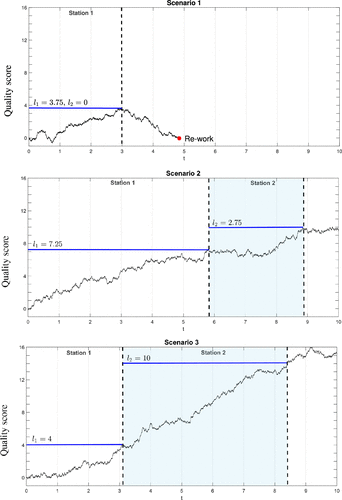
Figure 2 illustrates the evolution of the quality score during an item’s stay in the network. It visualizes the stochastic evolution of quality and the timing of rework. In all three scenarios, an item arrives at Station 1 at with score ; the quality level at each stage serves as the initial condition for the subsequent phase. In particular, the score at transfer from Station 1 to Station 2 is , and the postdischarge process starts at the discharge level , ensuring continuity of the quality trajectory across stages. In Scenario 1 (), the item is released at . Its quality deteriorates, and rework starts at . In Scenario 2 (), the item is transferred to Station 2 at and leaves Station 2 at . In Scenario 3 (), the item is transferred to Station 2 at and leaves Station 2 at . In our base model, for tractability, rework occurs only after release from Station 2; see Online Appendix B.6 for a variant where a return to Station 1 can happen while in Station 2.
4.1. Complementarity and Substitution
The efforts in both stations can be substitutive or complementary. Informally, the two stations are complements if as we increase , the incremental effect of increases. Conversely, they are substitutes if the incremental effect of is independent of , so the two efforts contribute additively to the outcome.
Because our goal is to study the design of a two-stage service process, we do not impose ex ante whether both stations must operate or only one. Instead, the optimal allocation of work across stations is determined endogenously, and the resulting design may involve effort in one or both stations depending on costs and complementarity. Complementarity and substitution, in our model, refer to how station-level efforts interact after discharge through the postrelease dynamics that govern rework and hence, the system’s effective workload.
To flexibly capture a range of such interactions, we use the CES family (Arrow et al. 1961, Sato 1967, Sato and Koizumi 1973, Stern 2011):
Observe that a single station is the same as taking . In this case, , which is consistent with our developments in Section 3 taking there.
Station Labeling. Assuming without loss of generality, Station 1 (, decision variable ) is the primary station, whereas Station 2 is the secondary station. When , the primary station is more effective, contributing more than the secondary one.
4.2. The Attainable Workload Region
In this section, we characterize the attainable workload region in the two-station setting. Beyond having its own intrinsic value, this characterization lays the foundations for solving the effort allocation problems in a structured informative way.
Given a choice , the workload in Stations 1 and 2 is given by2
We define the rate-normalized workload as
This is the workload if (hence, “rate normalized”). The actual workload is then a linear transformation of the rate-normalized workload. The vector takes values in the set
Theorem 1 is a key result. Recall that by construction, and that . Also, we let be the minimal rate-normalized workload in the single-station case with : that is,
The minimizer, , is the unique solution to
The attainable workload set is convex and can be written equivalently as
Theorem 1 establishes that the attainable workload region is convex and characterizes its boundary. Intuitively, this convexity reflects the trade-off between the workloads at the two stations; an increase in one station’s effort can partially offset a decrease in the other while maintaining the same overall system performance. The specific shape of this region depends on the parameters and , which determine the degree of substitutability or complementarity between the two stations. Proposition 1 and Figure 3 further illustrate how these parameters shape the attainable region and influence the boundary’s curvature.
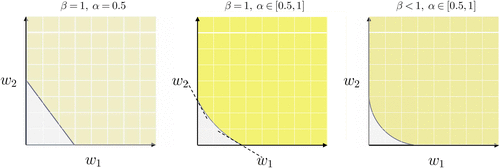
Notes. In the center panel, the boundary is convex but “hits” the axes with a strictly negative derivative (the tangents in black represent these derivatives). In the right panel, the tangents at the points where meets the axes are the axes themselves.
(
The characterization of the attainable workload region extends naturally to any number of stations n as shown in Online Appendix B.1.
A special but informative case has (stations are equally important) and (they are perfect substitutes). In this case, so that for The set in this case has the simple linear boundary shown in the left panel of Figure 3.
Next, we characterize the boundary of the set . This will be instrumental in our study of optimization problems over . In Proposition 1, is as in (7).
The derivative of satisfies the following:
Proposition 1 stipulates that for any , the boundaries of the convex set “asymptote” smoothly to the axes. This implies that for linear objective functions, there are no optimal solutions of the form or , whereas we might have some for . Indeed, from Example 1, we know that with and , the boundary is linear. Figure 3 illustrates the three possible scenarios. Importantly, when , perfect substitution in drift () could still be consistent with an optimal solution that requires the nonnegligible use of both stations. This is established in the next section.
4.3. Model Summary
Before turning to the analysis, we briefly summarize the main modeling assumptions for clarity. Items arrive at rate and evolve independently. While in Station i, an item’s quality follows a BM with drift and diffusion , and service ends when its quality score reaches a threshold . After release, quality continues to evolve with drift and diffusion , and the probability of rework is , with reworked items returning to Station 1. In the two-station setting, station-level quality contributions aggregate via the CES function . Online Appendix A summarizes all main notation and symbols used throughout the paper.
For completeness, Online Appendix C describes how the model’s parameters can be estimated from operational data; the quality‐evolution parameters are inferred from service‐time observations, and the substitution/complementarity parameters are estimated from realized rework frequencies. The Online Appendix also includes a simulation demonstrating that the proposed estimation procedure accurately recovers these parameters even in moderate sample sizes under the assumed model specification.
5. Processing Costs and Optimization
An item’s handling cost reflects the resources allocated to it. The more resources deployed, the higher the cost per unit of time. In other words, and —the cost per item per unit of time in Stations 1 and 2, respectively—would be greater for items that are more important, present a higher risk, or require more resources.
Recall that under a given decision pair l, an item (re-)visits each station times in expectation; this includes the index visit and any subsequent visits. The handling cost at each station is then given by
Recalling (5), the total journey cost for an item is, therefore,
With capacity constraints and in Stations 1 and 2, respectively, we arrive at the (constrained) optimization problem:
The solution for this capacity-constrained problem builds in a fundamental way on that of the unconstrained problem, so we start with the latter.
5.1. The Uncapacitated Problem
We consider the case where in (10). The resulting optimization problem is given by
5.1.1. Relative Marginal Cost (Relative Cost in Short).
The ratio is the marginal cost of quality improvement in Station 1; is the resource consumption cost, whereas is the time during which this effort is exerted. This is an effectiveness measure that is Station 1 focused. Similarly, is an effectiveness measure that is Station 2 focused.
The measure
The optimal solution is identical to that of the cost-normalized problem:
We write where needed to make the dependence of decisions on the relative cost explicit.
The result below—which identifies a relationship between and that depends on and —is familiar from budget-constrained production-quantity maximization with CES production functions. Although we have no explicit resource budget constraints at this point, they are implicit through the rework; our problem is, informally, a dual problem where we minimize resource consumption while satisfying a production constraint.
If there exists an interior optimal solution to (12) (i.e., with ), it must be of the form
With and —recall Example 1—the attainable workload region has a linear boundary. The slope of that linear boundary is . Hence, minimizing the linear cost function yields only corner solutions with the exception of the case where (where there are infinitely many solutions).
Under the optimal solution , the likelihood of rework depends only on and not on the relative costs. As in Lemma 1, , where is as in (6). The optimization problem adjusts the decision to the cost and substitution parameters so that the likelihood of rework is the same across all types (i.e., all combinations of cost and substitution) that have the same base rework parameter . This invariance follows from the exponential form of the return probability and the resulting first-order condition, which pin down the optimal value of as a function of alone.
Problem (12) is a minimization of a linear function over a convex region. At the optimal solution (if attained at a smooth boundary), it must be the case that the cost function is a tangent to the boundary. In Proposition 1, we saw that with , the axes are the tangents to the function at the points where it meets the axes. This means that—with the exception of the trivial case that (or )—there will be only interior optimal solutions where both ; see Figure 4. With , the tangents at both meeting points with the axes (recall Figure 3) are nontrivial. Thus, there is a value of , for which the cost function is a tangent to at and another cost where the cost function is tangential to at .
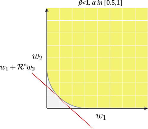
Lemma 2 characterizes the interior solution corresponding to the middle regime, where both stations are active. Theorem 2 extends that result by showing that for , the interior solution applies only within the middle regime where both stations are active, whereas the first and last regimes correspond to corner solutions where one station is inactive. In those cases, the optimal solution shifts to a corner regime, in which only one station operates because the interior condition of Lemma 2—requiring both —cannot be satisfied when the cost function is tangent to the boundary along an axis (see the center panel of Figure 3, where the tangents at the axes illustrate these corner solutions).
(
This theorem identifies the existence of three operating regimes. As long as there is some complementarity (), it is optimal to have some effort in each of the two process steps. When the postrelease drift is linear in the efforts (there is perfect substitution in the drift ()) there are three distinct operating regimes: one where no processing is optimally happening in Station 1, one where no processing is happening in Station 2, and one where some processing is required in both Stations 1 and 2. Thus, with , the exact operating regime is determined by the relative cost.
Table 1 summarizes the three operating regimes characterized by Theorem 2, indicating which stations are active and how the optimal thresholds behave across substitution levels and relative costs.
|

Table 1. Operating Regimes Characterized by Theorem 2
| Regime | Complementarity level () | Relative cost range () | Threshold behavior with |
|---|---|---|---|
| I. Station 1 only | (constant) | ||
| II. Station 2 only | (constant) | ||
| III. Both active | or ( and ) | — | decreases, and increases; as complementarity increases (), effort allocation across stations becomes more balanced |
Figure 5 is a numerical illustration of the optimal decisions in Theorem 2. It shows symmetry around a threshold value, which is explicitly characterized in part (i) of Proposition 2. For completeness, we note that the qualitative behavior of the solution extends to , where increasing complementarity (smaller ) accentuates the curvature of the response and shifts effort toward the more effective station. The limiting case corresponds to perfect complementarity, in which both stations must contribute equally.
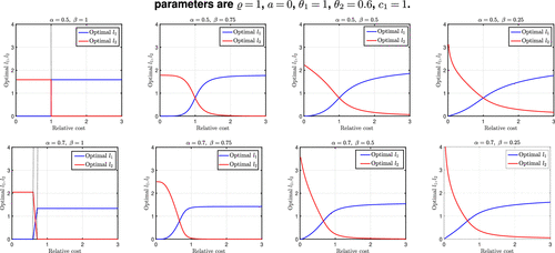
Note. The parameters are , , , , and .
5.1.2. Maintenance Example.
Theorem 2 shows that when repair and preventive service are strong complements, both stages optimally receive positive effort, whereas under near substitution, resources are allocated primarily to the more cost-effective stage. Online Appendix D grounds these results in an order-of-magnitude calibration based on published operational statistics from industrial maintenance settings for assets, such as wind turbines, generators, and other heavy equipment. The calibrated parameters produce consistent qualitative magnitudes aligned with observed practices, where repair is followed by preventive service while equipment remains offline. From an operational perspective, complementarity versus substitution can be diagnosed by how improvements in one stage affect the marginal impact of effort in the other stage. Online Appendix C provides an estimation procedure for this interaction from data. This distinction has direct design implications; complementarity favors balanced effort across stages, whereas substitution supports concentrating effort in the more cost-effective stage. Online Appendix E complements the analytical results with numerical experiments demonstrating robustness; the optimal design remains stable under moderate parameter variation, and the integrated policy yields substantial cost savings relative to decentralized benchmarks.
(
At , (both stations’ decisions are identical). Moreover, does not depend on .
For all , the ratio is decreasing in (with all else equal, greater substitution means a smaller ratio). For all , the ratio is increasing in (with all else equal, greater complementarity means a larger ratio).
The optimal cost function is decreasing in (with all else equal, greater complementarity means a larger value function).
Figure 6 is an illustration of Proposition 2. At the simplest level, complementarity effectively introduces a constraint on the network; to benefit from the effort in one station, one must make greater effort in the other station. In turn, the higher the complementarity is (the smaller the value of is), the greater the optimal cost is.
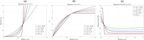
Notes. The parameters are , , , and . (a) Optimal (α = 0.7). (b) Optimal V (α = 0.7). (c) Optimal total length of stay (α = 0.7).
More subtle is the way that optimal decisions differ on both sides of the threshold . When and , part (ii) of Proposition 2 stipulates that if , the greater the complementarity is (with the relative cost fixed)—not only will more work be done (optimally) at the cheaper second station—but that relatively more is done in the second station; the relative decrease in the first station is dominated by the relative increase in the second station.
The explicitly identified value of the threshold shows that the range of costs where this happens shrinks as the first station becomes more dominant ( grows).
In Figure 6, so that threshold is per part (i) of Proposition 2 equal to . Complementarity keeps the stations as balanced as possible—as extracting value from one station necessitates keeping some effort in the other station. Accordingly, we see that as we move away from the symmetry point, it is the types with smaller that are the slowest to change (in relative terms).
This result implies that when different item types share the same relative cost but differ in their substitution level, it is sufficient to know on which side of the threshold the relative cost falls to effectively allocate efforts between the stations.
Improving Station 2 to render it a better substitute for Station 1 would have different effects on different items. Two item types that share the same relative cost might receive relatively more effort in one station depending on where items’ costs stand relative to their respective thresholds.
5.1.3. Total Processing Time.
Panel (c) of Figure 6 presents the total processing time (i.e., including all visits and both stations) for different values of . Because per item type, the rework likelihood is at optimality constant, the total processing time is proportional to a single visit length (except the first visit if ). As the cost of the second station increases, the processing time initially decreases, but then, it may increase as Station 2 becomes prohibitively expensive; this latter increase is more pronounced when complementarity is high. Like the ratio , the effect of complementarity is different (and reversed) on the left and right of the threshold.
Importantly, there is a point of relative cost (on the right of the threshold) where the processing time is minimized. Recalling that (optimal) rework is constant within an item type, this is the “sweet spot.” It achieves the optimal processing time and rework likelihood.
5.2. The Capacitated Problem
When capacity is finite ( in Problem (10)), the choice set is an intersection of the attainable workload region and the subspace defined by the constraints; see Figure 7.
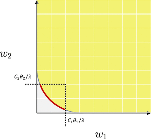
Note. The optimal solution to the cost optimization problem lies on the marked curved boundary portion.
Let us define the rate-normalized capacities
For the constrained optimization problem to be feasible, it must be that
Theorem 3 characterizes the optimal capacitated solution, which is based upon the uncapacitated solution.
(
The Lagrange multipliers capture the value of increasing the capacity. Because they are explicitly specified, we can analyze the effect of complementarity/substitution on them. To that end, let be such that . Recall that this point does not depend on and is given by . The following is a direct consequence of Proposition 2.
Fix and , which are feasible at , for some .
If , then increases with , whereas and decrease with ; the monotonicities reverse if .
If , then decreases with , whereas and increase with ; the monotonicities reverse if .
This result has an intuitive interpretation that is best understood by considering the extreme case of complementarity. As , . Thus, if , it is infinitely more valuable to increase than it is to increase . The best is when the two are equal. Extending this logic informally to any , the intuition is that we want to “balance” the line. The greater the substitution is, the more that we can realize the aforementioned value because it is costless to transfer work from Station 2. If, however, there is strong complementarity, in order to extract value in Station 1, we must keep some work in Station 2. Hence, we get less value from increasing the capacity ( is increasing in ). When , this logic is reversed.
When the capacity in Station 1 is small, the more substitution that we have, the more we want to transfer work to Station 2 (hence, we “make” Station 2 cheaper by reducing ). Complementarity, on the other hand, would mean keeping Station 2 expensive to make sure that we keep enough work in Station 1.
5.2.1. Maintenance Example.
When repair capacity is limited, the system must rely more heavily on preventive service to maintain quality, increasing the overall workload. If repair and preventive service are strong complements, however, this adjustment is less effective; restricted repair capacity reduces the value of subsequent preventive work and leads to sharper performance deterioration. The calibrated results in Online Appendix D.1 illustrate this mechanism. When repair capacity decreases from 10 to 6 workers, the system compensates by increasing preventive effort, but this adjustment yields smaller gains under strong complementarity. In complementary systems, the effectiveness of preventive service depends on sufficiently thorough repair; thus, limited capacity at the repair stage reduces the overall benefit of both stages. By contrast, when the stages are more substitutable, effort can be shifted more flexibly toward preventive service, resulting in smaller efficiency losses.
5.3. Multiple Types
In many practical systems, items differ in their characteristics, leading to heterogeneity in costs, processing rates, and complementarity levels. In this section, we generalize the analysis to incorporate multiple types of items flowing through the two stations. When resources are scarce, the different item types “compete” over them. Let be the set of item types; we expand the notation by adding the superscript k for type k. Thus, for example, is the initial quality of type k jobs, is the rate of improvement for type k jobs in Station , is the station-importance coefficient for type k items, and is the substitution/complementarity coefficient.
Let the total arrival rate to the system be , and let denote the fraction of arrivals of type k so that the arrival rate of type k items is with . Each type k is characterized by a pair of station thresholds . We denote by the collection of all type-specific threshold pairs, which we represent as a stacked 2K-dimensional decision vector. We represent as an element of .
The attainable workload region for type k is
Given a decision vector , we let , , denote the total load on Station i:
As in the case of a single type, the set is “increasing” in the vector of complementarity/substitution levels under the standard partial order; for and such that for all .
In words, the greater the complementarity is between the stations, the greater the capacity is that is needed to serve everyone. Scarce capacity introduces an interaction between item types. One must prioritize the capacity usage of the two stations, and one expects that all item types will be allocated less aggregate effort, with some “suffering” more than others. Beyond aggregation, scarce capacity also alters the effort allocation between the stations, and this reallocation differs across item types depending on their characteristics.
The total cost for K types of items with different characteristics is
The multitype constrained optimization problem is, therefore,
This problem can be equivalently expressed using the space of attainable workloads as
Theorem 4 establishes that the solution structure for each type remains as in the single-type problem but with a scaled cost ratio determined by the type-specific holding costs and by which the station’s capacity constraint is binding.
(
The dual variables and for the resource constraints scale the effective cost ratios up or down. If the capacity of Station 1 is strictly binding but Station 2 has positive slack (so ), the relative cost is reduced for all item types. The first (second) constraint if binding (hence, ()) decreases the processing time in Station 1 (Station 2) of all item types.
With , the optimal processing time in Station 1 (Station 2) for type k declines as the corresponding constraint becomes more binding. With , the scaled relative cost can drive certain item types to a regime where it is optimal to perform all processing in only one of the two stations. This is because supports three operating regimes, and there exist effective second-station costs for which it is optimal to use only a single station; recall Theorem 2, and see the example further below.
For given , , and , the optimal processing time in Station 1 decreases more (relative to the unconstrained baseline) for those item types with smaller (larger) marginal Station 1 (Station 2) costs, (). This is because effectively represents a discount in the relative Station 2 (Station 1) cost. For this same reason, two item groups, say a and b, with unconstrained solutions satisfying might have . This means that the “discount” is more significant for type a. With and , such a “swap” can still occur because of differences in substitution/complementarity. For a group with a higher degree of substitution (i.e., ), a large Station 2 discount shifts more effort toward Station 2.
5.3.1. Maintenance Example.
Consider a system that handles multiple categories of equipment that differs in maintenance costs and in how strongly repair and preventive service complement each other. When capacity is scarce, items with stronger complementarity between the two stages (lower ) retain relatively more repair effort because cutting repair capacity sharply reduces the effectiveness of subsequent preventive service. By contrast, for items that are more substitutable, the system can shift a greater share of work toward preventive service without a substantial loss in performance.
For more on the role of complementarity and substitution, Figure 8 provides two numerical examples. We consider different levels of substitution/complementarity. When there is enough capacity, all items receive their required effort mix. As capacity becomes scarce, processing time in Station 1 decreases, and processing time in Station 2 increases. When , the efforts in both stations are the same; for all (i.e., regardless of the value of ). When , the stronger the complementarity is (smaller ), the larger the ratio is. That is, items with stronger complementarity are prioritized (stay longer in Station 1 and stay shorter in Station 2) over items with a smaller level of complementarity. This is because it is easier for types with greater substitution (larger ) to compensate for the shorter processing time in Station 1 by moving effort to Station 2. Furthermore, only under substitution can we reduce to zero and provide all of the required processing in Station 2. Indeed, when (if ) and (if ), we see that under perfect substitution (). Under complementarity, we must keep the items even for a short period of time in Station 1. Note that when (if ) and (if ), under perfect substitution; the entire service is provided in Station 1.
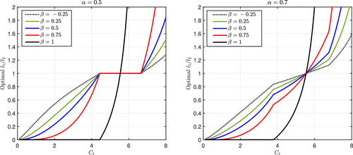
Notes. The parameters are , , , , , and . For in this example, capacity is binding if and/or ; for , it is binding at or .
In Online Appendix B.4, we consider the case where resources can be shared between the stations. In this case, the individual-station constraints are replaced with a total consumption constraint . In that setting, the interesting question is how the total capacity is optimally allocated between the stations. In Online Appendix B.5, we consider the throughput maximization problem.
6. Synthesis: The Operations Frontier
The key forces that our model seeks to capture are present in processing networks, where there is a clear notion of repair and maintenance activities. Such systems often involve sequential tasks—repair followed by preventive maintenance while the equipment remains offline—where greater investment in the first stage restores functionality and additional preventive work in the second stage enhances long-term reliability and reduces future rework, reflecting the trade-offs captured by our model. In such systems, the planner must decide how much effort to allocate to each activity. Examples include manufacturing (where the second station represents quality assurance) and services (such as healthcare, where the second station might represent postacute care follow-up). Common to these examples is that effective operation requires allocating effort across stations and item types while accounting for process characteristics, such as cost and capacity.
The model abstracts from the specifics of particular settings to focus on the role of and interaction between cost and substitution complementarity. The goal of this section is to highlight and consolidate key insights from the model that we believe are robust across various settings.
Rework, Workload, and the Operations Frontier
A fundamental feature of the model—and the reality that it seeks to capture—is that greater effort (longer processing time) results in a higher immediate workload but has the potential to reduce total workload by minimizing returns/rework. As such, the focus (both managerially and mathematically) should be on workload rather than immediate service times.
The boundary of the attainable workload region is the operations frontier for such systems and represents the trade-off between immediate and long-term workload. This trade-off is strictly convex regardless of the level of complementarity, except in the case of perfectly symmetric contribution (), where renders the boundary linear.
From a practical perspective, the nontrivial nature of this trade-off implies that capacity exchanges are not “one for one.” Reducing capacity by at one station may require adding more than capacity at the second station to maintain the same performance level.
Operating Regimes and the Effect of Rework
There are three broad regimes: two “corner” regimes, where only one station is utilized, and an interior network regime, where both stations are (optimally) used for processing.
The optimal operating regime depends on item parameters, and as a result, different regimes may coexist within the same system. For items processed exclusively at Station 1, the release threshold from the system coincides with the transfer threshold. Conversely, items processed solely at Station 2 should be directed there immediately upon arrival.
For items exhibiting (even minimal) complementarity between stations, both stations are required. Corner regimes arise only for item types where the stations are perfect substitutes. Even in these cases, unless the relative costs are significantly skewed toward one station, the optimal solution lies in the interior regime.
Cost and Substitution Interaction: A Threshold Determines the Most Effective Station
The level of complementarity influences the optimal allocation of effort between stations. For “low” relative costs (Station 1 to Station 2), greater complementarity leads to more effort being allocated to Station 1. Conversely, for “high” relative costs, greater complementarity shifts effort toward Station 2. “Low” and “high” costs are defined relative to a threshold determined by relative contribution and substitution/complementarity levels.
This threshold marks the point where the “most effective” station transitions from Station 1 to Station 2. Below this threshold, increasing interdependence between stations (through greater complementarity) results in more effort being directed to Station 1. Above the threshold, additional effort is allocated to Station 2.
The Effect of Capacity: Shifting the Threshold
Finite capacity alters the relative costs between stations. A tighter constraint at Station 1 raises its relative cost. Our results suggest that capacity adjustments will shift the balance of effort depending on where item types fall relative to the adjusted threshold. For instance, if capacity at Station 1 is reduced, effort for item types near the original unconstrained threshold will shift toward Station 2.
Expanding the Model’s Coverage
Where the specifics of a setting can be incorporated as constraints—such as minimum processing requirements at Station 1—the attainable workload region remains a valuable tool for studying the optimal network configuration. As indicated in Online Appendix C, it is feasible to estimate the model parameters using standard processing-network data to inform design decisions.
7. Concluding Remarks and Directions for Future Research
The two-station integration model is in general terms a service-network design problem. The anatomy of the network translates into the allocation of work across networked stations. We take a modeling approach that captures the individual quality evolution through the network and the way in which the station-wise quality determines rework through substitution and complementarity. Optimizing effort allocation in this case means setting the transfer targets (processing times) or efforts invested in each station to minimize the total cost of operating the system; this also implies minimizing rework and its associated cost. We introduce a model that operationalizes item characteristics and subsequently, study how the latter determines the allocation of both stations’ efforts.
The baseline model can be expanded to include additional realistic features. In our model, the transfer target l does not vary from one visit to the next. In some cases, the very event of rework reveals information about the item. It then makes sense to have different transfer targets in subsequent (i.e., postindex) visits. The model can be expanded to capture more elaborate process protocols/networks.
The workload allocation is the first-order or “fluid” optimization problem. As is the case with the fluid baseline in various queueing control problem, our solution can serve as a stepping stone for the development of dynamic control policies. Our allocation of efforts between the stations provides a baseline. Building in this baseline, real-time performance can be improved by dynamically adjusting the transfer targets in response to observed workload. The optimal control would introduce state-dependent discharge or transfer actions that are perturbations of the optimal fluid decisions.
The authors sincerely thank Editor Rami Atar, the anonymous Associate Editor and three reviewers for their insightful and constructive feedback, which has greatly strengthened this work.
1 If does not depend on l, then would minimize the workload; that is, providing any service is suboptimal. Therefore, one must allow for to grow with l to have nontrivial solutions.
2 As in the single-station case, we assume that an item is “rejected” if ; it is sent directly to the second station if . Such item types become dedicated second station traffic, in which case the single-station model is to be used with initial score .
References
- (1961) Capital-labor substitution and economic efficiency. Rev. Econom. Statist. 43(3):225–250.Google Scholar
- (2012) Doctors under load: An empirical study of state-dependent service times in emergency care. Working paper, Wharton School, University of Pennsylvania, Philadelphia.Google Scholar
- (2017) Past the point of speeding up: The negative effects of workload saturation on efficiency and patient severity. Management Sci. 63(4):1042–1062.Link, Google Scholar
- (2015) Measuring the hospital length of stay/readmission cost trade-off under a bundled payment mechanism. Health Econom. 24(7):790–802.Google Scholar
- (2019) Production networks: A primer. Annual Rev. Econom. 11(1):635–663.Google Scholar
- (2025) Dynamic control of service systems with returns: Application to design of postdischarge hospital readmission prevention programs. Oper. Res. 73(4):2242–2263.Link, Google Scholar
- (2001) Causes and cures of highway congestion. IEEE Control Systems Magazine 21(6):26–32.Google Scholar
- (2012) Broadening focus: Spillovers, complementarities, and specialization in the hospital industry. Management Sci. 58(4):708–722.Link, Google Scholar
- (1996) Stability and instability of fluid models for reentrant lines. Math. Oper. Res. 21(1):115–134.Link, Google Scholar
- (2022) Production networks and firm-level elasticities of substitution. Working paper, World Bank, Washington, DC.Google Scholar
- (2003) Correction: Brownian models of open processing networks: Canonical representation of workload. Ann. Appl. Probab. 13(1):390–393.Google Scholar
- (1997) Dynamic control of Brownian networks: State space collapse and equivalent workload formulations. Ann. Appl. Probab. 7(3):747–771.Google Scholar
- (2021)
Econometric estimation of the “constant elasticity of substitution” function in R: The micEconCES package . Hashimzade N, Thornton MA, eds. Handbook of Research Methods and Applications in Empirical Microeconomics (Edward Elgar Publishing, Cheltenham, UK), 596–640.Google Scholar - (2007) Operations systems with discretionary task completion. Management Sci. 53(1):61–77.Link, Google Scholar
- (2009) Measuring the impact of rework on construction cost performance. J. Construction Engrg. Management 135(3):187–198.Google Scholar
- (2009) Rehospitalizations among patients in the medicare fee-for-service program. New England J. Medicine 360(14):1418–1428.Google Scholar
- (2023) Characteristics of 30-day all-cause hospital readmissions, 2016–2020. HCUP Statistical Brief No. 304, Agency for Healthcare Research and Quality, Rockville, MD.Google Scholar
- (2009) Impact of workload on service time and patient safety: An econometric analysis of hospital operations. Management Sci. 55(9):1486–1498.Link, Google Scholar
- (2012) An econometric analysis of patient flows in the cardiac intensive care unit. Manufacturing Service Oper. Management 14(1):50–65.Link, Google Scholar
- (2015) Substitution elasticities in a constant elasticity of substitution framework—Empirical estimates using nonlinear least squares. Econom. Systems Res. 27(1):101–121.Google Scholar
- (2024) Systematic review and meta-analysis of the financial impact of 30-day readmissions for selected medical conditions: A focus on hospital quality performance. Healthcare 12(7):750.Google Scholar
- (1993) Re-entrant lines. Queueing Systems 13(1):87–110.Google Scholar
- (2023) Channel management in outpatient care: Implications of telemedicine and transportation support. Preprint, submitted April 12, http://dx.doi.org/10.2139/ssrn.4383199.Google Scholar
- (2000) Quantifying the causes and costs of rework in construction. Construction Management Econom. 18(4):479–490.Google Scholar
- (2000) An M/G/1 queue with second optional service. Queueing Systems 34(1):37–46.Google Scholar
- (2017) Estimation of parameters of constant elasticity of substitution production functional model. IOP Conf. Ser. Materials Sci. Engrg. 263(1):042121.Google Scholar
- (1995) Microeconomic Theory, vol. 1 (Oxford University Press, New York).Google Scholar
- (2005) Positive vs. negative externalities in inventory management: Implications for supply chain design. Manufacturing Service Oper. Management 7(1):58–73.Link, Google Scholar
- (1967) A two-level constant-elasticity-of-substitution production function. Rev. Econom. Stud. 34(2):201–218.Google Scholar
- (1973) On the elasticities of substitution and complementarity. Oxford Econom. Papers 25(1):44–56.Google Scholar
- (2006) A review of research on cost of quality models and best practices. Internat. J. Quality Reliability Management 23(6):647–669.Google Scholar
- (2021) Timing it right: Balancing inpatient congestion vs. readmission risk at discharge. Oper. Res. 69(6):1842–1865.Link, Google Scholar
- (2012) Specialization and variety in repetitive tasks: Evidence from a Japanese bank. Management Sci. 58(6):1141–1159.Link, Google Scholar
- (2011) Elasticities of substitution and complementarity. J. Productivity Anal. 36(1):79–89.Google Scholar
- (2014) When does the devil make work? An empirical study of the impact of workload on worker productivity. Management Sci. 60(6):1574–1593.Link, Google Scholar
- (2010) Intermediate Microeconomics: A Modern Approach (W. W. Norton & Company, New York).Google Scholar
- (2021) Managing discretionary services: A review and research opportunities. J. Systems Sci. Systems Engrg. 30(1):1–16.Google Scholar
- (2005) Costing the ambulatory episode: Implications of total or partial substitution of hospital care. Australian Health Rev. 29(3):360–365.Google Scholar
- (2024) Managing queues with reentrant customers in support of hybrid healthcare. Stochastic Systems 14(2):167–190.Link, Google Scholar
- (2026) An operational view on managing mass trauma events. Manufacturing Service Oper. Management 28(1):76–99.Abstract, Google Scholar
- (2026) Optimal call-in policies under travel-induced risk: Application to hybrid hospitalization. Queueing Systems 110(1):6.Google Scholar