A Storage Process with Alternating Lévy Input
Abstract
In this paper, we study a queueing process for which the dynamics are changed once the workload in the queue exceeds a predefined threshold, and these new dynamics stay in force until the queue is emptied, at which point the previous dynamics are again reinstalled. For general spectrally positive Lévy processes in each case, we derive expressions for the workload at an independent exponentially distributed random time horizon and study in detail properties of the workload in stationarity. We work out explicit formulas as well as expressions for the optimal changing threshold for special cases of the underlying process dynamics and a chosen set of involved switching, holding, and service cost functions.
Funding: The research of O. Boxma and M. Mandjes has been partly funded by the Nederlandse Organisatie voor Wetenschappelijk Onderzoek Gravitation [Project Networks, Grant 024.002.003]. The research of O. Kella is partially funded by Israel Science Foundation [Grant 3336/24] and the Vigevani Chair in Statistics.
1. Introduction
The stochastic modeling of storage and queueing processes and the derivation of distributional properties of concrete quantities like their workload or the length of their busy periods have a long history in applied probability. Over the years, many model variations were investigated and systematically understood, and nowadays, there is quite a detailed body of tools and techniques for their study available (see, for instance, Asmussen (2003) for a survey). It turned out that for various queueing models, there is an interesting and fruitful duality with models for the surplus process of an insurance portfolio that have been studied in insurance risk theory (Asmussen and Albrecher 2010, Mandjes and Boxma 2023). In particular, model assumptions on the arrival process of customers in a queue (or items in the storage process case, respectively) and the arrival process of claims in the insurance portfolio case have similar motivations and applicability, and an analogous statement holds for the random service requirements of a new customer (size of a newly arrived item in the storage facility, respectively) and the random claim sizes in the insurance model. More than that, the viewpoint of one discipline sometimes also leads to new results or simpler proofs in the other (Albrecher and Boxma 2004, Albrecher et al. 2009). Along that line, whenever some model variation in one field leads to an amenable analysis, there is a good chance that in the other field there is also an interesting analogue or some interpretation and additional insight to gain.
In the present paper, we take up on this entanglement of queueing/storage and risk theory and investigate a storage model that is motivated by a model variant recently studied in insurance risk theory. In the context of dividend payments of an insurance company, Albrecher et al. (2018) studied the ruin probability and expected discounted dividend payments for a situation where dividend payments cannot decrease over time. Concretely, Albrecher et al. (2018) assumed that once during the lifetime of the process (i.e., before the surplus is depleted, which refers to the event of ruin of the company), the rate of dividend payments can be raised permanently and the question was as follows: What is the optimal threshold to do so? Such an assumption is motivated by the fact that shareholders do not like to see a dividend rate decreasing, and it is of interest to see how much that constraint compromises the performance of the company (in terms of overall dividend payments until ruin and the resulting ruin probability). In a queueing setup, the analogous model adaptation naturally is to increase the service speed once the workload has reached a certain threshold and not reducing that speed until the queue is emptied (i.e., the workload has reached level 0 again). The motivation in that case may be that one wants to avoid too large waiting times in the queue, but the switching to and processing of an increased service speed will typically come at a cost, and, depending on the posed objective function concerning costs and benefits, there may be an optimal threshold for such a switch. In a queueing context, Cohen (1976) considered such a switching at a threshold, but in a reversible fashion; that is, once the workload goes again below that threshold, the original service speed is retaken. However, in practice this may not be feasible or efficient, for instance, because of the costs of such a switch.
Motivated by the above considerations, in this paper, we study a considerably more general model: We consider a spectrally positive Lévy process, in which the entire dynamics (the Laplace exponent of the Lévy process; in a queueing setting this could mean service speed, arrival rate of customers and service time distribution) is switched once a threshold is surpassed, and the new dynamics stay in force until the process reaches level zero. We derive results on the resulting workload, both at an exponential time horizon and in stationarity. We establish a number of other new fluctuation results along the way. The model with only the service speed changing at the switching time is contained as a special case in the above results. For the latter variant and the special cases of the two Lévy processes to be Brownian motions or compound Poisson processes with phase-type claims, we work out explicit formulas. For any given holding costs, switching costs, and service costs, we then derive expressions for the aggregate costs associated to each switching level, which allows also to identify the switching level that minimizes these costs. Finally, we illustrate the obtained results in some numerical examples. In the following, we summarize the literature that is most closely related to the results of this paper.
1.1. Related Literature
The queueing literature contains a large number of papers in which arrival rates, service time distributions, and/or service speeds change when certain thresholds are crossed. We refer to Dshalalow (1997) for an extensive survey with 277 references. An important distinction is whether (Category 1) the service speed, and so on, only depends on the present workload level or (Category 2) also on the mode of the system. In the latter category, the system switches from mode 1 to mode 2 when the workload up-crosses some level, and switches back to mode 1 at the first subsequent down-crossing of some other level (notice that if these levels are the same, then we are back in Category 1). Some early references for Category 1 are Cohen (1976) and Gaver and Miller (1962). Gaver and Miller (1962) present a pioneering study on queueing systems in which the workload determines the service speed. Cohen (1976) considers an M/G/1 queue in which the server speed is increased as soon as some workload level b is exceeded and is switched back to the original speed once b is down-crossed again (see also Tijms 1975). Cohen determines the switching level that minimizes a certain weighted sum of holding, switching and fast-serving costs.
Some references for Category 2 are Bae et al. (2003), Barlev and Perry (1993), Bekker (2009), Lee and Kim (2006), and Tijms and van der Duyn Schouten (1978). Tijms and van der Duyn Schouten (1978) consider an M/G/1 queue with finite workload capacity K and two switchover levels and , with . If the workload up-crosses level , then the arrival rate, service time distribution, and server speed are adapted. They switch back to their original value when is subsequently down-crossed. The focus in their paper is on cost minimization. Bae et al. (2003) also study cost minimization for a finite dam. The papers of Barlev and Perry (1993) and Lee and Kim (2006) are devoted to queues in which the service speed is some workload-dependent function in mode i, . The paper that is closest to ours is Bekker (2009). He considers a reflected spectrally positive Lévy process with two modes 1 and 2, with the Laplace exponent of the driving Lévy process being in mode i, . The control rule is the same as specified above. Bekker determines the steady-state workload level in this system; he also devotes some attention to the case of a finite dam, which gives rise to a doubly reflected spectrally positive Lévy process.
In several papers, service speed switching is only allowed at specific instants different from the actual instant at which a workload level is crossed. In Bekker and Boxma (2007), the service speed in an M/G/1 queue is determined by the workload level at customer arrival epochs. In Bekker et al. (2008b), it is determined by the workload level at the arrival instants of an external Poisson observer. In Bekker et al. (2009), this is extended to the case of a spectrally positive Lévy input process. The latter paper also considers the case of instantaneous switching of mode (and hence of Laplace exponent of the Lévy input process) when some workload level is crossed. We finally mention Bekker et al. (2008a); it considers a reflected spectrally positive Lévy process with two switchover levels and . The Laplace exponent of the Lévy process does not instantaneously switch when is up-crossed, but only after a random delay. If, after that delay, level zero has already been reached, then the Laplace exponent does not change. In Bekker and Boxma (2007) and Bekker et al. (2008a, b, 2009), the steady-state workload distribution is derived.
In the insurance literature, the dual model to switching the Lévy dynamics whenever a threshold level is crossed is the so-called refraction model, where dividends are paid at a certain rate above a particular surplus level (the threshold), and no dividends are paid below that level (Gerber and Shiu 2006a, and in full generality, Kyprianou and Loeffen 2010). Concretely, dividend payments reduce the increase of the surplus processes through premiums, so that the difference of the dynamics above and below the threshold is typically only in terms of the drift. In fact, such a refraction strategy is known to be optimal among all admissible dividend payout strategies in the sense that it maximizes the expected discounted dividend payments until ruin (see Jeanblanc-Picqué and Shiryaev (1995) and Asmussen and Taksar (1997) for a proof in the diffusion case; Gerber and Shiu (2006b) for a compound Poisson model; and Loeffen (2008) for the general spectrally one-sided Lévy model). A situation where the entire Lévy dynamics change at a crossing of a threshold does not have an immediate interpretation in terms of the dividend application and has, to the best knowledge of the authors, not been studied in the insurance literature.
The permanent and irreversible increase of the dividend rate at a threshold (as studied for the first time in Albrecher et al. (2018)), which motivates the queueing model of this paper, was further extended to discretely many switching thresholds in Albrecher et al. (2020) for the compound Poisson model and in Albrecher et al. (2022) for a Brownian surplus process (which is referred to as ratcheting of dividend payment rates). Using these discrete grids as building blocks, in these papers, the general continuous stochastic control problem of optimal switching thresholds and their rate increases to maximize the expected discounted dividends under this ratcheting constraint was solved (see Gao and Yin (2023), Guan and Xu (2024), Sun and Zhu (2026), and Wang et al. (2025) for recent variants and extensions).
The remainder of the paper is structured as follows. Section 2 introduces the model considered in this paper, together with notation and some preliminaries. Section 3 derives an explicit expression for the workload in this model at an exponential time horizon. Subsequently, Section 4 establishes results for the Laplace transform of the workload distribution in stationarity and gives an interpretation in terms of a decomposition result. Section 5 then translates the formulas into more explicit results for the particular cases where the Lévy processes are Brownian motions and compound Poisson processes with phase-type distributed jumps. Section 6 looks into concrete objective functions for optimizing the threshold level, given a certain structure of switching costs, holding costs, and costs for maintaining the higher service speed. Finally, Section 7 contains some concluding remarks and suggestions for future research directions.
2. Model, Preliminaries, and Notation
In this section we formally define our model, present some helpful preliminaries, and introduce useful notation. Throughout our paper the symbol abbreviates distributed, or distributed like, and LST stands for Laplace-Stieltjes Transform. Also, denotes the indicator function of the event A. We use a.s. and iff to abbreviate almost surely and if and only if, respectively.
2.1. Model
The model we study in this paper can be seen as a workload process of a storage system (Prabhu 1998) that is alternatingly driven by the two processes and (that are such that ). The workload process, to be denoted by , is affected by an underlying mode process in the following way.
The mode process J can attain two modes: + and −. We start by considering the case that ; we later discuss the case . Let for a threshold that is held fixed throughout our analysis. We define Q as the reflection of at zero until it crosses level b for the first time. This concretely means that we set (Asmussen 2003, section IX.2)
At the mode becomes −, which entails that the process Q switches its behavior to that of , and continues this behavior until it hits zero. More precisely,
At the mode becomes +. From that point, the process regenerates, and the same procedure is repeated indefinitely. This gives rise to the following recursive mechanism that is illustrated by Figure 1.
○ While J is in the + mode for the -st time, we have the following dynamics: The workload process is defined via
for , withAt time the mode switches from + to −: we put
○ Likewise, while J is in the − mode for the kth time, the workload dynamics are defined as follows:
for , withAt time , the mode switches from − to +: We put .
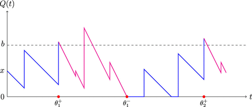
Notes. The red dots indicate mode transitions: at times the mode switches from to , at times from to . While in the mode, the workload process behaves as the reflected version of (blue segments), whereas while in the mode, the workload process behaves as (magenta segments).
It is now also clear how to define the process in case and : In that case, the process Q first behaves as until it hits level 0 and then alternates to the + mode where it behaves as the reflected version of , and so on. Clearly, the process is Markovian.
Thus far, we have not specified the driving processes and yet. In this paper, these will be assumed to be spectrally positive Lévy processes—that is, Lévy processes with no negative jumps. We exclude the case in which these processes are subordinators (i.e., almost surely nondecreasing), because in that setting there would be no reflection in mode +. Also, we assume that is not a nonincreasing linear drift, because this would lead to .
Let us first briefly introduce this class of processes and recall several useful known results.
2.2. Preliminaries on Spectrally Positive Lévy Processes
In this section, we (i) define the class of Lévy processes that we use in this paper, (ii) discuss the corresponding reflected versions to be interpreted as Lévy-driven workload processes, (iii) present a number of useful fluctuation-theoretic identities, and (iv) recall a result on the exceedance time of a Lévy-driven workload process.
2.2.1. Spectrally Positive Lévy Process.
Assume that is a spectrally positive Lévy process, that is, a Lévy process with no negative jumps (Bertoin 1998, Kyprianou 2013). Throughout, we assume . The Lévy process is characterized via its Laplace exponent . Indeed, for each we have that , where, for constants c and , and a (Lévy) measure on such that ,
It is noted that is a convex (therefore continuous) function on with . X is not a subordinator (i.e., a nondecreasing Lévy process) iff . Also, X is a subordinator iff , and . In this case,
Therefore, when X is not a subordinator, which in this section is assumed without further mention, then either is strictly increasing on or it first decreases to a negative value and then increases to infinity. For each , we denote by the right-inverse of :
2.2.2. Lévy-Driven Workload Process.
We proceed by introducing the concept of a Lévy-driven queue, which can be seen as the Lévy process reflected at zero. To this end, we define (Asmussen 2003, section IX.2)
2.2.3. Fluctuation-Theoretic Identities.
Let be an exponentially distributed random variable with mean , independent of the Lévy process X. Denote by the expected value when it is assumed that . Now consider the following three stopping times:
Define
Directly from the definition of the Laplace exponent, we have
Now consider the hitting time of level 0, by (6) written as , as a function of the initial value . As can be found in Kyprianou (2013, section VIII.1), is a subordinator with Laplace exponent , so that
See, for example, Asmussen (2003, corollary IX.3.4). This result can be considered as the generalized Pollaczek-Khinchine formula.
2.2.4. First Passage Time of a Lévy-Driven Workload Process.
We finally discuss an LST involving the reflected process at the first passage time . It identifies the joint LST of the value of the reflected process the first time it exceeds b, jointly with the time that this happens. The object of interest is thus
Here, the last equality can be verified by direct computation. In Avram et al. (2004), this object was expressed in terms of a general class of scale functions (see also Kyprianou 2013, theorem VIII.10). The precise form is not relevant in the context of the present paper; later in this work, we argue that in special cases it can be evaluated in explicit terms.
2.3. Notation
Throughout our analysis, we assume that the processes are spectrally positive Lévy processes, which are not subordinators and start at zero, and is not a deterministic nonincreasing drift, having Laplace exponents with right-inverses We also put
We define and as and , respectively, but then with respect to rather than X. Likewise, we define and as and , respectively, but then with respect to rather than X.
We will employ and to denote the probability and expectation conditional on and (where if and if ).
We will use the notations and only when Q appears, and otherwise, the qualifiers will not appear. For example or as opposed to or . Also, when in addition the starting point is not relevant or we discuss some general result, then, as already done earlier, we will write without any upper or lower index.
3. Workload at an Exponentially Distributed Time
The objective of this section is to identify the LST of the workload at an independently sampled exponentially distributed time, for each of the two possible initial modes, starting at workload level x. Indeed, we succeed in expressing
It is noted that the LST is effectively a double transform because it can be written as
By Laplace inversion (Abate and Whitt 1995), one can thus numerically evaluate the density of when has been determined. In particular the techniques developed in Den Iseger (2006) lend themselves to multidimensional Laplace inversion; see Asghari et al. (2014) and Den Iseger et al. (2013) for more specific implementation guidelines.
The following straightforward fact is the starting point of our analysis.
Let Y be a regenerative process with first regeneration time and let be a delayed regenerative process with first regeneration time , such that . Then, for being exponentially distributed with mean , independent of everything else, we have that
The proof of this lemma is elementary. The second term on the right of the top equation represents , which is seen to equal upon observing that
It is also directly seen that the top equation becomes the bottom one when . The second equality in (13) is a direct consequence of the identity . □
We note that Lemma 1 remains valid when or are not a.s. finite and the definitions of regenerative and delayed regenerative are extended. That is, only on (, respectively) the process regenerates at time (, respectively,) and its future is independent of the past.
It is directly seen that the system regenerates at times when the mode switches from − to +, which brings us into the setting of the above lemma. In the sequel, we simply write for the LST for the (nondelayed) regenerative process, that is, the process starting at time 0 at workload level 0 and being in mode +. In the remainder of this section, we determine these quantities. We break up the underlying computations into the following two steps.
(i) The simplest case is the one in which we start from some workload level in the minus mode. Then until the beginning of a new regeneration epoch the process behaves like starting from x, after which it behaves like Q starting from zero (which corresponds to the nondelayed case). Therefore, by (12) in Lemma 1,
(14)where the second equality reflects that on the process Q behaves as . By (7), we have that the first term on the right-hand side equals , and by (8), the third term equals , so we are left with evaluating the second term. Also, because by the spectrally positive nature of the process , it follows by the memoryless property of and the strong Markov property for that(15)Upon combining the above findings, we conclude that, for ,
(16)whereas for , Bernoulli-l’Hôpital’s rule implies that the first term on the right-hand side becomes .(ii) Consider now the case in which we start from some workload level in the + mode. Then, because Q behaves like until time , by the memoryless property for and the strong Markov property of the process , we have that
(17)To identify the terms on the right-hand side, we start by observing that the first term can be rewritten as
(18)From (9), the first term on the right-hand side of (18) is
(19)Again using the fact that is exponentially distributed and relying on (9) and (11), the second term on the right-hand side of (18) is seen to equal
(20)(21)We are left with evaluating the second term on the right-hand side of (17). By (16), it equals
(22)Now inserting all derived expressions into (17), we arrive at
(23)The last step is to identify the LST that corresponds to the nondelayed regenerative process Q (i.e., the one starting from workload level zero and the plus mode). Inserting in (22), the left-hand side of (23) is , which can then be solved from the equation. This eventually leads to the following expression: For , with ,
(24)It is noted that inserting into (24) provides a nice sanity check: We obtain the well-known expression
see, for example, Kyprianou (2013, section VI.5.2).
We noticed that the process regenerates at subsequent epochs where the mode process J switches from − to +. The above computations implicitly reveal the LST of the time until a new regenerative cycle begins, starting from in the plus mode:
In particular, denotes the LST of a regeneration cycle. This means that can be interpreted as the probability that such a regeneration cycle is larger than the exponentially distributed random variable . Note that, thus far, there was no need for an assumption that ensures that the time until regeneration is a.s. finite.
We now state the conclusion of the above lines of computations.
Assume that is not a subordinator. Then is given by (24), for any ,
Observe that for , we can identify by a straightforward application of the Bernoulli-l’Hôpital rule; we omit the details.
Upon inspection of the proof underlying Theorem 1, it is readily verified that it is possible to derive more refined results. For instance, one can provide an expression for (starting at workload level and the mode being +) the joint LST of (i) the value of Q at the first time J switches from + to −, (ii) this first time J switches from + to −, and (iii) the length of the subsequent interval in which the mode was −. With the parameters , , and corresponding to these random variables (i), (ii), and (iii), respectively, this LST can be written as
We have ruled out the case that is a subordinator. However, it can be observed that our analysis extends naturally to this setting. The only two necessary modifications are as follows.
Replace the expression for found in Avram et al. (2004) by its analogue in which the scale functions are substituted by the corresponding potential (renewal) measures; see, for instance, Kyprianou (2013, exercise 5.7) (with the parameters and being swapped).
In order to obtain the counterparts of (19) and (21), apply (7) rather than (9). As a consequence, in the counterpart (19), we find only the first term, that is, the one proportional to ; the same applies to the counterpart of (21).
We also refer to Kella (1998) for a related study that considers, within this context of subordinators, decomposition results in a somewhat more general framework; notably, it allows for general positive finite-mean stopping times, rather than just .
4. The Workload in Stationarity
Whereas in Section 3 we focused on the LST of the workload at an exponentially distributed time, we now focus on its counterpart for the corresponding ergodic distribution (being the long-run average limiting distribution). In Section 4.1, we derive the LST of the stationary workload, whereas in Section 4.2, we provide an insightful interpretation of the obtained expressions.
From here on, it proves useful to denote .
4.1. LST of Stationary Workload
For any regenerative process Y with first regeneration epoch having a finite mean, such a stationary distribution always exists, and if is a random variable having this distribution then
We concentrate on the long-run average limiting distribution, thus avoiding the tedious case in which has an arithmetic distribution. Indeed, if does not have an arithmetic distribution, then has a limiting distribution as .
Recall that the process regenerates when the jump process has a transition from − to +, where it is noted that at these times the workload level is necessarily zero. We impose from now on the condition : The driving process has a negative mean. This guarantees that the regeneration time of Q starting from the plus mode from workload level zero has a finite expected value provided that . This follows by recalling that is the mean time it takes the process to hit zero when starting from level x, so that the mean regeneration time equals
The goal of this section is to identify the LST of the stationary workload, denoted by in the sequel. This LST could be found from the expression given in Theorem 1 by letting in . It is somewhat simpler, however, to follow this limiting procedure applied to as given in (24). We start by defining
Observing that due to , and in addition, recalling that , we thus find that
We have to distinguish between the cases and . In both cases, we obtain an expression for , where it is noted that the former case requires an elementary application of Bernoulli-l’Hôpital’s rule, recalling that . The following theorem states the result. Define
It is readily verified that, using the compact notation for ,
Observe that and .
Assume that are not subordinators, is not a nonincreasing drift, and . Then, for any , if (which is the case iff ), then the LST of the stationary workload is given by
There is an alternative, insightful manner to arrive at the result of Theorem 2. It separately identifies the LST that corresponds to the stationary workload conditioned on being in the + mode and that is its counterpart for the − mode.
We first analyze The starting point is the following evident identity:
Using this relation, an application of (21) yields that
Inserting gives
Now follows by sending to zero in (34). In the case that , we have
We continue by analyzing To this end, we first consider our spectrally positive negative mean Lévy process such that whenever the process hits zero it jumps by an independent (from the Lévy process, that is) random nonnegative amount distributed like some V. For such a process, the steady-state distribution is that of a convolution of two distributions. The first is the steady-state distribution of a reflected Lévy process and the other is the stationary excess lifetime distribution associated with V (Kella and Whitt 1991, theorem 4.3; Ivanovs and Kella 2013, theorem 1). Therefore, recognizing that setup, the random amount that the minus mode starts with is distributed like , the LST of the process conditioned on being in the second phase is given by
Noting that the expected time consecutively spent in the + mode is , and its counterpart in the − mode is
Because by (31) the denominators are , it is consistent with the result found in Theorem 2.
Bekker (2009) considers the same model, except that his process switches from the + mode to the − mode when a threshold is up-crossed, and it switches back to the + mode when a threshold is down-crossed (extending Cohen’s model (Cohen 1976) where ). He only considers the stationary workload distribution. Using a martingale approach, he expresses that distribution, for both modes, into scale functions.
4.2. Interpretation via a Decomposition Result
In this section, we provide an interpretation of the form of in the case that , as given in (35). It follows from a fairly general decomposition result, which we present below. In the setup considered in this section, we let W be a reflected Lévy process associated with a nondeterministic spectrally positive Lévy process X having a Laplace exponent that satisfies .
Defining , because , we have that implies that , so that cannot be infinite and c is negative. Therefore, here, nondeterministic X means that the case for and all is excluded. It thus follows that Lemmas A.1 and A.2 imply that are both finite (and clearly positive), where .
Suppose that
○ M has the stationary distribution associated with W (see (10)),
○ has the stationary distribution associated with the regenerative process that behaves like W until time and then restarts from zero at time ,
○ has the excess lifetime distribution of , that is, it has the density
and LST,(39)○ has the stationary distribution of the waiting time and virtual waiting time of an M/G/1 queue with service times distributed like and arrival rate
(40)Hence, by the Pollaczek-Khinchine formula (see (10)),
(41)where(42)We are now ready to state the following decomposition result.
For every , with and being independent,
We define a regenerative cycle in the following way. We start at a time that the workload level is zero, and we end at the first time after at which the workload is zero again. This cycle can be broken into two parts: a part until time and a part from time until the workload hits zero, having expected lengths and .
By regenerative theory, recalling (42), the long run fraction of time W spends at a pre- part is .
○ The ergodic distribution of the regenerative process restricted to pre- parts is that of .
○ The ergodic distribution of the regenerative process restricted to post- parts is the distribution of a Lévy process with additional independent and identically distributed jump inputs distributed as whenever the process hits zero. It is distributed as , where M and are independent (Kella and Whitt 1991, theorem 4.2).
The ergodic distribution of the regenerative process W in its first regenerative cycle is just the ergodic distribution of W, which is that of M. Therefore,
From (45) and (39), we have the following.
For any ,
We conclude this section by interpreting (35), which provides an expression for in the case where . Representation (35) basically is a translation of (see Theorem 3 and (45)). More specifically, it is an immediate consequence of (46) upon identifying , , , and dividing the term between large brackets in (35) by .
5. Explicit Evaluation
In our expressions, a key component is —the joint LST of the random variables and , starting from x. As mentioned earlier, in Avram et al. (2004), this LST can be expressed in terms of scale functions, which are defined via their Laplace transforms. Although scale functions are explicitly known for certain classes of spectrally one-sided Lévy processes, in general, they cannot be written in closed form in terms of the model primitives (Kyprianou and Rivero 2008, Hubalek and Kyprianou 2011, Kuznetsov et al. 2012).
In Section 5.1, we consider to belong to a class of spectrally positive Lévy processes that allow for a relatively explicit analysis. Specifically, we focus on compound Poisson (CP) processes with phase-type (upward) jumps, perturbed by Brownian motion (BM). This class is particularly relevant for two reasons: (i) phase-type random variables can approximate any nonnegative random variable arbitrarily closely (Asmussen 2003, theorem III.4.2), and (ii) any spectrally positive Lévy process can be approximated arbitrarily well by CP processes perturbed by BM (Asmussen and Rosiński 2001). In Section 5.2, we consider two special cases: the case where corresponds to just BM and the case where corresponds to just CP with exponentially distributed jumps (so that behaves as the workload in an M/M/1 queue).
5.1. Superimposed CP with Phase-Type Jumps and BM
In the case where is a compound Poisson process with phase-type upward jumps, perturbed by a BM, we are able to evaluate . The analysis relies on an application of the optional sampling theorem to the following zero-mean martingale , defined for each . Let denote the local time of at zero (recall (5)) and assume . Now insert into Kella and Yor (2017, corolloary 1), to have
Let be a probability row vector, a column vector of ones and the phase generator (a substochastic matrix with spectral radius strictly less than one). Then the tail of the phase-type distribution function associated with the upward jumps is given by for . When in addition the arrival rate of the phase-type distributed jumps is and the perturbing BM has drift and variance coefficient , then, with ,
The main idea is to apply an optional sampling theorem at the stopping time (complemented by an application of the dominated and monotone convergence theorems) to obtain the identity . We conclude that
With denoting the ith unit vector, let be the LST of our phase-type distribution when . Define as the event that b is exceeded due to a jump and that the phase of this jump at exceedance is , whereas denotes the event that b is exceeded due to creeping (i.e., due to the driving process’ Brownian component); observe that in the former case, there is an overshoot, whereas in the latter case there is not. Let be the LST of on :
We are thus left with identifying the functions . Note that can be written as the ratio of two polynomials (in ), with the degree of the denominator being d. As a consequence, can be written as the ratio of two polynomials, with the numerator being of degree and the denominator of degree d. In the case where the zeroes in the complex plane of the resulting equation are distinct, let us say , we thus obtain the following equations (which are linear in the unknown functions) from (48):
Although we above dealt with the case , we complete this section by focusing on . We also impose the requirement that to make sure that is not a subordinator, implying that b is exceeded due to a jump. It is readily checked that now can be written as the ratio of two polynomials, with the numerator being of degree and the denominator of degree d. In this case, because of the absence of the Brownian component, we have . Hence, if has distinct zeroes in the complex plane, we are to solve the system of linear equations
5.2. Special Cases
As announced, in this section, we consider the cases of corresponding to BM and to CP with exponentially distributed upward jumps (so that is the workload of an M/M/1 system).
5.2.1. BM.
In the terminology of Section 5.1, this model instance corresponds to ; the equation has two roots. Let denote the negative root and the positive root. Following the procedure outlined in Section 5.1, the linear system (49) needs to be solved; it can be written as
Solving these two linear equations with respect to the unknowns and , we conclude that, with ,
Locally abbreviating and , the roots of are, for ,
We thus arrive at, with given by (51),
We mention that (51) is consistent with Mayerhofer (2019, theorem 1) and, for the case and , with Borodin and Salminen (2015, 2.0.1, p. 361).
5.2.2. CP with Exponentially Distributed Jumps and a Negative Drift.
As mentioned, in the case corresponds to CP with exponentially distributed jumps and (negative) drift , where , the process behaves as the workload of an M/M/1 queue. We let the arrival rate equal and the mean jump size . As a consequence, according to the procedure of Section 5.1, we are to solve the linear system (50):
This system of equations was found by applying the approach presented in Section 5.1 with , , , , and . We obtain that
The two roots of
We conclude, with given by (54),
By Identity (48), we note that inserting leads to
Therefore, when , we have that , which upon substituting in (48) gives an alternative way of deriving our expression for for this case. Indeed, either from taking and in (57), or from (58), we obtain that .
6. Optimizing the Threshold
In this section, we consider, in the context of our storage process with alternating input, a threshold optimization problem. Given certain switching costs, costs for operating in the − mode, and holding costs, we pose the following question: What is the switching level for which a particular weighted sum of the long-run average costs is minimized? We assume that , to make sure that the process returns to the + mode. Throughout our analysis, we intensively apply the results that we obtained for the two special cases dealt with in Section 5.2. We first consider the case that both and are BMs and then the case that both are CP processes with deterministic drifts. In both cases, we assume that and are probabilistically identical, except that they have different deterministic drifts (to be interpreted as service rates).
There are switching costs involved with changing the service speed, costs per time unit for working fast, and holding costs per time unit for each unit of work in the system. Denote the length of an arbitrary − period by , which is distributed like . By averaging over one regenerative cycle with mean , we arrive at the following objective function representing the mean costs per time unit:
In this section, we first derive in Section 6.1 a couple of identities that are helpful in evaluating . Then, in the next two sections, we provide closed-form expressions for all quantities appearing on the right-hand side of (59) for the two special cases mentioned above. The section concludes with an analysis of the optimizing threshold .
We remark that, in Feinberg and Kella (2002), an old conjecture that D-policies are optimal for the average cost per unit time criterion in an M/G/1 queue with a removable server is proved. The cost structure there consisted of switching costs, running costs, and holding costs per unit time that is a nonnegative nondecreasing right-continuous function of a current workload in the system. This criterion means that there is an optimal policy that either runs the server all the time or switches the server off when the system becomes empty and switches it on when the workload reaches or exceeds some threshold D.
A similar result might be expected to hold under the more general setup considered in the current study. Namely, that the optimal policy considered in this section is optimal among a much larger class of policies. However, this is beyond the scope of the current paper and is left for future research.
As a reviewer suggested, instead of moving from the − to the + regime only when the inventory is depleted, one might consider performing this change when the inventory hits some level from above. This setup would of course result in a richer optimization problem where one would then want to optimize with respect to both a and b. The mathematics involved in computing various descriptive results can be expected to be of a similar nature as the ones carried out in the previous sections. However, this paper was motivated by, and was supposed to be the queueing counterpart of, the ratcheting model in a risk setup as presented in Albrecher et al. (2018). Moreover, we do not expect that the attractive simple decomposition result described in Theorem 3 would continue to hold.
6.1. Some Identities
In this section, we develop a set of general identities that we later use to evaluate the cost . Let X be a spectrally positive Lévy process with Laplace exponent . The processes W and L denote the associated workload and the local time at zero, respectively. We recall that, using the notation of (2),
We also note that (48) and (57) remain valid with the plus signs removed, with any such that replacing and with replacing . Namely,
When and , we have, as a direct application of and , that .
We start by considering the case when , implying that there is a positive root of . When and for some , we have that is finite on and converges to infinity as , then there is a negative root of . With a slight abuse of notations, in both cases, we denote this root by , remarking that here we deviate from the definition of as the right-inverse of . Inserting this root in (61) gives
Therefore, in this case, whenever there are simple expressions for both and , we can compute from
We continue by considering the case when . Supposing that can be computed, then we differentiate both sides of (61) twice, let , and subsequentially divide by . This yields
Recalling the expression for from (60), we conclude that is positive (excluding the case where X is a negative drift) and finite. Therefore, whenever there is a simple expression for and a.s., we have an expression for .
It now becomes easy to compute via (61). Whenever , we differentiate both sides twice and set to obtain
When , we differentiate three times and set to arrive at
For the BM case, is zero, so that the three numbers , , and become c, , and 0, respectively. For the CP case with jump rate , a possible drift c and jumps distributed like a positive random variable Y, these become , , and , respectively. In particular, if the jump size Y is exponentially distributed with mean , then
In particular, it will be useful to note for what follows that, for any ,
6.2. BM
In this section, we consider the case of BM with drift in mode + and in mode −. We thus have
We continue by determining the various components of the objective function given in (59).
. This quantity can be obtained from (63) for and from (64) for , where we work with the Lévy process and plug in the specific stopping time . For , we use that (with in the meaning introduced in Section 6.1), , and , to obtain
(69)For , by using (64) with (or by letting in (69)), we readily obtain
(70)An alternative approach would be to obtain by differentiating with respect to , multiplying by , and inserting , but this procedure gives rise to rather involved calculations.
. Trivially,
(71). Using (65) and (66), we obtain for that
(72)whereas for , we have(73). We have (see (37)),
(74)which yields(75)
6.3. CP with Exponential Jumps
In this section, we consider an M/M/1 queue with arrival rate , mean service requirement , and service speed in mode + and in mode −. Define . We assume , so that it is guaranteed that zero is reached in mode −. We have
We proceed by determining the various components of the objective function for this M/M/1 system with switching depletion rate.
. First of all, observe that, because of the memoryless property of the exponential distribution, with Y being exponentially distributed with mean . For , we obtain the mean length of a mode + period from (63), and using that the above expression for implies that and :
(76)For , we have but , and (64) in combination with (68) yields
(77). The mean length of the mode − period is just the mean length of an M/M/1 busy period that starts with an (exceptional) service time with mean , and hence
(78). Using (65) and (66), we obtain for that
(79)whereas for ,(80)Notice that, for , the factor in front of in the last line of (79) can be interpreted as the mean steady-state workload of a conventional M/M/1 queue (without any switching, that is) operating with service speed .
. We have (see (37)),
(81)with denoting the LST of an exponentially distributed random variable with mean . Noting that this expression is the product of the LST of the M/M/1 waiting time or workload distribution and that of the residual of , using (78), we obtain(82)
6.4. Optimal Switching Threshold
Now that we have all components of the objective function , we turn to the question of determining that minimizes .
The easiest optimization problem arises for BM, in the case that . The objective function now becomes
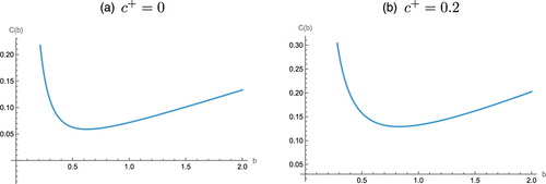
If , then one can divide numerator and denominator of by b, and it is readily seen that a unique minimum occurs for
In this expression, the effects of large or small cost coefficients and are evident. First, a large leads to a small , as expected. Second, a large results in a large . Apparently, even though the costs of operating in the − mode are high in this case, the fact that the mean duration of a mode + period is an order b larger than that of a mode − period makes it profitable to choose a large value of b (Figure 3(a)).
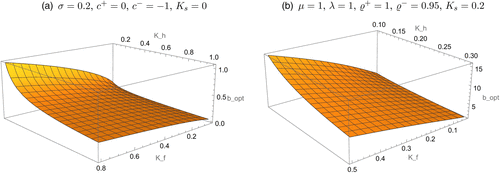
In the CP case with exponentially distributed jumps, where our process corresponds to an M/M/1-type storage system with switching service rate, the easiest optimization problem arises when . With Y denoting an exponentially distributed random variable with mean , we introduce to make our expressions more compact. The objective function now becomes
In the case of BM with , the objective function becomes
We conclude by considering the case of CP with exponentially distributed jumps and . The objective function becomes
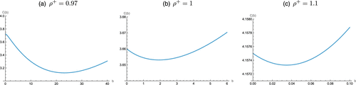
For large b, the behavior of strongly depends on the value of . If , then grows essentially linearly in b for large b. If (downward drift in the + mode), then grows exponentially for large b, so that behaves as for large b. The minimum of can be determined numerically relying on standard computational packages (Figure 4, (a) and (c)). Note how dramatically the location of the minimum changes in Figure 4 as transits through the value 1.
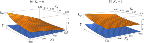
It is interesting to compare the optimal threshold with the one from Cohen (1976), where the switching to the − mode is reversible at the next down-crossing of b, so that several switches can take place during a busy period. Most of the results in Cohen (1976) are derived for the case of no switching costs (); only for the case , there is also a formula for . We therefore focus on the comparison for . Cohen (1976, equation (4.21)) gives, for Exp(1)-distributed service times, the explicit formula
7. Concluding Remarks
In this paper, we studied a queueing process with Lévy input that is modified whenever the workload process hits a prespecified threshold for the first time during a busy period, and after the queue is empty, it restarts with the original dynamics. We obtained expressions for the workload at an independent exponential time and studied the stationary workload in more detail. For a particular specification of costs for switching, holding, and increased service speed, we also derived formulas for optimal switching thresholds in the case of an underlying Brownian motion or compound Poisson process with positive jumps as Lévy input.
There are various directions in which further research could be of interest. In the paper, we assumed the holding costs to be independent of the current workload. It may be practically relevant to remove that assumption. From a mathematical perspective, this will lead to a more complicated form of (59), where the function will appear within the integrals, and it will then depend on the concrete form of the latter function whether the analysis still remains amenable. Note that Cohen (1976) allowed such costs to be a different constant below and above the chosen threshold, but the goal here would be to choose the optimal threshold given a concrete exogenous form of .
Another direction of interest may be to jointly study the choice of the threshold b and the increased service rate after upcrossing b, so that the degree of additional service becomes part of the optimization procedure. Furthermore, it could be practically relevant to only inspect the level of the workload at independent exponentially distributed epochs and switch the process only at those times in case one is in the + mode above b. One could then study the efficiency loss of not continuously observing the process.
In risk theory, the problem of increasing the dividend rate once over time was later generalized to identify the optimal schedule of when to raise the dividends continuously and by how much in order to maximize the expected dividend payments (Albrecher et al. 2020, 2022). Such a stochastic control problem could also be of interest in the present queueing application by determining the optimal schedule of raising the service speed gradually as a function of current workload relative to a given cost function. However, the mathematical techniques needed for such an approach will be quite different from the ones used in this paper. A first step in that direction could be to allow for multiple thresholds in the analysis and investigate the sensitivity of the cost function.
Appendix A. Auxiliary Results
In the following two lemmas, X is a Lévy process that is not the negative of a subordinator, W is the associated reflected process, and, for , . Note that the deterministic function ct for also counts as the negative of a subordinator (which has been ruled out).
There exists some such that for all , . In particular, has finite moments of all orders.
If X is not the negative of a subordinator, then, for any , (Sato 2005, theorem 24.11). Therefore, for some , we have that . Take such that . Then
Take (so that ) and denote
Clearly,
When, in addition, X is spectrally positive, iff
It is clear that iff
Now multiply the displayed equation in Kyprianou (2013, theorem VII.7) by u and integrate with respect to u on the interval , as well as the rest of the variables. The integration with respect to u (for fixed v) results in
Both upper and lower bounds are finite iff and hence the equivalence follows. □
References
- (1995) Numerical inversion of Laplace transforms of probability distributions. ORSA J. Comput. 7:36–43.Link, Google Scholar
- (2020) Optimal ratcheting of dividends in insurance. SIAM J. Control Optim. 58:1822–1845.Google Scholar
- (2022) Optimal ratcheting of dividends in a Brownian risk model. SIAM J. Financial Math. 13:657–701.Google Scholar
- (2018) Dividends: From refracting to ratcheting. Insurance Math. Econom. 83:45–58.Google Scholar
- (2009) The tax identity in risk theory: A simple proof and an extension. Insurance Math. Econom. 44:304–306.Google Scholar
- (2014) Numerical techniques in Lévy fluctuation theory. Methodol. Comput. Appl. Probab. 16:31–52.Google Scholar
- (2003) Applied Probability and Queues (Springer, New York).Google Scholar
- (2014) Lévy processes, phase-type distributions, and martingales. Stochastic Model. 30:443–468.Google Scholar
- (2010) Ruin Probabilities, 2nd ed. (World Scientific, Singapore).Google Scholar
- (2001) Approximations for small jumps of Lévy processes with a view towards simulation. J. Appl. Probab. 38:482–493.Google Scholar
- (1997) Controlled diffusion models for optimal dividend pay-out. Insurance Math. Econom. 20:1–15.Google Scholar
- (2004) Exit problems for spectrally negative Lévy processes and applications to (Canadized) Russian options. Ann. Appl. Probab. 14:215–235.Google Scholar
- (2003) Average cost under the policy in a finite dam with compound Poisson inputs. J. Appl. Probab. 40:519–526.Google Scholar
- (1993) Two-stage release rule procedure in a regenerative dam. Probab. Engrg. Inform. Sci. 7:571–588.Google Scholar
- (2009) Queues with Lévy input and hysteretic control. Queueing Systems 63:281–299.Google Scholar
- (2007) An queue with adaptable service speed. Stochastic Model. 23:373–396.Google Scholar
- (2008a) Queues with delays in two-state strategies and Lévy input. J. Appl. Probab. 45:314–332.Google Scholar
- (2008b) Queues with service speed adaptations. Statist. Neerlandica 62:441–457.Google Scholar
- (2009) Lévy processes with adaptable exponent. Adv. Appl. Probab. 41:177–205.Google Scholar
- (1998) Lévy Processes (Cambridge University Press, Cambridge, UK).Google Scholar
- (2015) Handbook of Brownian Motion—Facts and Formulae, 2nd ed. (Birkhäuser, Basel).Google Scholar
- (1976) On the optimal switching level for an M/G/1 queueing system. Stochastic Processes Appl. 4:297–316.Google Scholar
- (2015) Queues and Lévy Fluctuation Theory (Springer, Berlin).Google Scholar
- (2006) Numerical transform inversion using Gaussian quadrature. Probab. Engrg. Inform. Sci. 20:1–44.Google Scholar
- (2013) A Wiener–Hopf based approach to numerical computations in fluctuation theory for Lévy processes. Math. Methods Oper. Res. 78:101–118.Google Scholar
- (1997)
Queueing systems with state dependent parameters . Dshalalow JH, ed. Frontiers in Queueing (CRC Press, Boca Raton, FL), 61–116.Google Scholar - (2002) Optimality of D-policies for an M/G/1 queue with a removable server. Queueing Systems 42:355–376.Google Scholar
- (2023) A Lévy risk model with ratcheting and barrier dividend strategies. Math. Foundations Comput. 6:268–279.Google Scholar
- (1962)
Limiting distributions for some storage problems . Arrow KJ, Karlin S, Scarf H, eds. Studies in Applied Probability and Management Science (Stanford University Press, Stanford, CA), 110–126.Google Scholar - (2006a) On optimal dividends: From reflection to refraction. J. Comput. Appl. Math. 186:4–22.Google Scholar
- (2006b) On optimal dividend strategies in the compound Poisson model. North Amer. Actuarial J. 10:76–93.Google Scholar
- (2024) Optimal ratcheting of dividend payout under Brownian motion surplus. SIAM J. Control Optim. 62:2590–2620.Google Scholar
- (2011)
Old and new examples of scale functions for spectrally negative Lévy processes . Dalang RC, Dozzi M, Russo F, eds. Proc. Seminar on Stochastic Analysis, Random Fields and Applications VI: Centro Stefano Franscini (Springer, Berlin), 119–145.Google Scholar - (2004) A ruin model with dependence between claim sizes and claim intervals. Insurance Math. Econom. 35:245–254Google Scholar
- (2013) Another look into decomposition results. Queueing Systems 75:19–28.Google Scholar
- (1995) Optimization of the flow of dividends. Russian Math. Surveys 50:257–277.Google Scholar
- (1998) An exhaustive Lévy storage process with intermittent output. Stochastic Model. 14:979–992.Google Scholar
- (1991) Queues with server vacations and Lévy processes with secondary jump input. Ann. Appl. Probab. 1:104–117.Google Scholar
- (2017) Unifying the Dynkin and Lebesgue-Stieltjes formulae. J. Appl. Probab. 54:252–266.Google Scholar
- (2012)
The theory of scale functions for spectrally negative Lévy processes . Cohen SN, Madan DB, Winkel M, eds. Lévy Matters II: Recent Progress in Theory and Applications: Fractional Lévy Fields, and Scale Functions (Springer, Berlin), 97–186Google Scholar - (2013) Fluctuations of Lévy Processes with Applications, 2nd ed. (Springer, Berlin).Google Scholar
- (2010) Refracted Lévy processes. Ann. IHP Probab. Statist. 46:24–44.Google Scholar
- (2008) Special, conjugate and complete scale functions for spectrally negative Lévy processes. Electronic J. Probab. 13:1672–1701.Google Scholar
- (2006) A workload-dependent M/G/1 queue under a two-stage service policy. Oper. Res. Lett. 34:531–538.Google Scholar
- (2008) On optimality of the barrier strategy in de Finetti’s dividend problem for spectrally negative Lévy processes. Ann. Appl. Probab. 18:1669–1680.Google Scholar
- (2023) The Cramér-Lundberg Model and Its Variants (Springer, Cham, Switzerland).Google Scholar
- (2019) Three essays on stopping. Risks 7:1–10.Google Scholar
- (1998) Stochastic Storage Processes: Queues, Insurance Risk, Dams, and Data Communication (Springer, Berlin).Google Scholar
- (2005) Lévy Processes and Infinitely Divisible Distributions (Cambridge University Press, Cambridge, UK).Google Scholar
- (2026) Spectrally negative Lévy risk model under ratcheting dividend strategy and capital injections with transaction costs. Communications in Statistics-Theory and Methods 55(4):1246–1267.Google Scholar
- (1975) On a switch-over policy for controlling the workload in a queueing system with two constant service rates and fixed switch-over costs. Zeitschrift Oper. Res. 21:19–32.Google Scholar
- (1978) Inventory control with two switch-over levels for a class of M/G/1 queueing systems with variable arrival and service rate. Stochastic Processes Appl. 6:213–222.Google Scholar
- (2025) Optimal ratcheting of dividends with capital injection. Math. Oper. Res. 50:2073–2111.Link, Google Scholar