Introducing and Integrating Machine Learning in an Operations Research Curriculum: An Application-Driven Course
Abstract
Artificial intelligence (AI) and operations research (OR) have long been intertwined because of their synergistic relationship. Given the increasing popularity of AI and machine learning in particular, we face growing demand for educational offerings in this area from our students. This paper describes two courses that introduce machine learning concepts to undergraduate, predominantly industrial engineering and operations research students. Instead of taking a methods-first approach, these courses use real-world applications to motivate, introduce, and explore these machine learning techniques and highlight meaningful overlap with operations research. Significant hands-on coding experience is used to build student proficiency with the techniques. Student feedback indicates that these courses have greatly increased student interest in machine learning and appreciation of the real-world impact that analytics can have and helped students develop practical skills that they can apply. We believe that similar application-driven courses that connect machine learning and operations research would be valuable additions to undergraduate OR curricula broadly.
Supplemental Material: Supplemental material is available at https://doi.org/10.1287/ited.2021.0256.
1. Introduction
Artificial intelligence (AI) and operations research (OR) have long been intertwined because of their synergistic relationship (Bennett and Parrado-Hernández 2006). For example, Markov decision processes form the theoretical foundation for classical reinforcement learning (Bertsekas and Tsitsiklis 1996, Sutton et al. 1999) and deep reinforcement learning relies heavily on the theory of partially observable Markov decision processes (Schmidhuber 2015). Broadly speaking, both fields are concerned with using computational and mathematical approaches to improve decision making.
There are key elements of OR in AI. For example, machine learning (ML) models are typically trained by solving an optimization problem, from ordinary least squares and maximum likelihood estimation for regression models to high-dimensional nonconvex optimization problems for deep neural networks (Bishop 2006). In general, the optimization algorithms (e.g., gradient descent, combinatorial optimization, local search, meta-heuristics, etc.) used to train AI models are an integral part of an operations researcher’s toolbox (Boyd et al. 2004, Hentenryck and Bent 2009).
There are also elements of AI in OR. A common approach to solving real-world problems is a predict-then-optimize approach, where key parameters of an optimization model are predicted via machine learning, before (or at the same time as) the optimization models are solved (Elmachtoub and Grigas 2017, Mišić and Perakis 2020). For example, in vehicle routing problems, researchers often leverage machine learning models to predict travel times and subsequently use those predictions to optimize delivery routes. In inventory management, model-forecasted demand can be used as an input to various pricing or procurement models. AI has also been leveraged by the OR community to develop heuristics that can solve hard combinatorial optimization problems (Cochocki and Unbehauen 1993, Smith 1999).
Given the increasing popularity of AI and machine learning in particular (Columbus 2020), we face growing demand for educational offerings in this area from our students. Although there are options for industrial engineering and operations research (IEOR) students to learn AI concepts through courses in computer science departments, these courses tend to be less focused on OR applications and, these days, are often heavily oversubscribed. Moreover, there is limited education research literature on teaching machine learning that can be leveraged for course design, especially for non–computer science majors (Fiebrink 2019, Sulmont et al. 2019). Most of the existing education literature and teaching material is either designed for students from nonmathematical fields (Way et al. 2017) or designed for graduate level computer science students (Lavesson 2010, Mike et al. 2020). For these reasons, we believe there is value in developing application-driven courses in machine learning, tailored to the IEOR audience. These courses could focus on motivating and applying machine learning methods in IEOR applications, while also discussing the deep connection between the two fields.
In this paper, we describe two courses that we developed to introduce machine learning concepts to undergraduate, predominantly IEOR students: Analytics in Action (University of Toronto) and Machine Learning in Action (University of Wisconsin–Madison). We will present the structure and assessment methods of both courses. We also present an exhaustive list of the teaching modules covered in either course, which include topics in AI (primarily machine learning), OR, or a combination of both. Our two courses cover different subsets of these modules, and these modules can be easily adapted for use at other institutions. In contrast to many computer science courses in machine learning, our courses are less theoretical and students are not expected to develop the techniques from first principles. Students get a broader treatment of machine learning methodologies aimed at understanding how and when to apply a given technique. The course names—“X in Action”—serve to emphasize two important features of these courses: (1) the focus on real-world applications and (2) that most of the learning will be through doing, including significant hands-on coding experience.
2. Background
The first iteration of Analytics in Action, developed by the second author with the first author as a teaching assistant, was delivered at the University of Toronto (a large public research university) in January 2017. Increasing demand from industry for students with machine learning skills was the primary motivation for introducing this course. Based on anecdotal conversations, many students were developing these skills independently or learning on the job during their co-op year (typically between their third and fourth year of undergraduate studies). Our curriculum provided limited exposure to machine learning, so this course was developed to provide a broad, application-based introduction to the topic, with the goal of helping students develop basic familiarity with the material and build excitement to continue learning after the course.
At the time, it was listed as a fourth year (senior) undergraduate elective but was also open to third year students. Because many students wanted to take this course before their co-op year, and given the introductory nature of the course, the student distribution tended toward third year students over the next few years. As a result, it is now listed as a third year elective with an average enrollment of 97 students and the support of three teaching assistants. There are three prerequisites for Analytics in Action: an introductory probability/statistics course, deterministic operations research (e.g., linear and integer programming, network flows, etc.), and stochastic operations research (e.g., Markov chains, stochastic processes, etc.).
The initial course content was drawn from several different sources, with the primary sources being the course The Analytics Edge, developed by Dimitris Bertsimas at the Massachusetts Institute of Technology (MIT), and the instructor’s own research. The lectures borrowed from The Analytics Edge were designed for an in-person MBA course, although a massive open online courses (MOOC) version of the course has since been created at MIT. The corresponding textbook served as a useful reference (Bertsimas et al. 2016). “Analytics” in the course title was used to emphasize the broader nature of this course, including both predictive and prescriptive analytics. Over time, new lectures have been added, drawn from recent and novel application areas of machine learning, or the combination of machine learning and OR, published in the OR literature.
A new version of Analytics in Action, called Machine Learning Applications, that focused exclusively on predictive analytics was developed by the first author and delivered at MIT in April 2019. It was cross-listed as an elective in the master of business administration, master of supply chain, and master of business analytics programs. Interestingly, there were students simultaneously enrolled in The Analytics Edge; student feedback suggested that the courses were complementary, with the current course focusing more on machine learning, including more theoretical components, whereas The Analytics Edge included broader coverage of related topics outside of machine learning (e.g., optimization and simulation).
A revised version of Machine Learning Applications, named Machine Learning in Action, has been delivered at the University of Wisconsin–Madison (a large state research university) since September 2019. The course is listed as both a senior undergraduate and graduate elective, and enrollment is split roughly evenly between the two groups with an average of 33 total students and the support of one teaching assistant (TA). The content is similar to Machine Learning Applications but with more emphasis on the use of OR tools to train machine learning models, such as ordinary least squares and support vector machines. The required prerequisites for Machine Learning in Action are an introductory statistics course, deterministic operations research, and a Python programming course. Additional recommended prerequisites include a course on probability theory, stochastic operations research, and a course on data visualization.
3. Course Goals and Learning Objectives
In developing these courses, our goals were to
Build interest, excitement, and ultimately proficiency in machine learning.
Highlight successful and innovative real-world applications of analytics, which may motivate students to continue learning and developing their skills in this area.
Highlight synergistic connections between machine learning and operations research.
Regarding learning objectives, by the end of our courses students should be able to
Recognize problems that are amenable to analytics methods and identify whether a predictive or prescriptive (or both) analytics approach is appropriate.
Apply an appropriate analytics approach to solve a problem with real data using computer software.
Effectively communicate analytics methodology and results through written and oral formats.
In addition to learning specific methods, we want students to learn an overall approach to solving real-world problems that involves exploring data, generating hypotheses, creating and validating models, and then figuring out the “so what.”
4. Course Design
4.1. Course Structure
Both courses have in-person lectures that introduce a technical topic through a real-world example and in-person labs that focus on developing proficiency in the analytic methods used. The courses differ in how the learning is supplemented and reinforced, either through an extensive project with multiple deliverables (University of Toronto) or through homework assignments and a final exam (University of Wisconsin–Madison). Table 1 provides a high-level outline of the structure for the fall 2020 version of Analytics in Action and the fall 2019 version of Machine Learning in Action, including a breakdown of class time and assessment. The primary reason for the different course structures (and content) was instructor preference.
|

Table 1. Outline of the Course Structure for the Fall 2020 Version of Analytics in Action and the Fall 2019 Version of Machine Learning in Action
| Teaching | ||
|---|---|---|
| University of Toronto | University of Wisconsin–Madison | |
| No. of lecture modules | 12 (23 hours) | 10 (25 hours) |
| No. of labs | 11 (33 hours)a | 7 (8.5 hours) |
| No. of tutorials | 10 (10 hours)a | — |
| Assessment | ||
| University of Toronto | University of Wisconsin–Madison | |
| No. of homework | 0 | 4 (40%) |
| No. of quizzes | 6 (33.3%) | 5 (20%) |
| Final exam | No | Yes (40%) |
| Project | Yes (66.7%) | No |
aTwelve hours of laboratory time and four hours of tutorial time were used for project meetings/presentations; the remaining tutorial time was used for quizzes.
4.1.1. University of Toronto.
Machine learning is the primary focus of the course. Secondary coverage includes traditional OR topics like linear and integer optimization and simulation, with added focus on overlap with machine learning. The course is delivered over a 13-week semester. In the first half of the course, each week is a module focusing on a specific technique (e.g., linear regression, logistic regression, etc.). Each module generally consists of two lectures (two to three hours total) that follow a similar cadence: (1) describe one or two real-world applications in depth, (2) introduce the technique in the context of the application, (3) return to the application to see the results of applying the technique. Sandwiched between the two lectures is a computer laboratory (three hours) where students get hands-on coding experience, implementing the technique in the context of a similar problem as covered in the lecture, with a data set. The second half of the course includes modules on combining machine learning and OR (e.g., predict-then-optimize), guest lecturers from industry, and a few miscellaneous topics. Most labs in the second half are unstructured project time, where student teams work on their project with TAs roaming the room in support. See Figure A.1 in Appendix A for a week-by-week breakdown of the course.
Assessments in the first half of the course are primarily based on laboratory quizzes to evaluate knowledge of the introduced techniques and fluency in their use. Project deliverables are spread throughout the semester but concentrate toward the end of the semester.
4.1.2. University of Wisconsin–Madison.
Machine learning is the exclusive focus of the course, with additional emphasis on how OR methods can be used to train machine learning models. The course is delivered over a 13-week semester and includes 11 modules. The first half of the course is similar in content to the University of Toronto course, and all modules follow the structure and cadence described above. In contrast with the University of Toronto course, the second half of the University of Wisconsin–Madison course has the same structure as the first half but explores more advanced machine learning topics, such as ensembles, support vector machine, and neural networks. Aside from exploring more advanced machine learning topics, the other major difference between the courses is that the University of Wisconsin–Madison course focuses on using OR models to train the various machine learning models covered throughout the semester. Assessments, including laboratory quizzes and homework, are spread evenly throughout the semester and culminate with a final exam. See Figure B.1 in Appendix B for a detailed course outline.
4.2. Course Modules
Each course comprises a set of modules. Each module focuses on one or two real-world applications, which are used to explore a technical topic (e.g., a methodology or combination of methodologies). Each application motivates the use of the methodology and facilitates learning with respect to how the model/method was created, what data were used, and the implications/insights generated by the results. Some of the applications used in the course have changed the world (e.g., Framingham Heart Study), whereas others are new and their potential impact is not yet known (e.g., drone-delivered defibrillators). The diversity of application topics provides students with the opportunity to learn from well-established applications and think critically about the potential future impact of new ideas.
The basic structure of each module is to first introduce, motivate, and discuss the application, with a particular focus on discussing relevant analytical questions and hypothesis. Significant time is spent describing the overall application and motivation, so students build an in-depth appreciation for the real-world problem that analytics can be used to tackle. Next, we teach a technical method that can be used to answer the highlighted questions and hypothesis and discuss the insights generated by the model. Finally, we return to the application and consider the impact of analytics in the real-world context. Supplementing the lecture content is a laboratory that provides students with an opportunity to use real data to develop proficiency in the analytic methods taught.
Table 2 provides a list of all modules with details on the applications used and time spent in each course. Appendix C includes detailed descriptions for all course modules from our two courses (shown in Table 2); a single course does not include all of them. We provide the full list for potential instructors to see what such a course might include. The University of Toronto course includes both predictive and prescriptive analytics methods (linear regression, logistic regression, clustering, classification and regression trees (CART)/random forests, optimization, simulation, predict-then-optimize), whereas the University of Wisconsin–Madison course focuses exclusively on machine learning (linear regression, logistic regression, clustering, CART, ensembles, support vector machines, deep learning). Although these courses are designed for a 13-week term, they can be easily shortened by selecting fewer modules. For example, Analytics in Action.5 was taught during a six-week term, covering only linear regression, logistic regression, CART, ensembles, and deep learning. Although our courses are application driven, we list the modules below according to the technical topic because each topic can be taught with multiple applications, depending on instructor preference.
|
Table 2. Detailed Breakdown of the Course Modules
| University of Toronto | University of Wisconsin–Madison | |||||
|---|---|---|---|---|---|---|
| Module | Lecture hours | Laboratory hours | Lecture application(s) | Lecture hours | Laboratory hours | Lecture application(s) |
| Introduction | 1 | 3a | — | 0.5 | 1g | — |
| Data engineering | — | 3a | — | 1.25 | 1.25e | — |
| Model engineering | — | 3b | — | 2.5 | 1.25e | — |
| Linear regression | 2 | 3c | Moneyball, wine quality | 2 | — | Wine |
| Logistic regression | 2 | 3c | Framingham Heart Study | 2.5 | 1.25 | Framingham |
| Clustering/KNN | 2 | 3b | Hockey player types | 2.5 | 1.25 | News text analysis |
| CART/RF | 4 | 3 | Supreme Court, crime patterns, travel time | 2.5 | 1.25 | Supreme Court |
| Ensemble methods | — | — | — | 2.5 | 1.25f | Travel times, Netflix prize |
| SVM | — | — | — | 2.5 | 1.25f | ImageNet competition |
| Deep learning | — | — | — | 2.5 | 1.25 | History/future of ML |
| Linear optimization | 2 | 3d | Radiation therapy | — | — | — |
| Integer optimization | 4 | 3d | AED placement, scheduling | — | — | — |
| Simulation | 2 | 3 | Blackjack, tennis | — | — | — |
| Predict-then-optimize | 2 | 3 | eHarmony, refugee resettlement | — | — | — |
| Communication | — | 3 | — | 2.5 | — | Drone delivered AEDs |
| Wrap-up | 2 | — | — | 1.25 | — | — |
Notes. See Appendices A and B for a week-by-week course outline. AED, automated external defibrillator; SVM, support vector machine; KNN, K-nearest neighbors; CART, classification and regression tree; RF, Random forest.
a,b,c,d,e,fIndicates a joint laboratory.
gOutside class time.
4.2.1. A Detailed Lecture Outline: Predicting Travel Times in Dhaka, Bangladesh.
In this section, we provide a detailed outline of a lecture that is based on research that uses random forest to predict travel times in developing urban centers (Boutilier and Chan 2020). This lecture is included as part of the CART module (and included in a laboratory) at the University of Toronto and as part of the Ensemble module at the University of Wisconsin–Madison.
The lecture begins with a motivating example focused on the application of predicting travel times in developing urban centers as part of a larger research project that seeks to optimize ambulance location–routing decisions. The application provides an opportunity to highlight how culture differences and common challenges found in developing countries impacted the project. For example, the lack of yielding for ambulances impacts the optimization modelling approach and the lack of data availability on historical travel times required custom-built GPS devices for data collection. The application also provides an opportunity to highlight other challenges associated with GPS data collection, such as matching the GPS way-points to roads in the network.
Unlike some other topics, the application is not directly linked to a specific methodology and instead focuses on comparing various algorithms, including machine learning models and simple baseline approaches. We connect the application with random forest because it ends up performing the best. Because of the lack of direct connection, we also provide a more technical motivation for random forest by highlighting how it can be used to address CART’s tendency to overfit. The technical motivation serves as a brief recap of CART and a smooth transition to the technical component of the lecture.
The technical content focuses on describing the bootstrap aggregation algorithm and how it is used to train a random forest model. Because the students have already been exposed to CART (ideally in the last lecture), the lecture focuses on how individual CARTs are combined to create a random forest and make predictions (rather than how to train individual CART models). Aside from model training and prediction, we also highlight that feature importance can be extracted from the random forest model and used to provide some notion of interpretability.
Following the technical content, the lecture returns to the practical application. We provide a detailed exploratory data analysis and discussion on data/feature engineering (the application involves feature creation and data augmentation—see Boutilier and Chan 2020). We then describe the model training/testing setup and present a comparison of the different models. The lecture concludes by connecting the predictions back to the larger application of optimizing ambulance location–routing. The predictions provide accurate estimates for ambulance travel times throughout the road network at different times of day and days of the week and are used as input to the optimization model. Without accurate input parameters, the model may not provide accurate recommendations for how to locate and route ambulances. This integration can be connected to both the integer programming and the predict-then-optimize modules. The application also serves as motivation for how a combination of analytics techniques can be used to solve important global health problems.
The laboratory at the University of Wisconsin–Madison provides students with the real travel time data from Dhaka, Bangladesh and asks them to compare various algorithms, such as CART, random forest, and AdaBoost.
4.3. Assessment
The following subsections describe the union of the assessments used in our two courses. The assessment used in each course is tailored to its specific structure. For example, the University of Toronto course assesses students based on laboratory quizzes (one-third of the grade) and a large project (two-thirds of the grade). Laboratory quizzes are used as a check for basic understanding of the content and to ensure sufficient individual assessment is provided in the course, as required by our curriculum rules. The project is the main evaluation in the course and consists of several deliverables as described below. The University of Wisconsin–Madison course assesses students using laboratory quizzes (20% of the final grade), large homework assignments (40%), and a final exam (40%). Each quiz is paired with a homework assignment to evaluate content from two lecture modules. Students are encouraged to work in groups of two for the homework; similar to the University of Toronto course, the quizzes and exam are used to maintain individual assessment.
4.3.1. Laboratory/Laboratory Quiz.
Labs focus on developing proficiency in the analytics methods taught. Depending on the course structure, labs can be specific to a module or include topics from multiple modules. The laboratory itself is conducted via Jupyter Notebook; students are provided with clean data and a code skeleton; the one exception is a laboratory from the University of Wisconsin–Madison that focuses on cleaning messy data. They work through the laboratory, complete the code, and answer questions that are placed throughout the notebook. Labs are posted the week before, so they can do them at their own pace. The University of Toronto course has now migrated to using Google Colaboratory, which also facilitates student collaboration on the major coding tasks of the project.
Although most students had encountered Python in a previous course, that course was more focused on basic coding skills like understanding “for” loops. To improve baseline knowledge, we conduct an introductory Python laboratory at the beginning of the semester that focuses on relevant packages and skills for handling and visualizing data and preparing data for machine learning activities. We use the following Python packages: scipy (Virtanen et al. 2020), numpy (Harris et al. 2020), pandas (Wes McKinney 2010), scikit-learn (Pedregosa et al. 2011), matplotlib (Hunter 2007), seaborn (Waskom and Seaborn Development Team 2020), and graphviz (Ellson et al. 2001).
Short (20–30 minutes) laboratory quizzes are conducted at the end of certain laboratory sessions. The quizzes test technical knowledge, including conducting calculations, building simple models, interpreting model output, and understanding key model concepts and assumptions. Students who completed the laboratory notebook and worked to develop an independent understanding of the material should find laboratory quizzes to be fairly straightforward. Working with classmates on the laboratory is encouraged. However, copying and pasting code blocks without understanding them will likely lead to poor grades on the laboratory quizzes.
4.3.2. Homework.
Each homework assignment typically focuses on the material from two lecture modules. Students are encouraged to work on and submit their homework in groups of two. Each homework includes two large “coding questions” (one from each module) that provide students with real data and ask them to answer practical questions. The remaining questions are a combination of short-answer and calculation questions that focus on conceptual understanding.
4.3.3. Project.
The project is conducted in teams of four and asks students to select a real-world problem to investigate using the techniques learned in the course. In particular, students are required to (i) identify a problem or application area where analytics can be applied, (ii) obtain data and conduct exploratory data analysis, (iii) apply an analytics method or combination of methods to solve the problem/answer the question, (iv) analyze the results, and (v) present findings and conclusions. Each team is assigned one TA as a project coach, who serves as their primary point of contact for the project and is invested in helping students succeed. The project consists of the following six deliverables:
Proposal (10%): The proposal (one page) presents a problem or question or hypothesis, outlines the data sources, and proposes the methods to be used. The purpose of the proposal is to force students to start thinking about the project immediately. It is understood that because students will not have seen all the techniques yet, changes in scope after the proposal stage are acceptable and expected. Due: week 4.
Preliminary report (15%): The preliminary report (three pages) summarizes progress to date, including data obtained, initial findings from exploratory data analysis, initial modeling and results, changes to the proposal, and a plan to complete the project. At this point, students will have been exposed to most, if not all, of the main techniques, so limited changes in project scope are expected beyond this stage. Due: week 8.
Abstract (5%): The abstract (half a page) provides a succinct summary of the entire project, outlining the problem statement, data, methods, results, and conclusions. Abstracts are shared with the entire class for students to see what their classmates are working on and to facilitate a friendly vote that identifies select teams to present their project during the final week of class. Due: two weeks before the end of the semester.
Presentation (25%): The presentation (five minutes) summarizes the entire project including problem statement, data, methods, results, and conclusions. All team members are expected to speak. Presentations are done in a Pecha Kucha format, which means slides auto advance every 20 seconds. To be successful in a Pecha Kucha format, teams must invest substantial effort in designing slides, graphics, and content and practicing the delivery of the presentation. Poorly rehearsed Pecha Kucha presentations are obvious. Each team presents to the teaching team (TAs and instructor) in a tutorial room during the time normally reserved for the laboratory. A few teams chosen by the teaching team, as well as by class vote, present during one of the final lectures. Due: last week of the semester.
Final report (45%): The final report (eight pages) is a comprehensive write-up of the entire project, including the motivation, a clear problem statement, how and from where data were collected, specific analytics methods applied, results from the analyses, and conclusions and future directions. Due: last week of the semester.
Project check-in presentations: At the start of certain lectures in the second half of the course, teams will be selected at random to present a brief five-slide update on their project. They are not graded but encourage students to get practice with the Pecha Kucha format. It also provides them with an opportunity to see other projects and to give feedback to their peers. Due: night before project check-in lectures, which are marked in the syllabus.
Excellent projects tend to integrate several concepts together (e.g., prediction and optimization) or do a very thorough job of model engineering and selection between several prediction models. We also take into consideration whether students have to collect, integrate, and clean data on their own from potentially many sources or whether they simply use an off-the-shelf (e.g., Kaggle) data set. Although we do not discourage the latter, we set a higher bar for those teams because they do not need to spend as much effort on data wrangling. Further details about how the projects are evaluated can be found in the rubrics provided as part of the teaching materials.
4.3.4. Final Exam.
The final exam is cumulative and includes questions from all modules. Question types include short answer, model output interpretation (e.g., regression coefficients or receiver operating characteristic (ROC) curves), and calculations (e.g., find the false-positive rate). The homework and laboratory quizzes provide students with example questions they can use to study. The exam is designed to be completed with 2.5 hours.
4.4. Guest Speakers
Guest speakers are regularly invited into these courses to discuss examples of analytics being used in their company or field. To date, we have had speakers from a wide range of industries, including professional sports (Toronto Maple Leafs, Toronto Raptors, Toronto FC), retail (Canadian Tire), tech (Uber, Element AI, ODAIA, Konrad Group), airlines (Porter Airlines), health organizations (Cancer Care Ontario, St. Michael’s Hospital, UW-Health), the public sector (City of Toronto), and academic areas, including public health and law. Because of changes in the course structure at the University of Toronto in fall 2020, guest speakers were not included for the first time. However, future iterations of the course will strive to reintroduce guest speakers.
5. Evaluation of Student Learning
In this section, we present the results from two surveys aimed at assessing student learning. Section 5.1 presents a student survey used to assess self-reported learning between the start and end of the semester. Section 5.2 present a survey of course alumni that we use to assess the impact of the course beyond the classroom.
5.1. Student Surveys
Student surveys were used to assess self-reported student knowledge at the start and end of the most recent offering of our courses (fall 2020). We selected the following four questions that align with the learning objectives described in Section 3:
Q1: Recognize problems that are amenable to analytics methods.
Q2: Identify whether a predictive or prescriptive analytics approach is appropriate.
Q3: Apply an appropriate analytics approach to solve a problem using computer software.
Q4: Effectively communicate analytics content through written and oral formats.
Students were asked to indicate their self-perceived knowledge for each question based on four options: very little, some, quite a bit, or a lot. Figures 1 and 2 display the results for each question for the University of Toronto and the University of Wisconsin-Madison, respectively. For both institutions, we observe a clear rightward shift in the distribution indicating that students believed that the learning objectives were largely achieved by the end of the course. For example, no student answered very little at the end of the course for any question across both institutions. Although self-reported learning has demonstrated some validity (Benton et al. 2013), these results are based on a single course instance and further iterations will allow for more concrete conclusions.
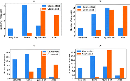
Note. (a) Q1, (b) Q2, (c) Q3, (d) Q4.

Note. (a) Q1, (b) Q2, (c) Q3, (d) Q4.
5.2. Alumni Surveys
A survey of course alumni was used to assess the impact of these courses beyond the classroom. Alumni surveys were sent after the most recent course iteration (fall 2020) to all students from both institutions who had completed the course (except for those from fall 2020 at the University of Toronto) and for whom we had active email addresses. In total, the survey was sent to 381 students from the University of Toronto and 66 students from the University of Wisconsin–Madison.
Table 3 provides descriptive characteristics about the 113 survey respondents from the University of Toronto and 42 respondents from the University of Wisconsin–Madison. The “Other” row for degree major included students from computer science, business, chemical engineering, and materials science engineering. For the University of Toronto students who indicated that they are working, the three most common industries were consulting, finance, and technology, with the most common job titles being analyst, consultant, and software engineer. For the University of Wisconsin–Madison, the three most common industries were technology, logistics, and healthcare and the most common job titles were analyst and software engineer. Students who listed “Other” for what they are doing now included internships and professional experience co-ops.
|
Table 3. Summary of Alumni Survey Data
| University of Toronto (n = 113) | University of Wisconsin–Madison (n = 42) | |
|---|---|---|
| When did you take the course? | ||
| Winter 2017 | 21 (18%) | — |
| Winter 2018 | 27 (24%) | — |
| Winter 2019 | 27 (24%) | — |
| Fall 2019 | 38 (34%) | 22 (52%) |
| Fall 2020 | — | 20 (48%) |
| What is/was your major? | ||
| Industrial engineering | 92 (81%) | 34 (81%) |
| Biomedical engineering | — | 2 (5%) |
| Civil engineering | — | 4 (10%) |
| Mechanical engineering | 2 (2%) | — |
| Engineering science | 16 (14%) | — |
| Other | 3 (3%) | 2 (5%) |
| When did you graduate? | ||
| 2017 | 10 (9%) | — |
| 2018 | 21 (19%) | — |
| 2019 | 24 (21%) | 4 (9%) |
| 2020 | 18 (16%) | 13 (31%) |
| Not yet | 40 (35%) | 25 (60%) |
| What are you doing now? | ||
| Working | 65 (58%) | 14 (33%) |
| Finishing my degree | 27 (24%) | 14 (33%) |
| Graduate school | 14 (12%) | 13 (31%) |
| Other | 7 (6%) | 1 (3%) |
In line with Section 5.1, we asked respondents to indicate how the course helped them develop skills related to each of four learning outcome questions (Q1 to Q4 above). Figure 3, (a) and (b) displays the results for each question for the University of Toronto and the University of Wisconsin-Madison, respectively. For both institutions, we observe a clear rightward skew in the distribution indicating that students believed they learned. For example, no student answered very little for any question across both institutions.
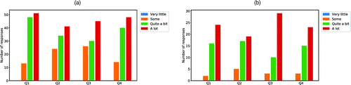
Note. (a) University of Toronto, (b) University of Wisconsin–Madison.
Next, we asked respondents three additional questions to assess how the course has impacted what they are doing now:
AQ1: To what extent are you using the skills learned from the course (including coding, data analysis, model development, problem solving, etc.)?
AQ2: To what extent have the skills learned from the course helped you succeed in other courses/your job/graduate school/other?
AQ3: To what extent has the course impacted your current/future career choice?
Figures 4 and 5 display the results for each of these questions stratified by the respondents current status for the University of Toronto and the University of Wisconsin-Madison, respectively. The results indicate that students are using the skills learned in these courses, regardless of what they are currently doing, and that the skills learned in the course have contributed to their success in current endeavors for most students. Finally, Figures 4(c) and 5(c) show that the course has had some impact on career choices, particularly for those students who are still finishing their degree. Some selected free form comments from the survey respondents are provided below that highlight how the course has been impactful beyond the classroom:
I really enjoyed the course. Together with my summer research experience it allowed to excel at my current position at Kijiji.
The final project was an amazing thing to work on and I have used it as examples of my work/learning during interviews.
Got a data science internship because of this course! Frequently referred to the labs on the job. Thanks!!
During my [co-op] I worked in a business strategy role, and the data science and analytics skills I learned from this course helped me design more creative and effective solution, and I was able to provide an analytical and data driven perspective in a pure business team. I think in the future I would explore more opportunities in business/data analytics!
This course was so impactful that I decided to switch my career very last minute because I was fascinated by the topics discussed in class. When I interviewed for my role at AWS, I used a project I completed in the class as the focal point in my interview presentation. I am in a generalist role at AWS right now, but I hope to specialize in AWS machine learning-related services in the future.
On almost all the project I have worked on at Grainger, I used something that I learned in this course.
The coding experience I got from the course has been very useful already, and I’ve seen a couple ways to use ML in related research in the future.

Note. (a) AQ1, (b) AQ2, (c) AQ3.
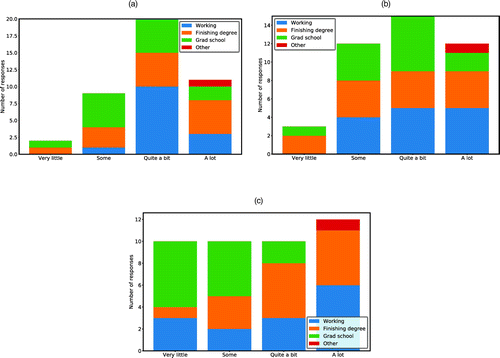
Note. (a) AQ1, (b) AQ2, (c) AQ3.
6. Student Course Evaluations
In this section, we present student course evaluations that highlight success toward addressing key course goals. Our institutions use an online system to solicit both quantitative and qualitative student evaluations on each course. We also present changes to the course that were driven by student feedback that we feel have significantly improved the course.
6.1. Quantitative Evaluations
We selected a subset of the course evaluation questions that are most directly related to the course objectives. For the University of Toronto course, we selected the following four questions:
A1: The course helped me improve my ability to formulate, analyze, and solve problems.
A2: The instructor related course concepts to practical applications and/or current research.
A3: I found the course intellectually stimulating.
A4: The course material inspired me to learn more about the subject matter.
For the University of Wisconsin–Madison course, we selected the following three questions:
B1: The instructor aroused my interest in the subject matter.
B2: The instructor related the course materials to real problems.
B3: The instructor stimulated my thinking.
Note that A2 is aligned with B2, A3 is aligned with B3, A4 is aligned with B1, and A1 does not have a match at the University of Wisconsin–Madison.
Table 4 displays the average numerical student evaluation scores for the University of Toronto course, compared with the department average, using a five-point scale with higher values corresponding to greater agreement. The exact mapping of numbers to responses is:1 (not at all), 2 (somewhat), 3 (moderately), 4 (mostly), and 5 (a great deal). The first three questions are included in the evaluation of all courses in the Faculty of Applied Science and Engineering. The last question, A4, is one from a large bank of questions that an instructor can select (up to three) each year to further personalize the course evaluation. Because these questions may not be widely used, there is no departmental average collected. Also, to diversify the evaluation data collected for this course, a different question was chosen in lieu of A4 in 2019. For questions A1, A2, and A3, we compute the average and standard deviation scores for the course (weighted by the number of responses) and the department (equal weighting because class sizes were unavailable). We assume that the annual class averages for each question are independently, identically, and normally distributed implying that standard hypothesis testing techniques can be used Montgomery (2007). The final two rows of Table 4 present the t-statistic and corresponding p-value of a hypothesis test with a null hypothesis that the observations from Analytics in Action and the department courses came from populations with the same mean (but unknown and potentially unequal variances).
|
Table 4. Student Evaluation Scores for the University of Toronto Course on a Five-Point Scale
| A1 | A2 | A3 | A4 | |||||||
|---|---|---|---|---|---|---|---|---|---|---|
| Year | Class size | Responses | Course | Dept. | Course | Dept. | Course | Dept. | Course | Dept. |
| 2017 | 102 | 44 | 4.4 | 3.6 | 4.8 | 4.0 | 4.4 | 3.8 | 4.7 | — |
| 2018 | 98 | 33 | 4.5 | 3.7 | 4.8 | 4.0 | 4.4 | 3.7 | 4.4 | — |
| 2019 | 90 | 41 | 4.5 | 3.7 | 4.9 | 3.8 | 4.4 | 3.7 | — | — |
| 2020 | 97 | 47 | 4.6 | 3.8 | 4.9 | 3.9 | 4.6 | 3.8 | 4.7 | — |
| Average | 4.50 | 3.70 | 4.85 | 3.93 | 4.46 | 3.75 | — | — | ||
| Std. dev. | 0.07 | 0.07 | 0.05 | 0.08 | 0.09 | 0.05 | — | — | ||
| t-stat | 16.16 | 19.5 | 13.79 | — | — | |||||
| p-value | 0.00 | 0.00 | 0.00 | — | — | |||||
Note. Std. dev., standard deviation; Dept., department.
Table 5 displays the average numerical student evaluation scores for the University of Wisconsin–Madison course (and the department average) using a four-point scale with the following mappings: 1 (strongly disagree), 2 (disagree moderately), 3 (agree moderately), and 4 (strongly Agree). Because only one year of data are available, we were unable to compute p-values.
|
Table 5. Student Evaluation Scores for the University of Wisconsin–Madison Course on a Four-Point Scale
| B1 | B2 | B3 | ||||||
|---|---|---|---|---|---|---|---|---|
| Year | Class size | Responses | Course | Dept. | Course | Dept. | Course | Dept. |
| 2020 | 33 | 22 | 4.0 | 3.6 | 4.0 | 3.6 | 4.0 | 3.3 |
Note. Dept., department.
Across the board, course evaluation scores were high, even with respect to departmental averages. Overall, the scores suggest that students developed a strong interest in the course material; improved their (self-perceived) analytics problem solving ability; and clearly saw the connection between this course and real, practical problems. However, it is important to acknowledge the limitations associated with student evaluation of teaching, which can be biased based on a range of factors (Basow 1995, Wachtel 1998). Future course iterations with more purposeful data collection will allow for additional evaluations.
6.2. Qualitative Evaluations
To supplement the numerical data presented above, we also present student comments submitted through the online evaluation system, with a focus on feedback that is related to our course goals and learning objectives. We present student comments in two main groups. First, both courses received encouraging evaluations to suggest we successfully built interest and excitement in machine learning:
The instructor sparked my interest in ML.
I found the lectures very interesting and inspiring, and I will highly recommend this course to students who have the opportunity to take it during their undergrad.
I feel like I really learned a lot in this course and that I will apply the skills learned. This course is the most useful course I have ever taken in university. I am using the skills learned in this course in both my thesis and my capstone! This is probably the best engineering course I have taken in my undergrad.
One of the best courses I’ve ever had; I gained valuable skills in ML and data processing.
Second, we received a plethora of positive feedback that suggests highlighting successful and innovative real-world applications of analytics, and using those applications to teach various technical methods was well received:
All the lectures were very interesting. Using real-life examples to teach us each method of using analytics (as the name of the course suggests in action) made every lecture much more interesting and relatable.
The lectures were very well planned out with engaging material. It was so cool to see applications from such a variety of fields (I didn’t expect law to be an application area!)—to see the real-world applications was very encouraging to me, as I expect to continue studying data analytics in grad school and build on the things we learnt here.
Probably the best course I have taken at University of Toronto so far! I loved the structure of the lectures and being able to learn about applications of analytics in such a variety of fields throughout the semester.
Presenting the course materials as case studies was excellent. I wished all courses did the same thing.
I appreciated all the relevant applications that the instructor used to introduce each of the algorithms that we learned.
I really appreciate the connections from theories and coding to the real-life cases! This way of learning definitely motivated me to learn more from the machine learning and OR field!
Overall, we have not received any resistance to teaching this material to an IEOR audience. Most of our students tend to be application driven and appreciate the use of concrete applications to teach the techniques. In fact, our main surprise is that our students generally have limited exposure to ML topics; these courses are often the first time students have been exposed to these techniques. For many students, these courses spark an interest to further develop these skills.
6.3. Changes Motivated by Student Evaluations
As part of the continual improvement process, we review student evaluations each year to identify opportunities to improve the learning experience. The following are changes that we have instituted based on those evaluations:
Switching to Python: The University of Toronto course was originally developed in Matlab to align with the “software spine” that runs throughout the curriculum. As other courses and general student interest shifted to Python, we modified the course accordingly, with students coding in Jupyter notebooks. As part of this change, we also introduced an introductory Python laboratory. Although students had encountered Python in a previous course, it was more focused on basic coding skills like understanding “for” loops. Our introductory laboratory focused on other relevant packages and skills, including Numpy and Pandas for handling and visualizing data and preparing it for machine learning activities.
Switching to cloud environment: The year after switching to Python, we made the move to switch to Google Colaboratory, allowing students to code and run their programs on Google’s cloud servers. The primary motivation for this switch, suggested by students and a TA, was to facilitate student collaboration on the major coding tasks of the project.
Modifying contact hours structure; After hearing and observing that students would benefit from more hands-on time, an extra hour of laboratory and a new one-hour tutorial were added in 2020 at University of Toronto, replacing an hour of lecture each week.
Modifying the grading scheme: The University of Toronto course originally placed more weight on the laboratory quizzes. But students consistently felt that the amount of work required to deliver a strong project was much more than the relative weight it received. This led to the current weightings described above. Similarly, student feedback also led to a small reduction in the relative weight of the presentation.
Modifying the exam structure: The first iteration of the University of Wisconsin-Madison course included a cumulative final exam. Motivated by student feedback, the second iteration will partition the cumulative final exam into two exams (one midway through the course and one at the end of the semester). This structure should allow students to dive deeper into current content, limit recency bias, and decrease the weight of a major final exam.
In addition to evaluations and feedback from the students, we continue to make tweaks to the course based on any novel circumstances that year. For example, at the University of Toronto, a Fall Reading Week was instituted for the first time in 2020, shortening the semester by one week. That coincided with the move to fewer lecture hours and more laboratory/tutorial hours, which meant that guest lectures had to be cut. At the University of Wisconsin–Madison, as a result of the COVID pandemic, the final exam was replaced with a project along with peer review, where students used a rubric to evaluate five peer presentations.
7. Conclusion
This paper describes two courses that introduce machine learning concepts to undergraduate, predominantly IEOR students. Instead of taking a methods-first approach, these courses use real-world applications to motivate, introduce, and explore these machine learning techniques and highlight meaningful overlap with operations research. Significant hands-on coding experience is used to build student proficiency with the techniques. Student feedback indicates that these courses have greatly increased student interest in machine learning and appreciation of the real-world impact that analytics can have and helped students develop practical skills that they can apply. We believe that similar application-driven courses that connect machine learning and operations research would be valuable additions to undergraduate OR curricula broadly.
We gratefully acknowledge current and former teaching assistants who have contributed greatly to the design and smooth operation of the course: Aaron Babier, Kyle Booth, Craig Fernandes, Rafid Mahmood, Yusuf Shalaby, Ian Zhu, Haoran Zhu, and Ari Smith. We thank George Almaria, Shannon Osborne, and Oscar Del Rio for their help with the University of Toronto alumni survey. Finally, We thank Qin Liu for her helpful discussions on evaluating student learning.
Appendix A.

Note. See Table 2 for a breakdown that includes the time spent on each topic.
Appendix B.
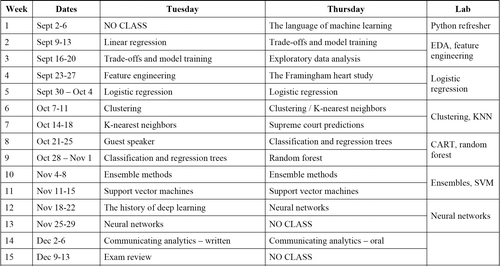
Note. See Table 2 for a breakdown that includes the time spent on each topic.
Appendix C.
The following subsections describe all course modules from our two courses (shown in Table 2); a single course does not include all of them. We provide the full list here for potential instructors to see what such a course might include. The University of Toronto course includes both predictive and prescriptive analytics methods (linear regression, logistic regression, clustering, CART/random forests, optimization, simulation, predict-then-optimize), whereas the University of Wisconsin–Madison course focuses exclusively on machine learning (linear regression, logistic regression, clustering, CART, ensembles, support vector machines (SVMs), deep learning).
C.1. Data Engineering
In data engineering, we focus on exploratory data analysis, data visualization, and feature creation. At the University of Toronto, these topics are not covered explicitly in lecture but are introduced in “Lab Zero” as part of an introduction to the Python environment and then reinforced through all subsequent labs. In that laboratory, we use a data set on chronic kidney disease (Dua and Graff 2017). Using this data set, students learn how to organize their data, combine data frames, impute missing data, and generate plots to visualize the data. The University of Wisconsin–Madison includes a lecture on data engineering that focuses on exploratory data analysis and feature engineering. A corresponding laboratory provides an opportunity for students to explore and clean a messy data set on medical supply chains.
C.2. Model Engineering
In model engineering, we focus on key concepts, such as the bias-variance trade-off; feature selection techniques; model training/testing strategies (e.g., cross validation, hyperparameter tuning); and commonly encountered problems, such as highly imbalanced classification data. Note that these concepts consistently appear in other modules as well. At the University of Toronto, model engineering is combined with the clustering module. In the laboratory, an application to predict loan repayment is used to explore concepts such as model selection, grid search, and model stacking. Because of the exclusive ML focus, the University of Wisconsin–Madison course includes a stand-alone module on model engineering that focuses on the concepts highlighted above, in addition to discussing the prediction-explanation trade-off. There is no specific model engineering laboratory at the University of Wisconsin–Madison because these concepts are reinforced through all labs and coding-based homework problems.
C.3. Linear Regression
This module reviews linear regression (typically students have seen it before in a previous statistics class) using two different applications presented in Bertsimas et al. (2016). The first application focuses on predicting the quality of wine and is inspired by a classic human versus machine debate that pits the linear regression models of Princeton Professor Orley Ashenfelter against the world’s foremost wine expert, Robert Parker (Passell 1990, Ashenfelter et al. 1995, Ashenfelter 2008). The application demonstrates that wine quality, with price as the target variable, can be predicted with a few simple variables on weather and temperature. The second application was inspired by the book Moneyball: The Art of Winning an Unfair Game, which chronicled the journey of the Oakland Athletics, a Major League Baseball team, in using analytics to gain a competitive edge (Lewis 2004). We demonstrate how a series of regression models can predict team wins based on individual player statistics.
The technical content focuses on the linear regression equation, modeling assumptions, transforming data, the ordinary least squares problem, and regularization. This module also provides an opportunity to discuss model evaluation metrics in general, which we specialize to the linear regression context by discussing mean squared error and R2.
The laboratory component provides students with real data from the application (e.g., either wine or Moneyball data) so that they can replicate the models, experiment with their own ideas, and answer follow-up/what-if questions, such as how many more runs does a team need to win an additional game and is more or less summer rain better for wine quality? The laboratory also gives students an opportunity to implement regularized linear regression models and see the effect on potentially overfit models.
C.4. Logistic Regression
In this module, we introduce classification problems using logistic regression. The main application we use to teach logistic regression was taken from Bertsimas et al. (2016) and focuses on the Framingham Heart Study, which was considered one of the top 10 cardiology advances of the 1900s by the Texas Heart Institute Journal (Mehta and Khan 2002). The Framingham Heart Study was commissioned by the U.S. Congress in 1948 and has been collecting data for over 70 years (Mahmood et al. 2014). Much of our current understanding of the risk factors that affect heart disease can be traced back to this study (e.g., discovering that smoking increases the risk of heart disease), and the Framingham data have contributed to over 3,000 scientific papers (Andersson et al. 2019).
The technical content focuses on the connection with linear regression (e.g., via the logit link function), how to interpret the regression coefficients, maximum likelihood estimation, and regularization. Similar to linear regression, this module provides an opportunity to discuss various metrics for evaluating classification models, such as confusion matrices, receiver operating curves, and the implications of the trade-off between false positives and false negatives.
In the laboratory component, students use a sample of the original Framingham data from the 1950s to build previously developed models (e.g., Framingham risk score) and to explore the relationships between various features (e.g., smoking, age, etc.) and heart disease.
C.5. Clustering/k-Nearest Neighbors
This module focuses on a combination of “spatial” techniques including hierarchical clustering, K-means clustering, and k-nearest neighbors. We have used two applications for this module. The first focuses on introducing students to text and sentiment analysis using news articles from past presidential elections. Each word is represented as a feature and the goal is to use clustering to determine the key topics/threads from the election cycle. A clustering laboratory based on sentiment analysis provides students with real data from the 2004 presidential election. The second application considers the problem of defining player types in hockey using individual performance data (Chan et al. 2012). Players are clustered based on their statistics to identify different types of forwards, defensemen, and goalies. Real-world motivations come from forming Olympic hockey teams—they tend not to be “balanced” in player types but overwhelmingly have offensively oriented forwards, for example—and identifying comparables for salary arbitration and future career projections. We also consider the problem of attributing team performance to different player types, which allows us to introduce the concept of using variables derived from clustering in a regression model.
The technical focus for this module is on the algorithmic structure of these methods (because they are quite simple) and on key practical considerations (e.g., the importance of data-scaling). We also use this module to highlight the differences/similarities between supervised and unsupervised learning (because clustering is the first and only unsupervised model in our courses).
C.6. Classification and Regression Trees
We introduce CART using two applications. The first was adapted from Bertsimas et al. (2016) and discusses the use of CART to forecast Supreme Court decisions (Martin et al. 2004, Ruger et al. 2004). CART models are trained and inspected for each Supreme Court justice as a means of trying to understand patterns in their decision making. The performance of the models is compared against a panel of experts (e.g., law professors, lawyers, clerks, etc.) in a human versus machine competition. The second is based on a tool, Patternizr, which was implemented by the New York Police Department to identify crime patterns, defined as a series of individual crimes committed by the same person (Chohlas-Wood and Levine 2019). In addition to showcasing the power of CART, this case enables rich discussions on ethics and real-world implementation of machine learning tools.
The technical content focuses primarily on the original CART algorithm developed by Breiman et al. (1984), how a CART tree can be used for both interpretation and prediction, and how optimization models can be used to design optimal CART trees (Bertsimas and Dunn 2017).
The laboratory component investigates vandalism in Wikipedia, which is specifically referred to as pages that have had information removed, incorrect information added, or the presence of inappropriate content. Students use a data set that summarizes the revision history for the “Language” entry on Wikipedia (en.wikipedia.org/wiki/Language) and attempt to predict whether a particular revision was an instance of vandalism or not.
C.7. Ensemble Methods
This module focuses on ensemble methods, including boosting, bagging, and stacking. We use two applications. The first highlights the $1,000,000 Netflix Prize Competition, which ran from 2006–2009 and was ultimately won by an ensemble model (Lakhani et al. 2014, Amatriain and Basilico 2015). In fact, the winning team was actually an ensemble of teams, where each team used an ensemble model. This application allows us to highlight methodological breakthroughs that contributed to the success of ensembles throughout the competition, such as simultaneously training each “learner” and the idea of blended stacking.
The second application is used in the laboratory and based on research that uses random forest models to predict travel times in developing urban centers (Boutilier and Chan 2020). Students are provided with real travel time data from Dhaka, Bangladesh and are asked to compare various ensemble algorithms, such as AdaBoost and random forest.
The technical component of this module focuses on building intuition for when to use bagging vs. boosting in connection with the bias-variance trade-off and on the algorithmic structure of the models. We focus specifically on the Adaboost algorithm for boosting and the random forest algorithm for bagging.
C.8. Support Vector Machines
For IEOR students, support vector machines are an excellent topic because they are formulated and solved as a convex optimization problem (specifically a quadratic program). In this module, we use the ImageNet competition as our primary application (Deng et al. 2009). ImageNet was an image classification competition that included more than 14 million hand-annotated images, and SVMs achieved the highest accuracy for the first few years of the competition. In addition to showcasing the power of SVMs, this example is used to demonstrate the value associated with large-scale machine learning competitions. The competition led to several breakthroughs (including the use of graphics processing units to train neural networks); the 2012 ImageNet competition was a key turning point in machine learning history, when a neural network first won the competition (by a staggering 10%). Hence, this application can also serve as an excellent lead-in to the deep learning module.
As noted above, the technical content of SVMs is highly relevant for IEOR students. We focus primarily on the quadratic programming formulation and on why the dual formulation is typically solved in practice (because of computational benefits and improved structure). We also use this module to demonstrate the connection between optimization and machine learning and showcase how optimization can be used to train machine learning models.
C.9. Deep Learning
The lecture module on deep learning and neural networks does not follow the typical application-based format. Instead, we tell a chronological story about the history of deep learning because the story itself has useful insights, including the long history of neural network research (this is not a new field!) and the importance of key breakthroughs (e.g., multilayer perceptrons and back propagation). Throughout the story, we highlight important applications and use-cases, including LeNet (a digit recognition network used by banks for remote check deposits) (LeCun et al. 1990, Le Cun et al. 1997), self-driving cars (Bojarski et al. 2016, Maqueda et al. 2018), and personalized medicine (e.g., diabetic retinopathy detection) (Gulshan et al. 2016, Norgeot et al. 2019). We also use the story to teach various technical topics as they appear, including the original perceptron, multilayer perceptrons, back propagation, and the different types of neural networks. The lecture concludes with a deep dive into using deep learning and AI to play games, such as Go, Chess, and Shogi, based on Google’s AlphaGo (Silver et al. 2016, 2017, 2018). Instead of a traditional laboratory, we use this module as an opportunity to conduct an in-class ethics discussion on the use and future of AI, with a focus on personalized medicine and self-driving cars.
C.10. Linear Optimization
Because linear optimization is a technique that all students in the course are familiar with, this module covers some advanced topics in linear optimization, using radiation therapy for cancer as the motivating application. The first application involves the design of robust treatments, those that are desensitized to uncertainties like organ motion (Chan et al. 2006, Bortfeld et al. 2008), using a robust linear optimization model. Then, we demonstrate that adapting a treatment from day to day, while accounting for intratreatment uncertainty using robust optimization, can further improve the quality of treatments. Overall, this case conveys to students the crucial role that optimization plays in the planning of life-saving treatments. The second case uses radiation therapy to illustrate the concept of inverse optimization (Ahuja and Orlin 2001). In particular, we demonstrate that key parameters in the treatment optimization model can be “learned” from historical treatments (Chan et al. 2014).
We then demonstrate that inverse optimization can be effective in a predict-then-optimize pipeline for creating new treatments in an automated fashion: (1) a neural network model is used to predict clinically acceptable and patient-specific dose distributions, (2) inverse optimization is used to learn parameters from this dose, (3) and then these parameters are used in an optimization model to design the final treatment (reference blinded). In step (2), the predicted dose from step (1) is considered a feasible solution to the treatment optimization problem and inverse optimization is used to derive objective function parameters that produce a treatment with dosimetric properties as close as possible to the predicted dose. In this application, machine learning and inverse optimization are used synergistically to generate personalized doses and derive model parameters to recreate these doses, respectively (Babier et al. 2019).
In the laboratory, we provide students with radiation therapy data and allow them to experiment with different objective functions to fine-tune the resulting treatment. The trial-and-error process of tuning the objective function and inspecting the resulting treatment mimics the current clinical workflow that automated planning methods are in the process of disrupting.
C.11. Integer Optimization
Two applications are used to illustrate integer optimization. The first focuses on the placement of public access defibrillators to enable bystander response to cardiac arrest. After motivating the importance of rapid response and defibrillator access, we discuss how coverage-based models can be used to identify optimal locations from a discrete set considering spatiotemporal availability and model realistic bystander retrieval scenarios, compared with the current practice on placement (Chan et al. 2013, 2016; Sun et al. 2016, 2019). We then introduce the concept of drone-delivered defibrillators—a topic that is currently being tested in multiple jurisdictions around the world—and demonstrate how a drone network can be designed using integer optimization and queuing (Boutilier et al. 2017). The second application describes the construction of a new building for (hospital name blinded) in (city name blinded) and the need to redesign their ambulatory clinic schedule using integer optimization to meet the space requirements of the new building (Eagen et al. 2018).
Although neither topic focuses on machine learning explicitly, they do provide a nice opportunity to discuss real-world integer optimization applications and set up the class for the predict-then-optimize module. For example, in the context of defibrillator placement, we discuss the stability of spatiotemporal patterns of cardiac arrest and whether they are predictable, which can then inform location decisions.
The laboratory for this module reinforces integer optimization modeling techniques that students would have seen in a previous OR course but in Python, which they have not used in the previous optimization course. This prepares the students for subsequent implementations combining machine learning and optimization in Python. We use chess as the motivating application: students form the ultimate chess team for a tournament by solving a knapsack problem with side constraints. This application continues into the simulation laboratory, which considers prediction and Monte Carlo simulation.
C.12. Simulation
The simulation module considers two applications. The first uses blackjack to illustrate Monte Carlo simulation, using a lecture developed by Bertsimas et al. (2016). Going back to the roots of blackjack analysis and card counting (Thorp 1966), we demonstrate how simulation can be used to determine the “value” of a particular card (i.e., whether a card increases or decreases a player’s chance of winning a single hand) by simulating thousands of games with that card removed from the deck. The second application uses the classic Markov chain model of a tennis match to demonstrate how simulation can be used to estimate match winning probabilities (Riddle 1988). We then use the Markov chain as a launching-off point to describe a Markov decision process model for tennis handicapping (Chan and Singal 2016) and the use of simulation to compare the performance of the optimal policy versus intuitive heuristics.
In the laboratory, we combine prediction and simulation concepts in the aforementioned chess application. Once the team is formed via optimization, the goal is to simulate a chess tournament using Monte Carlo simulation. To predict the outcome (win/loss/draw) of a given match, students build a multinominal logistic regression model using the ELO rating of the two players.
C.13. Predict-then-Optimize
The module on predict-then-optimize comprises several applications that combine machine learning and optimization. One application is motivated by the matching process of eHarmony, taken from Bertsimas et al. (2016). Logistic regression is used to estimate the probability that two users will communicate (their “affinity score”) when a match is suggested by the platform. These probabilities then become objective function parameters in a transportation problem that decides which users to match to others to maximize the total or average affinity score, given certain matching constraints.
Another application combines machine learning with optimization to aid refugee resettlement (Ahani et al. 2021). Logistic regression and gradient boosted regression trees predict the probability of refugee employment in different locations, and then an integer optimization model optimizes the assignment of refugee families to different communities to maximize total expected employment. The logistic regression includes a lasso constraint, providing an opportunity to reinforce regularization as a method for addressing overfitting.
A final application studies the value of positional flexibility in baseball—that is, how many wins a player who can play multiple positions is worth over a player who can only play a single position—integrating prediction, simulation, and optimization (Chan and Fearing 2019). Regression models are used to estimate the ability of players playing different positions and the probability/length of injury during a season. Simulation is used to draw from the injury distributions, and then optimization is used to quantify the performance of the roster given the estimated player capabilities and simulated injury durations.
This module integrates several previous modules and demonstrates to students how to solve problems requiring a combination of different analytics methodologies.
C.14. Communicating Analytics
We developed a lecture on “communicating analytics” that provides concrete suggestions on how to present analytics work in both written and oral formats. For written communication, we discuss the importance of outlines, structuring text that is particularly heavy in technical detail, balancing the amount of detail that is presented in the main methodology section with the appendix, and ensuring broader takeaways are clearly communicated. As an example, we show several side-by-side images of two passages of text, representing “before” and “after” editing. The goal is to provide concrete examples of how to “trim the fat” and effectively structure technical writing. We also highlight how the various sections change depending on the audience (e.g., writing for a medical audience versus an operations research audience). For oral communication, we discuss the importance of an organized presentation and visual slides, how to prepare for a research presentation, and tips from our personal experiences. Because of major changes in the course structure at the University of Toronto in fall 2020, this lecture was not given. We aim to integrate this lecture back into the course in the future.
References
- , (2021) Placement optimization in refugee resettlement. Oper. Res., ePub ahead of print March 24, https://doi.org/10.1287/opre.2020.2093.Link, Google Scholar
- (2001) Inverse optimization. Oper. Res. 49(5):771–783.Link, Google Scholar
- (2015) Recommender systems in industry: A Netflix case study. Ricci F, Rokach L, Shapira B, Kantor PB, eds. Recommender Systems Handbook (Springer, New York), 385–419.Crossref, Google Scholar
- (2019) 70-year legacy of the Framingham Heart Study. Nature Rev. Cardiology 16(11):687–698.Crossref, Google Scholar
- (2008) Predicting the quality and prices of Bordeaux wine. Econom. J. (London) 118(529):F174–F184. Crossref, Google Scholar
- (1995) Bordeaux wine vintage quality and the weather. Chance 8(4):7–14.Crossref, Google Scholar
- (2019) Knowledge-based automated planning with three-dimensional generative adversarial networks. Medical Physics 47(2):297–306. Crossref, Google Scholar
- (1995) Student evaluations of college professors: When gender matters. J. Ed. Psych. 87(4):656.Crossref, Google Scholar
- (2006) The interplay of optimization and machine learning research. J. Machine Learn. Res. 7(Jul):1265–1281.Google Scholar
- (2013) Validity of student self-reported ratings of learning. Assessment Evaluation Higher Ed. 38(4):377–388.Crossref, Google Scholar
- (1996) Neuro-Dynamic Programming (Athena Scientific, Nashua, NH).Google Scholar
- (2017) Optimal classification trees. Machine Learn. 106(7):1039–1082.Crossref, Google Scholar
- (2016) The Analytics Edge (Dynamic Ideas LLC, Charlestown, MA).Google Scholar
- (2006) Pattern Recognition and Machine Learning (Springer, New York).Google Scholar
- (2016) End to end learning for self-driving cars. Preprint, submitted April 25, https://arxiv.org/abs/1604.07316.Google Scholar
- (2008) Robust management of motion uncertainty in intensity-modulated radiation therapy. Oper. Res. 56(6):1461–1473.Link, Google Scholar
- (2020) Ambulance emergency response optimization in developing countries. Oper. Res. 68(5):1315–1334.Link, Google Scholar
- (2017) Optimizing a drone network to deliver automated external defibrillators. Circulation 135(25):2454–2465.Crossref, Google Scholar
- (2004) Convex Optimization (Cambridge University Press, Cambridge, UK).Crossref, Google Scholar
- (1984) Classification and Regression Trees (Chapman & Hall/CRC, Boca Raton, FL). [Database]Google Scholar
- (2019) Process flexibility in baseball: The value of positional flexibility. Management Sci. 65(4):1642–1666. Link, Google Scholar
- (2016) A Markov decision process-based handicap system for tennis. J. Quant. Anal. Sports 12(4):179–188.Google Scholar
- (2006) A robust approach to IMRT optimization. Physics Medicine Biol. 51(10):2567–2583.Crossref, Google Scholar
- (2012) Quantifying the contribution of NHL player types to team performance. Interfaces 42(2):131–145. Link, Google Scholar
- (2016) Optimizing the deployment of public access defibrillators. Management Sci. 62(12):3617–3635.Link, Google Scholar
- (2014) Generalized inverse multiobjective optimization with application to cancer therapy. Oper. Res. 62(3):680–695.Link, Google Scholar
- (2013) Identifying locations for public access defibrillators using mathematical optimization. Circulation 127(17):1801–1809.Crossref, Google Scholar
- (2019) A recommendation engine to aid in identifying crime patterns. INFORMS J. Appl. Analytics 49(2):154–166.Link, Google Scholar
- (1993) Neural Networks for Optimization and Signal Processing (John Wiley & Sons, Inc., New York).Google Scholar
- (2020) Roundup of machine learning forecasts and market estimates. Forbes (January 19), https://www.forbes.com/sites/louiscolumbus/2020/01/19/roundup-of-machine-learning-forecasts-and-market-estimates-2020/#45b3d5a75c02.Google Scholar
- (2009)
Imagenet: A large-scale hierarchical image database . 2009 IEEE Conf. Comput. Vision Pattern Recognition (IEEE, Piscataway, NJ), 248–255.Crossref, Google Scholar - (2017) UCI machine learning repository. Accessed April 1, 2021 http://archive.ics.uci.edu/ml.Google Scholar
- (2018) Women’s college hospital uses operations research to create an ambulatory clinic schedule. Service Sci. 10(3):230–240. Link, Google Scholar
- (2001)
Graphviz—Open source graph drawing tools . Mutzel P, Junger M, Leipert S, eds. Graph Drawing, Lecture Notes in Computer Science, vol. 2265 (Springer, Berlin, Heidelberg), 483–484.Google Scholar - (2017) Smart “predict, then optimize.” Preprint, submitted October 22, https://arxiv.org/abs/1710.08005.Google Scholar
- (2019) Machine learning education for artists, musicians, and other creative practitioners. ACM Trans. Comput. Ed. 19(4):1–32 (TOCE). Crossref, Google Scholar
- (2016) Development and validation of a deep learning algorithm for detection of diabetic retinopathy in retinal fundus photographs. JAMA 316(22):2402–2410. Crossref, Google Scholar
- (2020) Array programming with NumPy. Nature 585:357–362.Crossref, Google Scholar
- (2009) Online Stochastic Combinatorial Optimization (The MIT Press, Cambridge, MA).Google Scholar
- (2007) Matplotlib: A 2d graphics environment. Comput. Sci. Engrg. 9(3):90–95.Crossref, Google Scholar
- (2014) Netflix: Designing the Netflix Prize. Harvard Business School Case (615-015).https://www.hbs.edu/faculty/Pages/item.aspx?num=47650#:˜:text=Netflix%3A%20Designing%20the%20Netflix%20Prize%20(A),-By%3A%20Karim%20R&text=Hastings%20determined%20that%20a%2010,by%20up%20to%20%2489%20million.Google Scholar
- (2010) Learning machine learning: A case study. IEEE Trans. Ed. 53(4):672–676.Crossref, Google Scholar
- (1997) Reading checks with multilayer graph transformer networks. 1997 IEEE Internat. Conf. Acoustics, Speech, Signal Processing, vol. 1 (IEEE, Piscataway, NJ), 151–154.Crossref, Google Scholar
- (1990)
Handwritten digit recognition with a back-propagation network. Touretzky DS, ed . Advances in Neural Information Processing Systems 2 (Morgan Kaufmann Publishers Inc., San Francisco), 396–404.Google Scholar - (2004) Moneyball: The Art of Winning an Unfair Game (WW Norton & Company, New York).Google Scholar
- (2014) The Framingham Heart Study and the epidemiology of cardiovascular disease: A historical perspective. Lancet 383(9921):999–1008. Crossref, Google Scholar
- (2018)
Event-based vision meets deep learning on steering prediction for self-driving cars . Proc. IEEE Conf. Comput. Vision Pattern Recognition (IEEE, Piscataway, NJ), 5419–5427.Crossref, Google Scholar - (2004) Competing approaches to predicting supreme court decision making. Perspect. Politics 2(4):761–767.Crossref, Google Scholar
- (2010) Data structures for statistical computing in Python. van der Walt S, Millman J, eds. Proc. 9th Python Sci. Conf. (Austin, TX), 56–61. Google Scholar
- (2002) Cardiology’s 10 greatest discoveries of the 20th century. Texas Heart Inst. J. 29(3):164.Google Scholar
- (2020) Equalizing Data Science Curriculum for Computer Science Pupils (Association for Computing Machinery, New York). Crossref, Google Scholar
- (2020) Data analytics in operations management: A review. Manufacturing Service Oper. Management 22(1):158–169.Link, Google Scholar
- (2007) Introduction to Statistical Quality Control (John Wiley & Sons, New York).Google Scholar
- (2019) A call for deep-learning healthcare. Nature Medicine 25(1):14–15.Crossref, Google Scholar
- (1990) Wine equation puts some noses out of joint. New York Times (March 4), https://www.nytimes.com./1990/03/04/us/wine-equation-puts-some-noses-out-of-joint.html.Google Scholar
- (2011) Scikit-learn: Machine learning in Python. J. Machine Learn. Res. 12:2825–2830. [Database]Google Scholar
- (1988) Probability models for tennis scoring systems. J. Roy. Statist. Soc. Ser. C. Appl. Statist. 37(1):63–75. Google Scholar
- (2004) The supreme court forecasting project: Legal and political science approaches to predicting supreme court decision making. Columbia Law Rev. 104:1150–1210. Crossref, Google Scholar
- (2015) Deep learning in neural networks: An overview. Neural Networks 61:85–117. Crossref, Google Scholar
- (2016) Mastering the game of go with deep neural networks and tree search. Nature 529(7587):484.Crossref, Google Scholar
- (2018) A general reinforcement learning algorithm that masters chess, shogi, and go through self-play. Science 362(6419):1140–1144. Crossref, Google Scholar
- (2017) Mastering the game of go without human knowledge. Nature 550(7676):354–359.Crossref, Google Scholar
- (1999) Neural networks for combinatorial optimization: A review of more than a decade of research. INFORMS J. Comput. 11(1):15–34. Link, Google Scholar
- (2019) What is hard about teaching machine learning to non-majors? Insights from classifying instructors’ learning goals. ACM Trans. Comput. Ed. 19(4):1–16 (TOCE). Crossref, Google Scholar
- (2016) Overcoming spatial and temporal barriers to public access defibrillators via optimization. J. Amer. College Cardiology 68(8):836–845.Crossref, Google Scholar
- (2019) In silico trial of optimized vs. actual public defibrillator locations. J. Amer. College Cardiology 74(12):1557–1567.Crossref, Google Scholar
- (1999) Between mdps and semi-mdps: A framework for temporal abstraction in reinforcement learning. Artificial Intelligence 112(1-2):181–211. Crossref, Google Scholar
- (1966) Beat the Dealer: A Winning Strategy for the Game of Twenty One, vol. 310 (Vintage Books, New York).Google Scholar
- (2020) SciPy 1.0: Fundamental algorithms for scientific computing in Python. Nature Methods 17:261–272.Crossref, Google Scholar
- (1998) Student evaluation of college teaching effectiveness: A brief review. Assessment Evaluation Higher Ed. 23(2):191–212.Crossref, Google Scholar
- (2020) mwaskom/seaborn v0.11.0. http://dx.doi.org/10.5281/zenodo.592845.Google Scholar
- (2017) Machine learning modules for all disciplines. Proc. 2017 ACM Conf. Innovation Tech. Comput. Sci. Ed. (ACM, New York), 84–85. Google Scholar