Efficient Scenario Generation for Heavy-Tailed Chance Constrained Optimization
Abstract
We consider a generic class of chance-constrained optimization problems with heavy-tailed (i.e., power-law type) risk factors. As the most popular generic method for solving chance constrained optimization, the scenario approach generates sampled optimization problem as a precise approximation with provable reliability, but the computational complexity becomes intractable when the risk tolerance parameter is small. To reduce the complexity, we sample the risk factors from a conditional distribution given that the risk factors are in an analytically tractable event that encompasses all the plausible events of constraints violation. Our approximation is proven to have optimal value within a constant factor to the optimal value of the original chance constraint problem with high probability, uniformly in the risk tolerance parameter. To the best of our knowledge, our result is the first uniform performance guarantee of this type. We additionally demonstrate the efficiency of our algorithm in the context of solvency in portfolio optimization and insurance networks.
Funding: The research of B. Zwart is supported by the NWO (Dutch Research Council) [Grant 639.033.413]. The research of J. Blanchet is supported by the Air Force Office of Scientific Research [Award FA9550-20-1-0397], the National Science Foundation [Grants 1820942, 1838576, 1915967, and 2118199], Defense Advanced Research Projects Agency [Award N660011824028], and China Merchants Bank.
1. Introduction
In this paper, we consider the following family of chance constrained optimization problems:
Chance constrained optimization problems have a rich history in operations research. Introduced by Charnes et al. (1958), chance constrained optimization formulations have proved to be versatile in modeling and decision making in a wide range of settings. For example, Prekopa (1970) used these types of formulations in the context of production planning. The work of Bonami and Lejeune (2009) illustrates how to take advantage of chance constrained optimization formulations in the context of portfolio selection. In the context of power and energy control the use of chance constrained optimization is illustrated in Andrieu et al. (2010). These are just examples of the wide range of applications that have benefited (and continue to benefit) from chance constrained optimization formulations and tools.
Consequently, there has been a significant amount of research effort devoted to the solution of chance constrained optimization problems. Unfortunately, however, these types of problems are provably NP-hard in the worst case (Luedtke et al. 2010). As a consequence, much of the methodological effort has been placed into developing (a) solutions in the case of specific models; (b) convex and, more generally, tractable relaxations; (c) combinatorial optimization tools; and (d) Monte Carlo sampling schemes. Of course, hybrid approaches are also developed. For example, as a combination of type b and type d approaches, Hong et al. (2011) show that the solution to a chance constraint optimization problem can be approximated by optimization problems with constraints represented as the difference of two convex functions. In turn, this is further approximated by solving a sequence of convex optimization problems, each of which can be solved by a gradient based Monte Carlo method. Another example is Peña-Ordieres et al. (2020), which combines relaxations of type b with sample-average approximation associated with type d methods. In addition to the aforementioned types, Hong et al. (2021) provides an upper bound for the chance constraint optimization problem using a robust optimization with a data-driven uncertainty set, achieving a dimension independent sample complexity.
Examples of type a approaches include the study of Gaussian or elliptical distributions when ϕ is affine both in L and x. In this case, the problem admits a conic programming formulation, which can be efficiently solved (Lagoa et al. 2005). Type b approaches include Hillier (1967); Seppälä (1971); Ben-Tal and Nemirovski (2000, 2002); Prékopa (2003); Bertsimas and Sim (2004); Nemirovski and Shapiro (2006a); Chen et al. (2010); and Tong et al. (2022). These approaches usually integrate probabilistic inequalities such as Chebyshev’s bound, Bonferroni’s bound, Bernstein’s approximations, or large deviation principles to construct tractable analytical approximations. Type c methods are based on branch and bounding algorithms, which connect squarely with the class of tools studied in areas such as integer programming (Ahmed and Shapiro 2008, Luedtke et al. 2010, Küçükyavuz 2012, Luedtke 2014, Zhang et al. 2014, Lejeune and Margot 2016). Type d methods include the sample gradient method, the sample average approximation, and the scenario approach. The sample gradient method is usually combined with a smooth approximation (see Hong et al. (2011) for example). The sample average approximations studied by Luedtke and Ahmed (2008) and Barrera et al. (2016), although simplifying the constraint’s probabilistic structure via replacing the population distribution by sampled empirical distribution, are nevertheless hard to solve due to nonconvex feasible regions. The method we consider in this paper is the scenario approach. The scenario approach is introduced and studied in Calafiore and Campi (2005) and is further developed in a series of papers, including Calafiore and Campi (2006); Nemirovski and Shapiro (2006b).
The scenario approach is the most popular generic method for (approximately) solving chance constrained optimization. The idea is to sample a number N of scenarios (each scenario consists of a sample of L) and enforce the constraint in all of these scenarios. The intuition is that if for any scenario, say , the constraint is convex in x, and is small, we expect that by suitably choosing N the constrained regions can be relaxed by enforcing for all , leading to a good and, in some sense, tractable (if N is of moderate size) approximation of the chance constrained region. Of course, this intuition is correct only when is small and we expect the choice of N to be largely influenced by this asymptotic regime.
By choosing N sufficiently large, the scenario approach allows obtaining both upper and lower bounds which become asymptotically tighter as . In a celebrated paper, Calafiore and Campi (2006) provide rigorous support for this claim. In particular, given a confidence level , if , with probability at least , the optimal solution of the scenario approach relaxation is feasible for the original chance constrained problem and, therefore, an upper bound to the problem is obtained. Unfortunately, the required sample size of N grows with as δ becomes small, limiting the scope of the scenario methods in applications.
Many applications of chance constraint optimization require a very small δ. For example, in the 5G ultra-reliable communication system design, the failure probability δ is no larger than (Alsenwi et al. 2019); for fixed income portfolio optimization, an investment grade portfolio has a historical default rate of , reported by Frank (2008).
Motivated by this, Nemirovski and Shapiro (2006b) developed a method that lowers the required sample size to the order of , making additional assumptions on the function (which is taken to be biaffine), and the risk factors L, which are to be assumed light-tailed. Specifically, the moment generating function is assumed to be finite in a neighborhood of the origin. No guarantee is given in terms of how far the upper bound is from the optimal value function of the problem as .
In the present paper, we focus on improving the scalability of N in terms of for the practically important case of heavy-tailed risk factors. Heavy-tailed distributions appear in a wide range of applications in science, engineering, and business (Wierman and Zwart 2012, Embrechts et al. 2013) but, in some aspects, are not as well understood as light-tails. One reason is that techniques from convex duality cannot be applied as the moment generating function of L does not exist in a neighborhood of zero. In addition, probabilistic inequalities, exploited in Nemirovski and Shapiro (2006b), do not hold in this setting. Only very recently, a versatile algorithm for heavy-tailed rare event simulation has been developed in Chen et al. (2019).
The main contribution of our paper is to develop an algorithm that has a sample complexity N uniformly bounded in the risk tolerance parameter, assuming a versatile class of heavy-tailed distributions for L. Specifically, we shall assume that L follows a semiparametric class of models known as multivariate regular variation, which is quite standard in multivariate heavy-tail modeling (Embrechts et al. 2013, Resnick 2013). Moreover, our estimator is shown to be within a constant factor to the solution to () with high probability, uniformly as . We are not aware of other approaches that provide a uniform performance guarantee of this type.
The main idea of our algorithm is to construct an analytically tractable event that uniformly contains the violation events for all x plausible to be feasible. In view of the reformulation of the probabilistic constraint in () as , the problem () can be solved by the scenario approach where L is sampled from the conditional distribution given . The risk tolerance parameter is adjusted to . The primary challenge is to construct as tight as possible so that the new risk tolerance parameter is bounded. (This is at the heart of Property 1 defined later. This property is facilitated in the heavy-tailed setting if we assume that has appropriate scaling properties, similar to the distribution of L uniformly over a suitable compact set of decisions.)
We illustrate our assumptions and our framework with a risk problem of independent interest. This problem consists in computing a collective salvage fund in a network of financial entities whose liabilities and payments are settled in an optimal way using the Eisenberg-Noe model (Eisenberg and Noe 2001). The salvage fund is computed to minimize its size to guarantee a probability of collective default after settlements of less than a small prescribed margin. For the sake of demonstrating the broad applicability of our method, we also present a portfolio optimization problem with value-at-risk constraints as an additional running example.
The rest of the paper is organized as follows. In Section 2, we introduce the portfolio optimization problem and the minimal salvage fund problem as particular applications of chance constraint optimization. We use both problems as running examples to provide a concrete and intuitive explanation for the concepts we introduce throughout the paper. In Section 3, we provide a brief review of the scenario approach in Calafiore and Campi (2006). The ideas behind our main algorithmic contributions are given in Section 4, where we introduce its intuition, rooted in ideas originating from rare event simulation. Our algorithm requires the construction of several auxiliary functions and sets, and we summarized the explicit expressions of the sets for the running examples in Table 1. How to do this for a more general setting is detailed in Section 5, in which we also present several additional technical assumptions required by our constructions. In Section 5, we also explain that our procedure results in an estimate that is within a constant factor of the optimal solution of the underlying chance constrained problem with high probability as . In Section 6, we show that the assumptions imposed are valid in our motivating example (as well as a second example with quadratic cost structure inside the probabilistic constraint). Numerical results for the examples are provided in Section 7. Throughout our discussion, in each section we present a series of results that summarize the main ideas of our constructions.
|

Table 1. Examples of and That Satisfy Property 1 When L Is Multivariate Regularly Varying
| Examples | Outer approximation set | Uniform conditional event |
|---|---|---|
| Portfolio optimization (1) | ||
| Minimal salvage fund (3) |
To keep the discussion fluid, we present the corresponding proofs in Appendix A unless otherwise indicated. In Appendix B, we introduce an importance sampling algorithm to sample from a parametric family of regularly varying distribution. We present additional numerical experiments in Appendix C.
1.1. Notations
In the rest of this paper, is the set of nonnegative real numbers, is the set of positive real numbers, and is the extended real line. A column vector with zeros is denoted by , and a column vector with ones is denoted by . For any matrix Q, the transpose of Q is denoted by ; the Frobenius norm of Q is denoted by . The identity matrix is denoted by I. For and , we use to denote the scalar multiplication of x with α. For two column vectors , we say if and only if . For a column vector and a scalar , we say that if and only if . For and , we define . The optimal value of an optimization problem is denoted by . For any real-valued random variable X with probability measure , define the inverse tail distribution function as . We also use Landau’s notation. In particular, if and are nonnegative real valued functions, we write if for some and if for some .
2. Running Examples
2.1. Portfolio Optimization with Value-at-Risk Constraint
We first introduce a portfolio optimization problem. Suppose that there are d assets to invest. If we invest a dollar in the jth asset, the investment has mean return μj and a nonnegative random loss Lj. Let represent the amount of dollars invested in different assets, and let and . We assume that L follows a multivariate heavy-tailed distribution.
A precise definition of this concept is rather involved and will be given in Section 5. Intuitively, follows a power law, and the direction is assumed to converge in a suitable sense on the unit sphere, conditioned on the event that is large.
The portfolio manager’s goal is to maximize the mean return of the portfolio, which is equal to , with a portfolio risk constraint prescribed by a risk measure called value-at-risk (VaR). The VaR at level for a random variable X is defined as
For a given number , we formulate the following portfolio optimization problem.
Using the definition of VaR and the fact that the cumulative distribution function is right continuous, we conclude that is equivalent to . To facilitate the technical exposition, we apply the change of variable to homogenize the constraint function, yielding the following equivalent chance constrained optimization problem in standard form:
2.2. Minimal Salvage Fund
In this section, we use chance-constrained optimization to determine the minimal total salvage fund required for a reinsurance company to control its default probability, where the policy holders have complex liability structures.
A reinsurance policy is a contract sold to insurance companies for transferring the financial risk exposure and smoothing the cash flow. In a certain type of reinsurance contract, the reinsurance company is responsible to pay a fixed percentage of the net liability for its clients (in this paper we assume the percentage is 100% for simplicity). Therefore, the total amount of net liability is the minimal amount of salvage fund required for the reinsurance company to avoid default. However, calculating the distribution of the minimal salvage fund is nontrivial because the clients may also have insurance contracts with each other.
Suppose that the reinsurance company has d clients, each is an entity or an insurance firm. Let denote the vector of incurred losses by each firm, where Lj denotes the total incurred loss that entity j is responsible to pay. We assume that L follows a multivariate heavy-tailed distribution as in the previous example. Let be a deterministic matrix where denotes the amount of money received by entity j when entity i pays one dollar. We assume that and .
Let denote the total amount that the salvage fund allocated to each entity, and denote the amount of the final settlement. The amount of final settlement is determined by the following optimization problem:
In words, the system maximizes the payments subject to the constraint that nobody pays more than what they have (in the final settlement), and nobody pays more than what they owe. Notice that is also a random variable (the randomness comes from L) satisfying .
Suppose that entity j bankrupts if the deficit , where is a given vector. We are interested in finding the minimal amount of salvage fund that ensures no bankruptcy happens with probability at least The problem can be formulated as a chance constraint programming problem as follows:
Now we write Problem (2) into standard form. Notice that if and only if , where is defined as follows:
Therefore, Problem (2) is equivalent to
3. Review of Scenario Approach
As mentioned in the Introduction, a popular approach to solve the chance constraint problem proceeds by using the scenario approach developed by Calafiore and Campi (2006). They suggest to approximate the probabilistic constraint by N sampled constraints for , where are independent samples. Instead of solving the original chance constraint problem (), which is usually intractable, we turn to solve the following optimization problem:
The total sample size N should be large enough to ensure the feasible solution to the sampled problem () is also a feasible solution to the original problem () with a high confidence level. According to Calafiore and Campi (2006), for any given confidence level parameter , if
4. General Algorithmic Idea
To facilitate the development of our algorithm, we introduce some additional notation and a desired technical (property Property 1).
In our setting, a property is an intermediate assumption that facilitates the construction of an efficient scenario approach algorithm. We shall impose the technical property for now, and in Section 5, we will provide assumptions based on more direct model primitives, providing easy-to-verify sufficient conditions for the properties to hold.
We exploit key intuition borrowed from rare event simulation. A common technique exploited, for example, in Chen et al. (2019), is the construction of a so-called super set, which contains the rare event of interest. The super set should be analytically tractable and be constructed with a probability that is of the same order as that of the rare event of interest. If the conditional distribution given being in the super set is accessible, this can be used as an efficient sampling scheme. The first part of this section simply articulates the elements involved in setting the stage for constructing such a set in the outcome space of L. Later, in Section 5, we will impose assumptions in order to ensure that the probability of the superset, which eventually we will denote by is suitably controlled as . Simply collecting the elements necessary to construct requires introducing some super sets involving the decision space, since the optimal decision is unknown.
Let denote the feasible region of the chance constraint optimization problem (), that is,
Here, the subscript δ is involved to emphasize that the feasible region is parametrized by the risk level δ. For any fixed , let denote the violation event at x.
For any , there exist a set , and an event that satisfy the following statements.
(a) The feasible set is a subset of .
(b) The event contains the violation event Vx for any .
(c) There exist a constant M > 0 independent of δ such that .
To visualize our intent with Property 1, keep in mind a feature that is often present in heavy-tailed rare-event simulation. In particular, if L is a one-dimensional random variable with, for example, power-law tail decay, then for some for all b. For example, if we can take . In simple terms, “proportional enlargements” translate into “proportional likelihoods.” This sort of feature can be used to motivate the intent of Property 1 and the selection of event , as it suggests the violation event Vx exhibits “proportional enlargements” when . Specifically, suppose that for some specific , we have that and the safety constraint is active. That is, and suppose that the enlarged region is of the form . Then, if L is regularly varying we will have that (c) in Property 1 holds for all (which corresponds to all b large). Generally speaking, if , the set Vx is the set of “bad” outcomes for such a decision. One can imagine that in situations of interest, as we will illustrate, the set of all possible bad outcomes, which is , can be conveniently enclosed by a region which is a “proportional enlargement” of the set of bad outcomes of a suitable feasible decision (as illustrated in the previous one-dimensional situation). Property 1 implies that the likelihood of the set of all bad outcomes is proportional to the constraint parameter δ. In our algorithms, knowing the constant M will not be relevant, we just need to know that M exists. The sets and are auxiliary sets introduced to enclose the set of all possible bad outcomes. We will explain how to construct these sets in examples later.
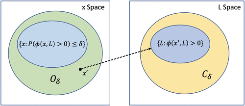
In the rest of this paper, we will refer to as the outer approximation set and as the uniform conditional event. A graphical illustration of and is shown in Figure 1.
As hinted in our earlier discussion that motivates Property 1, we shall focus on the case that L follows a multivariate regularly varying distribution (i.e. a multidimensional version of a power-law-type distribution). The definition of multivariate regular variation is provided in Section 5. In this case, to illuminate how the sets and can be constructed for different problems, we provide explicit expressions of them for two running examples in Table 1. In Section 5, we will illustrate how to construct and for more general settings.
Now, given and that satisfies Property 1, we define the conditionally sampled problem ():
Here, are independent and identically distributed (i.i.d.) samples generated from the conditional distribution .
We now present our main result of this section in Lemma 1, which validates () is an effective and sample efficient scenario approximation by incorporating (Calafiore and Campi 2006, theorem 2) and Property 1. The proof of Lemma 1 will be presented in Section 4.1.
Suppose that Property 1 is imposed and let be a given confidence level.
Let and be any integer that satisfies
(5)With probability at least , if the conditionally sampled problem () is feasible, then its optimal solution and
Let be any integer such that . Assume that the chance constraint problem () is feasible. Then, with probability at least , () is feasible and .
(Size of Conditionally Sampled Problem). The lower bound of the sample size given in (5) is not greater than , which is independent of δ. Therefore, Lemma 1 shows that the chance constraint problem () can be approximated by () with sample complexity bounded uniformly as , as long as Property 1 is satisfied.
(Feasibility of Conditionally Sampled Problem). In Lemma 1, part 1, the conditionally sampled problem () is feasible with high probability if there exists small δ such that () is feasible. In particular, we claim that
We next prove (6). For arbitrarily small , the feasible region for problem () is nonempty, and thus we can pick such that . If , then and thus . Therefore, by the independence of samples,
Letting , we conclude that (6) holds.
(Efficient Sampling Algorithm). Efficiently generating samples of when requires rare event simulation techniques. For example, when L is light-tailed, exponential tilting can be applied to achieve O(1) sample complexity uniformly in δ; when L is heavy-tailed, with the help of specific problem structure, one can apply importance sampling (Blanchet and Liu 2010) or Markov chain Monte Carlo (Gudmundsson and Hult 2014) to design an efficient sampling scheme. The specific structure of our salvage fund example results in being the complement of a box, which makes the sampling very tractable if the element of L are independent.
Even if the aforementioned rare event simulation techniques are hard to apply in practice, we can still apply a simple acceptance-rejection procedure to sample the conditional distribution . It costs samples of L on average to get one sample of because . Consequently, the total complexity for generating and solving is , which is still much more efficient than the scenario approach in Calafiore and Campi (2006), because it requires computational complexity for solving a linear programming problem with sampled constraints by the interior point method.
Although Property 1 seems to be restrictive at first glance, we are still able to construct the sets and for a rich class of functions , including the constraint function for the minimal salvage fund problem. As we shall see in the proof of Lemma 1, once and are constructed the sampled problem () is a tractable approximation to the problem (). We explain how to construct the sets and in the next section under some additional assumptions. These assumptions relate in particular to the distribution of L. It turns out that, if L is heavy-tailed, the construction of and becomes tractable.
4.1. Proof of Lemma 1
If Property 1 is satisfied, () is equivalent to
Let denote the risk level in the equivalent problem (7). The sampled optimization problem related to Problem (7) is given by
According to Calafiore and Campi (2006, corollary 1 and theorem 2), with probability at least , if the sampled problem () is feasible, then the optimal solution to problem () is feasible to the chance constraint problem (7). Because (7) and () are equivalent, the optimal solution to problem () is also feasible to (). The proof of the first part of the lemma is complete.
Now we turn to prove the second part of the lemma. The equivalence between () and (7) is still valid, so it is sufficient to compare the optimal values of (7) and (). By applying Calafiore and Campi (2006, theorem 2) again, we have with probability at least () is feasible and the value of () is no larger than the optimal value of
The proof is complete by using . Therefore, using for “value of,” .
5. Constructing Outer Approximations and Summary of the Algorithm
In this section, we come full circle with the intuition borrowed from rare event simulation explained at the beginning of Section 4. The scale-free properties of heavy-tailed distributions (to be reviewed momentarily) coupled with natural (polynomial) growth conditions (like the linear loss) given by the structure of the optimization problem, provide the necessary ingredients to show that the set has a probability that is of order .
In the discussion immediately following Property 1, we imagined that the uniform conditional set was of the form for as . However, Property 1 can still be enforced if this statement applies to L2 or any power of L. This is because power law-type decay (and more generally regular variation) is preserved under power transformations. We will provide assumptions that will enforce that regular variation properties can be applied when estimating the likelihood of the uniform conditional event.
We assume that the distribution of L is of multivariate regular variation. A definition that we now review. For background, we refer to Resnick (2013). Let denote all Radon measures on the space (recall that a measure is Radon if it assigns finite mass to all compact sets). If , then μn converges to μ vaguely, denoted by , if for all compactly supported continuous functions ,
L is multivariate regularly varying with limit measure .
Here are some intuitions behind the definition of multivariate regularly varying. Suppose that L is written in terms of polar coordinates, with R being the radius and Θ being a random variable taking values on the unit sphere. The radius has a one-dimensional regularly varying tail (i.e., we can write for a slowly varying function L and ). The angle Θ, conditioned on R being large, converges weakly (as ) to a limiting random variable. The distribution of this limit can be expressed in terms of the measure μ. For a recent application of multivariate regular variation in operations research, see Kley et al. (2016).
In this section, we present two methods for the construction of and satisfying Property 1. We mostly focus on our “scaling method” which is presented in Section 5.1, which is facilitated precisely by the scale-free property that we will impose on L. After showing the construction of the outer sets under the scaling method, we summarize the algorithm at the end of Section 5.1. We supply a lower bound guaranteeing a constant approximation for the output of the algorithm in Section 5.2. Our second method for outer approximation constructions is summarized in Section 5.3. This method is simpler to apply because is based on linear approximations; however, it is less general because it assumes that is jointly convex.
5.1. Scaling Method
We start by analyzing the feasible region when . Intuitively, if the violation probability has a strictly positive lower bound in any compact set, then will ultimately be disjoint with the compact set when . Thus, the set is expelled to infinity when in this case. is moving toward the direction that becomes small such that the violation probability becomes smaller. For instance, if x is one dimensional and is increasing in x, then is moving toward the negative direction. Consider the portfolio optimization problem as another example, in which as .
With such intuition, now we begin to construct the outer approximation set . To this end, we need to introduce an auxiliary function which we shall call a level function. We assume the existence of a level function in Assumption 2, and the level function needs to be explicitly computable to construct the outer approximation set .
We say that is a level function if
For any and , we have ,
The function π(x) is coersive, i.e., .
For a given level function π, we define its unit level set as .
There exists an explicitly computable level function π and its unit level set Π.
The unit level set Π is used to characterize the moving direction of as . The shape of Π is chosen in accordance with the moving direction of to reduce the size of to achieve better sample complexity. The outer approximation set is constructed as
Suppose that , then the level function π can be chosen as the Euclidean norm and Π can be chosen as the unit sphere in .
For the portfolio optimization problem, the level function can be chosen as in accordance with our intuition that , and the unit level set can be chosen as .
To analyze the asymptotic shape of the uniform conditional event , we connect the asymptotic distribution of L to the asymptotic distribution of . Keep in mind that we wish to preserve the scaling property of the tail of L, when considering , so that Property 1 can be ensured. We pick a continuous nondecreasing function such that to characterize the scaling rate of L. In addition, we pick another positive function to characterize the scaling rate of . Intuitively, the scaling function and should ensure the condition that the collection of probability measures of is tight. For the minimal salvage fund problem with fixed δ, as the deficit is asymptotically linear with respect to the salvage fund x and the loss L, we can simply pick in this problem. We next introduce two auxiliary functions and .
Let be two Borel measurable functions. We say (respectively, c) is the asymptotic uniform upper (respectively, lower) bound of over the unit level set if for any compact set ,
We would like to have lower and upper bounds and so that is of the order for every decision x, and in every direction l of the random vector L, whenever the norm of the latter is large (i.e., of the size ). A stronger assumption would have been to require an actual limit (rather than a liminf and a limsup), but this is not needed to provide big-O bounds for the complexity of our algorithm.
The functions and are used to define the event and , which serve as the inner and outer approximation of the event , where is the violation event at x.
For , let (respectively, ) be the ε-outer (respectively, inner) approximation event:
We now define . The following property ensures that the shape of Π is appropriate and is large enough; hence, is an outer approximation of .
There exist δ0 such that for any , we have an explicitly computable constant that satisfies
If the violation probability is easy to analyze, we will directly derive the expression of and verify Property 2. Otherwise, we resort to Lemma 2, which provides a sufficient condition of Property 2 by analyzing the asymptotic probability of the violation event as .
Suppose that Assumptions 1 and 2 hold. If there exists an asymptotic uniform lower bound function as given in (9b) and such that , then Property 2 is satisfied.
The high-level idea of Lemma 2 is to show that is disjoint from for small α. To this end, the asymptotic scaling (9b) is used to demonstrate that the violation probability is no less than , which is approximately equal to according to the regularly varying property of L. The detailed proof of Lemma 2 is deferred to Appendix A.1.
We impose the following Assumption 3 on the asymptotic uniform upper bound so that we can use the multivariate regular variation of L to estimate for large scaling factor α.
There exist an event with such that
In addition, there exist some such that is bounded away from the origin, that is,
Moreover, both S and have explicit expressions.
For the minimal salvage fund problem, because the deficit function is coordinate-wise nondecreasing with respect to the loss vector L, it is reasonable to assume that its asymptotic bound is also coordinate-wise nondecreasing. For this example, the closed form expression of and the detailed verification of all the assumptions are deferred to Proposition 2. Our next result summarizes the construction of the outer approximation sets.
Suppose that Property 2 and Assumption 3 are imposed. Then there exist such that the following sets
The main idea for proving Theorem 1 is as follows: If L lies in a “well-behaved” compact region, then by applying Assumption 3 and the asymptotic uniform lower bound (9b), the violation events is uniformly enclosed in . Otherwise L lies in the “ill-behaved” region . Combining these two cases inspires that definition of , and the probability of is because of and L is regularly varying. The detailed proof of Theorem 1 is deferred to Appendix A.1.
With the aid of Lemma 1 and Theorem 1, we provide an algorithm for approximating () in which the sampled optimization problem is bounded in .
(Scenario Approach with Optimal Scenario Generation)
input: Risk tolerance parameter δ, confidence level β, and all the elements and constants appearing in Property 2 and Assumption 3, including level function π or unit level set Π, constant , scaling function h, and explicit expression of and S.
5.2. Constant Approximation Guarantee
In Section 5.2, our objective is to show that the output of the previous algorithm is guaranteed to be within a constant factor of the optimal solution to () with high probability, uniformly in δ.
We shall work under the setting of Theorem 1, so we enforce Property 2 and Assumptions 3. We want to show that there exist some constant independent of δ, such that with high probability. This indicates that our result guarantees a constant approximation to () for regularly varying distributions (under our assumptions) in O(1) sample complexity when with high probability.
Note that is meaningful only if . We assume that the outer approximation set is good enough such that the following natural assumption is valid.
There exist such that .
The previous assumption will typically hold if c has strictly positive entries. Theorem 1 and the form of guarantee that the norm of the optimal solution of () grows in proportion to , so we also assume the following scaling property for .
There exist a function such that for every compact set , we have
In addition, is continuous in one.
Assumption 5 is satisfied by both running examples. For the portfolio optimization problem, we have , thus . For the minimal salvage fund problem, we have such that and .
We define the following optimization problem, which will serve as an asymptotic upper bound of in stochastic order when :
Let be a given confidence level and be a fixed integer that satisfies (5). If Assumptions 4 and 5 are enforced, and () satisfies Slater’s condition with probability one, then there exist and such that
In Theorem 2, the Slater’s condition (see section 5.2.3 in Boyd and Vandenberghe (2004) for reference) can be verified directly on the problem (). This condition is satisfied in the salvage fund problem by standard linear programming duality. We also remark that Assumptions 4 and 5 only require the existence rather than the explicit knowledge of and function .
5.3. Linear Approximation Method
Suppose that the constraint function is jointly convex in (x, l), and L is multivariate regularly varying. We will develop a simpler method in this section to construct the outer approximation set and the uniform conditional event .
We first introduce a crucial assumption in the construction of and .
There exist a convex piecewise linear function of the form
The inequality ;
There exist some constant such that if .
If itself is a piecewise affine function, then Assumption 6 is satisfied by simply taking . For general jointly convex functions, the following lemma verifies Assumption 6 if has a compact zero sublevel set.
If the constraint function is convex and twice continuously differentiable, and it has a compact zero sublevel set , then Assumption 6 is satisfied.
With Assumption 6 enforced, we are now ready to provide our main result in this section to fully summarize the construction of and .
If Assumptions 1 and 6 hold, we can construct and that satisfy Property 1 as
6. Verifying the Assumptions in Examples
In this section, we verify the elements required to apply our algorithm. We provide explicit expressions for sets and in the statement of the propositions. The detailed verification process and the steps for constructing sets and are presented as the proofs in Appendix A.2.
6.1. Portfolio Optimization with VaR Constraint
In this section, we will verify that Theorem 1 is applicable to an equivalent form of the portfolio optimization problem (2).
The portfolio optimization problem (1) satisfies all assumptions required by Theorem 1, such that the sets and admit the following explicit expressions:
6.2. Minimal Salvage Fund
The key observation to solve the minimal salvage fund problem (3) is the following lemma, which provides a closed form piecewise linear expression for the constraint function .
In the minimal salvage fund problem (3), we have
Now we prove that Theorem 3 is applicable to the minimal salvage fund problem (4).
The minimal salvage fund problem (3) satisfies all assumptions required by Theorem 3, such that the sets and admit the following explicit expressions:
6.3. Quadratic Model
In this section, we consider a model with a quadratic control term in x as an additional example. Suppose that the constraint function is defined as
Consider the chance constraint optimization model with constraint function defined as (12).
If Q is a positive semidefinite matrix and L has a positive density, there exist some δ such that the problem is infeasible.
If Q has a negative eigenvalue and L is multivariate regularly varying, the model satisfies all the assumptions required by Theorem 1.
7. Numerical Experiments
To empirically study the computational complexity and compare the quality of the solutions, in this section, we conduct numerical experiments for two scenario generation algorithms:
The efficient scenario generation approach proposed in this paper (abbreviated as Eff-Sc)
The scenario approach in Calafiore and Campi (2006) (abbreviated as CC-Sc)
In Section 7.1, we present the results for the portfolio optimization problem. In Section 7.2, we present the results for the minimal salvage fund problem. The numerical experiment is conducted using a Laptop with a 2.2-GHz Intel Core i7 CPU, and the sampled linear programming problem is solved using CVXPY (Diamond and Boyd 2016) with the MOSEK solver (MOSEK ApS 2020).
7.1. Portfolio Optimization with VaR Constraint
First, we present the parameter selection and the implement details for the numerical experiment of portfolio optimization problem (1). Suppose that there are d = 10 assets to invest, and the parameters of the problem are chosen as follows:
The mean return vector is .
The random variable Lj are i.i.d. with Pareto cumulative distribution function , for .
The parameter .
The loss threshold η = 1,000.
Now we explain the implementation detail of Eff-Sc. Recall the expression of and from Proposition 1, which involves the analytically unknown quantity . Because quantile estimation is much more computationally efficient than solving the sampled optimization problem, we generate samples of L to estimate a confidence interval of with large enough confidence level , and we denote the resulting confidence interval by . We replace the expressions of and by their sampled version conservative approximations, that is,
The value of is also estimated using the generated samples. We compute the required number of samples using Lemma 1, and the samples of is generated via acceptance-rejection.
In Figure 2, we compare the efficiency between Eff-Sc and CC-Sc. Figure 2(a) presents the required number of samples for both algorithms, in which one can quickly remark that Eff-Sc requires significantly fewer samples than CC-Sc, especially for the problems with small δ. In Figure 2(b), we compare the running time for both models. Whereas Eff-Sc costs slightly more time for δ around 0.1 due to the overhead cost of computing and , the computational time stays nearly constant uniformly in δ, indicating that Eff-Sc is a substantially more efficient algorithm than CC-Sc.

Notes. (a) Terms of the required number of samples. (b) Used CPU time. We test
Finally, we compare Eff-Sc and CC-Sc for the optimal values of the sampled problems and the violation probabilities of the optimal solutions. Because both methods require generating random samples, the generated solutions are also random. Thus, the optimal values and the violation probabilities are also random. To compare the distributions of the random quantities, we conduct 103 independent experiments. In each experiment, we execute both algorithms and get two solutions, then we evaluate the solutions’ violation probabilities using 106 samples of L. We use boxplots (McGill et al. 1978) to depict the samples’ distribution through their quantiles. A boxplot is constructed of two parts: a box and a set of whiskers. The box is drawn from the 25% quantile to the 75% quantile, with a horizontal line drawn in the middle to denote the median. Two whiskers indicate 5% and 95% quantiles, respectively, and the scatters represent all the rest sample points beyond the whiskers.
In Figure 3, we present (a) the optimal values and (b) the violation probabilities. One can quickly remark from Figure 3(a) that the optimal value of Eff-Sc is stochastically larger than the optimal value of CC-Sc, whereas Figure 3(b) indicates that the optimal solutions produced by both methods are feasible for all the 103 experiments. Overall, with both methods successfully and conservatively approximating the probabilistic constraint, Eff-Sc is more computationally efficient and less conservative, producing solutions with better objective values than its counterpart.
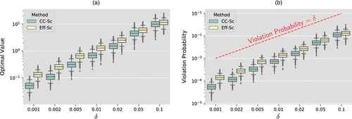
Notes. (a) Optimal value. (b) Solutions’ violation probabilities. Here , and the box plots are generated using 1,000 experiments.
7.2. Minimal Salvage Fund
In this section, we conduct a numerical experiment for the minimal salvage fund problem (3). In the experiment, we pick to test the performance of the problem in different dimensions.
For each fixed d, the parameters of Problem (3) are chosen as follows:
The matrix where if and otherwise .
The vector where mj = 10 for each j.
The random variables Lj are i.i.d. with Pareto cumulative distribution function , for .
Recall the explicit expressions for sets and from Proposition 2. To solve the conditionally sampled problem (), it remains to sample and compute , the required number of samples. When δ is small, when , solving the optimization problem () costs much more time than simulating , despite that a simple acceptance rejection scheme is applied to sample in our experiments. We fix the confidence level parameter and set , and then we can compute by the first part of Lemma 1.
Similar to Figure 2 of the portfolio optimization problem, we compare the efficiency between Eff-Sc and CC-Sc for different d and δ in Figure 4, in terms of (a) the required number of samples and (b) the CPU time for solving the sampled approximation problem. We observe that the Eff-Sc has uniformly smaller sample complexity and computational complexity than CC-Sc, where the superiority becomes significant for small δ. In particular, the required number of samples and the used CPU time are bounded for Eff-Sc, whereas they quickly deteriorate for CC-Sc when δ becomes smaller. It is also worth noting that Eff-Sc is consistently more efficient than CC-Sc for all the tested dimensions.
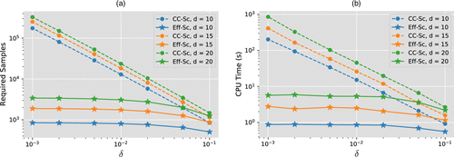
Notes. (a) Required number of samples. (b) Used CPU time. We test and
Finally, we compare optimal values of the sampled problems and violation probabilities of the optimal solutions in Figure 5. We present in Figure 5(a) the optimal values and in Figure 5(b) the violation probabilities, with fixed dimension d = 15 (we provide additional results for d = 5 and d = 10 in Appendix C.3). One can quickly remark from Figure 5(a) that the optimal value of Eff-Sc is stochastically smaller than the optimal value of CC-Sc, whereas Figure 5(b) indicates that the optimal solutions produced by both methods are feasible for all the 103 experiments. Therefore, we are able to draw the same conclusion as we have from the portfolio optimization experiment: Eff-Sc efficiently produces less conservative solutions.
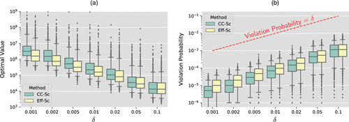
Notes. (a) Optimal value. (b) Solutions’ violation probabilities. Here d = 15, , and the box plots are generated using 1,000 experiments.
The authors thank Alexander Shapiro for helpful comments.
Appendix A. Proofs of Technical Results
A.1. Proofs for Section 5
We will derive an expression of to ensure that for δ small enough. Because of Assumption 2, for any , there exist some δ small enough such that . Therefore, it suffices to prove that and are disjoint. In other words,
Let ε be a positive number such that . Pick the set K in (9b) as a compact set such that . It follows from Inequality (9b) that there exist a constant α1 such that
Therefore, for any , we have
Recall that L is regularly varying from Assumption 1,
Therefore, there exist a number α2 such that
The right-hand side of (A.4) is nondecreasing in α. Thus, if for any , there exists satisfying
Substituting (A.5) into (A.3), we have
Moreover, Assumption 2 guarantees the existence of δ2 such that
Consequently (A.1) is proved with . □
We construct the uniform conditional event that contains all the Vx for . Because of Definition (9) and , there exists δ0 such that for all ,
For any , there exists an such that . Consequently, it follows from (A.6) that
Applying Assumption 3 yields that
Recall that K is a ball in (thus, ) and that from Assumption 3, it follows that . Consequently, whenever for some , we either have implying , or we have . Summarizing these two scenarios,
Thus, we define the conditional set as
It remains to analyze the probability of the uniform conditional event . As L is multivariate regularly varying,
Recalling, and invoking Property 2, we get
Hence, the proof is complete. □
Using Lemma 1, we immediately have it remains to show that there exist such that .
For simplicity, in the proof, we will use as a shorthand for , the random variable with conditional distribution of L given . By a scaling of x by a factor in (), we have an equivalent optimization problem:
For any compact set , because L is multivariate regularly varying,
Thus, . As the limiting measure is a probability measure, the family is tight and consequently follows directly from the vague convergence (Resnick 2013). Consequently, because all the samples are i.i.d, we also have
Now we define a family of deterministic optimization problem, denoted by (), which is parameterized by as follows:
Then, there exist a compact set such that
Problem () satisfies Slater’s condition if ;
The probability for all ;
For every and , due to the Slater’s condition, there exists a feasible solution such that . Because is continuous in l, there exists an open neighborhood U around such that . Such a feasible solution x and neighborhood U exist for every .
There exists a finite open cover of E1 due to its compactness. Let be the corresponding feasible solutions to the open cover .
From Assumption 5, there exists such that for all , we have
Therefore, by the triangle inequality, it follows that if ,
Consequently, xj is a feasible solution for Optimization Problem (A.7) if , which further implies that . As a result, we have
Note that . Therefore, let
It follows that
The statement is concluded by using the union bound, combining the lower bound together with the upper bound implied by Lemma 1 and Theorem 1, hence obtaining factor . □
Without loss of generality, assume that R is an integer such that
Let , and let be the integer lattice points in . In addition, let and for , then define . Because the function is convex, we can invoke the supporting hyperplane theorem to deduce that for , and consequently . In addition, because at the boundary of the cube , there exist a constant C1 such that for and for , for all . Therefore, with being the maximum of the aforementioned linear functions, we have , and we also have that implies .
Define . We can conclude the property of as follows: (1) is a piecewise linear function of form , where ; (2) ; and (3) implies . To complete the proof, it remains to verify for the second statement of Assumption 6.
As implies , it suffices to prove that there exist some universal constant such that for all . For an arbitrary point , there exist a lattice point such that Next, because is twice continuously differentiable, the gradient is Lipschitz over with Lipschitz constant denoted by . Therefore, for any ,
The proof is now complete. □
Because , the probability constraint implies that , which further implies for . Therefore, we have for , which implies .
Then, consider and . It follows from the second statement of Assumption 6 that implies that . Thus, there exist an index i such that . As implies that , so
Therefore, the condition set can be constructed as
Thus, as the distribution is regularly varying in dimension one for each j, we have , completing the proof. □
A.2. Proofs for Section 6
Let and . The unit level set is . Let and , it follows that . In view of the inequalities and when , we choose the asymptotic uniform bounds as
Furthermore, by definition, we construct two approximation sets as
With all the elements that we have already defined, Assumption 1 follows directly from the assumption on distribution of L. Now we turn to verify Assumption 2. As due to the definition of , it suffices to prove that . In view of , we have
Consequently, we have . Taking limit for , we conclude that .
As Assumptions 1 and 2 are both satisfied, and we also have , Property 2 is verified due to Lemma 2. In addition, if , we have is bounded away from the origin. Thus, Assumption 3 is verified with .
Finally, we provide closed form expressions for and . Define ; then it follows that , and By setting , we get the expression in the statement of the theorem. □
We start by showing some properties of . Because Q is a nonnegative matrix and the row sum is less than one, it is a substochastic matrix, and all of its eigenvalues must be less than one in magnitude. This further implies (1) is invertible, and (2) is a nonnegative matrix with strictly positive diagonal terms.
Notice that is the unique vector such that . Let be the optimal solution of
We have , and we multiply the nonnegative matrix on both sides, yielding . Obviously, let such that (y, b) is a feasible solution to above problem. Obviously, it follows from that ; thus, (y, b) is also optimal, which completes the proof. □
Assumption 1 follows directly from the assumptions of the example. Now we turn to verify Assumption 6. Using Lemma 4, we define . Therefore, Assumption 6 is satisfied with n = d, and C = 0. Plugging the previous values into the expressions of and given in Theorem 3, we get the expressions shown in the statement of the proposition. □
The following lemma is used in the proof of Proposition 3.
There exist sets with positive Lebesgue measure such that for any with , there exist some .
Let denote the unit vector on the jth coordinate in for . Fix with , define θj be the angle between z and , which satisfies . Because we have , so there exist some i such that ; thus, . Then, define
We have either or . Thus, the proof is complete. □
For the first statement, because and , and invoking the assumption that L has a positive density:
For the second statement, Assumption 1 is easy to verify. Notice that for all , so we pick the scaling rate function as and . Let denote the maximal eigenvalue of Q, and denote the minimal eigenvalue of Q. The rest of the proof will be divided into two cases.
Case 1 (): We pick the unit level set as . Because , Assumption 2 is verified. Next, we directly show Property 2 instead of using Lemma 2. For any , we have
Thus, can be chosen such that , and . As a result, Property 2 is verified. We next turn to derive the asymptotic uniform bound . Observing that
Case 2 (): The unit level set Π is chosen as an unbounded set , and we have . For any , we have
Thus, we can pick an that satisfies Property 2. Now, is bounded by
Appendix B. Importance Sampling for Multivariate Regularly Varying Distribution
B.1. Multivariate Regularly Varying Distribution with Gaussian Copula
In this section, we assume that the correlation structure of the random vector L is characterized by Gaussian Copula.
Let be the standard univariate Gaussian cumulative distribution function (CDF), and be the joint CDF of multivariate Gaussian CDF with mean of zero, variance of one, and covariance matrix of Σ. The Gaussian Copula is defined as Suppose that the random vector L has marginal CDF for , we assume that has joint CDF .
(Sampling of Multivariate Regularly Varying Distribution with Gaussian Copula)
Input: The covariance matrix of Gaussian Copula Σ, the marginal CDFs .
1 Apply Cholesky decomposition or singular value decomposition to compute the matrix A such that .
2 Sample a d-dimensional multivariate standard normal vector Z, compute the linear transform .
3 For each , compute .
In the importance sampling algorithm developed later, we need to sample the random vector L conditional on the value of one coordinate, for example, Li = li. Without loss of generality, we assume that the value of the last coordinate is given, and the covariance matrix Σ admits the blockwise representation where , , and . Suppose that X is a random vector with normal distribution , then the conditional distribution of given Xd = xd is jointly normal distributed with mean and covariance . In Algorithm B.2, we describe the conditional sampling method for L.
(Sampling of Multivariate Regularly Varying Distribution with Gaussian Copula Conditional on Ld = ld)
Input: The covariance matrix of Gaussian Copula Σ, the marginal CDFs , the conditional value of the last coordinate Ld = ld.
1 Map the observation into the Gaussian space: .
2 Sample a d − 1-dimensional multivariate normal vector , with mean and covariance .
3 For each , compute .
B.2. Importance Sampling
In this section, we present an importance sampling method to sample from the conditional distribution , where is the uniform conditional event.
B.2.1. Minimal Salvage Fund.
Recall from Proposition 2 that the uniform conditional event for the minimal salvage fund problem is To simplify the notation, let us define for . It follows that for .
The algorithm is a combination of acceptance rejection and importance sampling. Suppose that is the probability measure corresponding to the random vector L, then the target measure corresponding to the conditional distribution can be expressed as
Now we describe how to sample from the proposal distribution with importance sampling. For each fixed , the conditional distribution can be sampled using the importance sampling: We first sample Li conditional on by the inverse CDF method and then apply Algorithm B.2 to sample Lj for conditional on Li. The resulting random vector L has probability measure . Then, if we uniformly sample the random index i from instead of using the fixed index, the proposal distribution becomes
The likelihood ratio is
The proposal distribution guarantees that there exist at least an index i such that ; thus, we have and . In addition, the definition of implies that . Consequently, the likelihood ratio is upper bounded by d.
To conclude this section, we summarize the detail of the importance sampling in Algorithm B.3.
(Importance Sampling Algorithm for Minimal Salvage Fund Problem)
Input: The covariance matrix of Gaussian Copula Σ, the marginal CDFs , the risk level of tolerance δ.
1 Uniformly sample a random index
2 Sample a uniform random variable . Set
3 Apply Algorithm B.2 to sample the rest coordinates Lj for conditional on the value of Li.
4 Sample a uniform random variable .
5 If , output ; otherwise, return to step 1.
B.2.2. Portfolio Optimization with VaR Constraint.
Recall from Proposition 1 that the uniform conditional event for the portfolio optimization problem is It is not hard to see that
Because the target distribution is still the likelihood ratio is
To conclude this section, we summarize the detail of the importance sampling in Algorithm B.4.
(Importance Sampling Algorithm for Portfolio Optimization with VaR Constraint)
Input: The covariance matrix of Gaussian Copula Σ, the marginal CDFs , the risk level of tolerance δ.
1 Sample a random index with probability propotional to , where
2 Sample a uniform random variable . Set
3 Apply Algorithm B.2 to sample the rest coordinates Lj for conditional on the value of Li.
4 Sample a uniform random variable .
5 If (i.e., and , output ; otherwise, return to step 1.
Appendix C. Additional Numerical Results
C.1. Portfolio Optimization with Dependent Loss
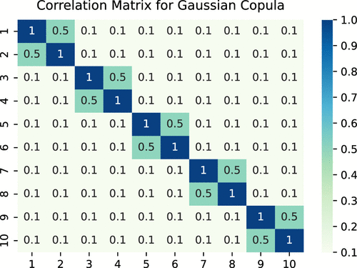
In this section, we conduct additional numerical experiments for the portfolio optimization problem (2). We still consider the portfolio optimization problem with d = 10 assets and use the same mean return vector μ and loss threshold η as Section 7.1. Although we also assume the same marginal distribution for the loss vector L, we apply the Gaussian Copula (see Appendix B.1) to impose the dependence structure between different coordinates of L. In particular, we assume the correlation matrix of Gaussian Copula as in Figure C.1.
To solve the change constraint problem using Eff-Sc. We adopt the same construction of and as Section 7.1 and compute the required number of samples using Lemma 1. The samples of is generated via the importance sample method (see Algorithm B.4 for detail).
In Figure C.2, we compare the efficiency between Eff-Sc and CC-Sc. As shown in Figure C.2(a), the required number of samples for Eff-Sc is substantially less than CC-Sc, especially when δ is small. In Figure C.2(b), we compare the running time for both models. We remark that the computational time for Eff-Sc stays nearly constant for different δ, and that Eff-Sc needs less time to solve than CC-Sc for small δ.
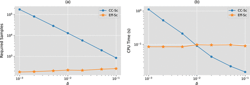
Notes. (a) Required number of samples. (b) Used CPU time. We test
In Figure C.3, we compare the optimal value and the conservativeness of the solutions generated by Eff-Sc and CC-Sc. From the figure, we can conclude that the solutions for Eff-Sc and CC-Sc are both feasible, and the Eff-Sc solution is less conservative with better optimal value.

Notes. (a) Optimal value. (b) Solutions’ violation probabilities. Here , and the box plots are generated using 1,000 experiments.
C.2. Minimal Salvage Fund with Dependent Loss
In this section, we test the performance of the minimal salvage fund problem (2) in which the loss vector L has dependent structure characterized by the Gaussian copula.
In the experiment, we fixed d = 10, and use the same parameters Q and m and the same marginal distribution of Lj as introduced in Section 7.2. We assume that the dependence structure of different coordinates of L is prescribed by the Gaussian Copula with correlation matrix shown in Figure C.1.
In Figure C.4, we compare the efficiency between Eff-Sc and CC-Sc for solving the minimal salvage fund problem. In particular, we compare the required number of samples in Figure C.4(a) and the total required CPU time in Figure C.4(b). Despite slightly larger CPU time for Eff-Sc for large δ, the CPU time for Eff-Sc becomes significantly smaller than CC-Sc when , and the required number of samples for Eff-Sc is also universally smaller.
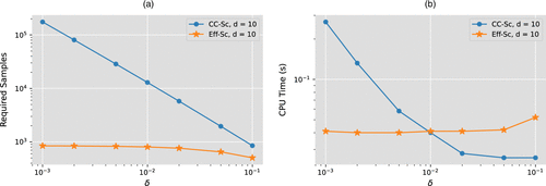
Notes. (a) Required number of samples. (b) Used CPU time. We test d = 10 and
In Figure C.5, we also compare the quality of the solutions generated by Eff-Sc and CC-Sc. Once again, we found that the solutions generated by Eff-Sc are less conservative with better optimal value on average.
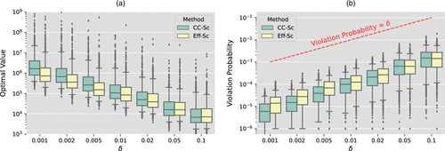
Notes. (a) Optimal value. (b) Solutions’ violation probabilities. Here d = 10, , and the box plots are generated using 1,000 experiments.
C.3. Minimal Salvage Fund for d = 5 and d = 10
In this section, we demonstrate the quality of the solutions produced by Eff-Sc is better than CC-Sc when the dimension of the problem is d = 5 or d = 10. See Figure C.6 for dimension d = 5 and Figure C.7 for d = 10.

Notes. (a) Optimal value. (b) Solutions’ violation probabilities.
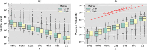
Notes. (a) Optimal value. (b) Solutions’ violation probabilities.
References
- (2008)
Solving chance-constrained stochastic programs via sampling and integer programming . Chen Z-L, Raghavan S, eds. State-of-the-Art Decision-Making Tools in the Information-Intensive Age (INFORMS), 261–269.Link, Google Scholar - (2019) A chance constrained based formulation for dynamic multiplexing of eMBB-URLLC traffics in 5G new radio. Proc. Internat. Conf. on Information Networking (IEEE, New York), 108–113.Google Scholar
- (2010) A model for dynamic chance constraints in hydro power reservoir management. Eur. J. Oper. Res. 207(2):579–589.Google Scholar
- (2016) Chance-constrained problems and rare events: An importance sampling approach. Math. Programming 157(1):153–189.Google Scholar
- (2000) Robust solutions of linear programming problems contaminated with uncertain data. Math. Programming 88(3):411–424.Google Scholar
- (2002) Robust optimization: Methodology and applications. Math. Programming 92(3):453–480.Google Scholar
- (2004) The price of robustness. Oper. Res. 52(1):35–53.Link, Google Scholar
- (2010) Efficient importance sampling in ruin problems for multidimensional regularly varying random walks. J. Appl. Probability 47(2):301–322.Google Scholar
- (2009) An exact solution approach for portfolio optimization problems under stochastic and integer constraints. Oper. Res. 57(3):650–670.Link, Google Scholar
- (2004) Convex Optimization (Cambridge University Press, Cambridge, UK).Google Scholar
- (2005) Uncertain convex programs: Randomized solutions and confidence levels. Math. Programming 102(1):25–46.Google Scholar
- (2006) The scenario approach to robust control design. IEEE Trans. Automated Control 51(5):742–753.Google Scholar
- (1958) Cost horizons and certainty equivalents: An approach to stochastic programming of heating oil. Management Sci. 4(3):235–263.Link, Google Scholar
- (2019) Efficient rare-event simulation for multiple jump events in regularly varying random walks and compound Poisson processes. Math. Oper. Res. 44(3):919–942.Link, Google Scholar
- (2010) From CVaR to uncertainty set: Implications in joint chance-constrained optimization. Oper. Res. 58(2):470–485.Link, Google Scholar
- (2016) CVXPY: A Python-embedded modeling language for convex optimization. J. Machine Learn. Res. 17(83):1–5.Google Scholar
- (2001) Systemic risk in financial systems. Management Sci. 47(2):236–249.Link, Google Scholar
- (2013) Modelling Extremal Events: For Insurance and Finance, vol. 33 (Springer Science & Business Media, Boston).Google Scholar
- (2008) Municipal bond fairness act. 110th Congress, 2d Session, House of Representatives, Report, 110–835.Google Scholar
- (2014) Markov chain Monte Carlo for computing rare-event probabilities for a heavy-tailed random walk. J. Appl. Probability 51(2):359–376.Google Scholar
- (1967) Chance-constrained programming with 0-1 or bounded continuous decision variables. Management Sci. 14(1):34–57.Link, Google Scholar
- (2021) Learning-based robust optimization: Procedures and statistical guarantees. Management Sci. 67(6):3447–3467.Link, Google Scholar
- (2011) Sequential convex approximations to joint chance constrained programs: A Monte Carlo approach. Oper. Res. 59(3):617–630.Link, Google Scholar
- (2016) Risk in a large claims insurance market with bipartite graph structure. Oper. Res. 64(5):1159–1176.Link, Google Scholar
- (2012) On mixing sets arising in chance-constrained programming. Math. Programming 132(1–2):31–56.Google Scholar
- (2005) Probabilistically constrained linear programs and risk-adjusted controller design. SIAM J. Optim. 15(3):938–951.Google Scholar
- (2016) Solving chance-constrained optimization problems with stochastic quadratic inequalities. Oper. Res. 64(4):939–957.Link, Google Scholar
- (2014) A branch-and-cut decomposition algorithm for solving chance-constrained mathematical programs with finite support. Math. Programming 146(1–2):219–244.Google Scholar
- (2008) A sample approximation approach for optimization with probabilistic constraints. SIAM J. Optim. 19(2):674–699.Google Scholar
- (2010) An integer programming approach for linear programs with probabilistic constraints. Math. Programming 122(2):247–272.Google Scholar
- (1978) Variations of box plots. Amer. Statist. 32(1):12–16.Google Scholar
MOSEK ApS (2020) MOSEK fusion API for Python. Retrieved September 10, 2020, https://docs.mosek.com/9.2/pythonfusion.pdf.Google Scholar- (2006a) Convex approximations of chance constrained programs. SIAM J. Optim. 17(4):969–996.Google Scholar
- (2006b) Scenario approximations of chance constraints. Probabilistic and Randomized Methods for Design Under Uncertainty (Springer, Berlin), 3–47.Google Scholar
- (2020) Solving chance-constrained problems via a smooth sample-based nonlinear approximation. SIAM J. Optim. 30(3):2221–2250.Google Scholar
- (1970) On probabilistic constrained programming. William Kuhn H, ed. Proc. Princeton Sympos. on Math. Programming, vol. 113 (Princeton University Press, Princeton), 138.Google Scholar
- (2003) Probabilistic programming. Handbook Oper. Res. Management Sci. 10:267–351.Google Scholar
- (2013) Extreme Values, Regular Variation and Point Processes (Springer, Berlin).Google Scholar
- (1971) Constructing sets of uniformly tighter linear approximations for a chance constraint. Management Sci. 17(11):736–749.Link, Google Scholar
- (2022) Optimization under rare chance constraints. SIAM J. Optim. 32(2):930–958.Google Scholar
- (2012) Is tail-optimal scheduling possible? Oper. Res. 60(5):1249–1257.Link, Google Scholar
- (2014) A branch-and-cut method for dynamic decision making under joint chance constraints. Management Sci. 60(5):1317–1333.Link, Google Scholar