Externalities in Queues as Stochastic Processes: The Case of FCFS M/G/1
Abstract
Externalities are the costs that a user of a common resource imposes on others. In the context of an FCFS M/G/1 queue, where a customer with service demand arrives when the workload level is , the externality is the total waiting time that could be saved if this customer gave up on their service demand. In this work, we analyze the externalities process . It is shown that this process can be represented by an integral of a (shifted in time by v) compound Poisson process with a positive discrete jump distribution, so that is convex. Furthermore, we compute the Laplace-Stieltjes transform of the finite-dimensional distributions of and its mean and auto-covariance functions. We also identify conditions under which a sequence of normalized externalities processes admits a weak convergence on equipped with the uniform metric to an integral of a (shifted in time by v) standard Wiener process. Finally, we also consider the extended framework when v is a general nonnegative random variable which is independent from the arrival process and the service demands. Our analysis leads to substantial generalizations of the results presented in the existing literature.
Funding: This research was supported by the European Union’s Horizon 2020 research and innovation programme [Marie Skłodowska-Curie Grant Agreement 945045] and the NWO Gravitation project NETWORKS [Grant 024.002.003].
1. Introduction
Consider a conventional M/G/1 queueing system that is served according to the first-come, first-served (FCFS) discipline, with arrival rate and with the service distribution given by . Assume that the queue is stable, and let the workload level at time t = 0 be (say) minutes. Denote the workload at time by , and let Ti be the arrival time of the ith customer. The main objective of this paper is to analyze the aggregate effect of an additional customer, who has arrived at time t = 0 with a service requirement of size , on the waiting times of all other customers. In other words, we are interested in the distribution of the externality:
Thus, the externality E(x, v) is to be interpreted as the total waiting time that could be saved if the additional customer reduced their service requirement from to zero. To the best of our knowledge, Haviv and Ritov (1998) is the only existing paper that analyzes E(x, v). In Haviv and Ritov (1998), it was shown that if (i) v is a random variable that is independent from the arrival process and the service requirements of the customers, and (ii) v is distributed according to the stationary distribution of the workload process, then the mean of E(x, v) is given by
Whereas Haviv and Ritov (1998) focused on computing the mean externality (under the specific condition mentioned previously), we have managed to develop a full probabilistic analysis of E(x, v). In this context it is important to notice that
The main contribution of this work lies in an extensive analysis of that, in the remainder of this paper, we refer to as the externalities process. Specific open questions that we have managed to solve in the current paper are as follows:
What can be said about the distribution of the externalities in a nonstationary FCFS M/G/1 queue? As it turns out, the externalities process can be represented by an integral of a compound Poisson process that is shifted in time by an amount v. Importantly, this compound Poisson process is defined on the same probability space as the one on which our model is defined.
Observe that the expected value in (2) is convex in x, which indicates that the marginal effect of extra workload on the customer population is increasing. Is it possible to extend this result by showing convexity of the externalities process? The answer is affirmative, where we also provide an explicit representation of the corresponding right-derivative.
Is there a systematic way to evaluate the moments of the externality ? To this end, we derive the Laplace-Stieltjes transform (LST) of the finite-dimensional distributions of the externalities process , from which the moments follow. In particular, we provide closed-form formulae for the auto-covariance and auto-correlation functions of . Remarkably, it is shown that when v is fixed, then the auto-correlation does not depend on the stochastic ingredients of the model, that is, the arrival rate and service distribution.
Is it possible to approximate the distribution of the externalities in some asymptotic regime? We show that, under an appropriate scaling, there is convergence of to a specific Gaussian limiting process. The convergence takes place as the arrival rate tends to infinity and the service distribution is well behaved; for example, it tends to zero in an appropriate way.
1.1. Motivation
We proceed by discussing the relevance of our results and their applicability in an operational context. We do so by distinguishing three strands of application domains.
1.1.1. Choice of a Management Scheme.
In the introduction of their paper, Haviv and Ritov (1998, p. 580) discuss various applications of the externalities setup that they analyze: airplanes taking off from a runway, commuters crossing a bridge, jobs sharing a common CPU, and messages being routed through a common data network. Their motivation for studying the distribution of externalities is as follows. In the first place, they argue that “a zero profit operator who charges users for the use of a common facility usually likes to do so in accordance with the congestion costs that they impose on others.” This aligns with results in, for example, Ha (2001), Haviv (2014), Haviv and Oz (2018a, b), and Jacobovic (2022b), where various relations between optimal queue regulation schemes and externalities are revealed. Then, they point out that there are various policies of managing a queueing system (e.g., by implementing different service disciplines). Correspondingly, different management policies may result in different amounts of externalities imposed by the same user. This leads them to the conclusion that “the resulting pricing mechanism can serve as an additional criterion for deciding which management scheme to adopt.” A general account of externalities in a queueing context is given in Hassin and Haviv (2003), as well as various other connections between queueing and game theory.
1.1.2. Queues with Discretionary Services.
Recently, there has been a growing interest in queueing models with customers who themselves choose their service durations (see Feldman and Segev (2022a) and Jacobovic (2022b) and the references therein). When considering single-server queues with a nonpreemptive service discipline, the customer who gets service does not care about the increasing costs of the waiting customers behind them, thus yielding a resource allocation which is inefficient from a social point of view. To restore social efficiency, a social planner may want to impose some sort of regulation. For example, the planner may decide on a price function that tells every customer how much they are going to pay for every service duration to be purchased. A price function will be optimal if it makes the customers behave as they should according to the socially optimal resource allocation. A reasonable price mechanism amounts to requiring every customer to pay for the expected cost that is enforced on the others due to their service requirement.
Jacobovic (2022b) considered a model of a single-server queue with customers who arrive according to a Poisson process and dynamically choose their service durations, showing that when the social planner is restricted to choose a price function which is determined by the service requirement only, then the optimal price function internalizes the (expected) externalities. It is an open problem (Jacobovic 2022a) whether a similar phenomenon occurs when the social planner may choose a price function that depends on the state of the queue. If the answer to this question is affirmative and the social planner observes the workload level at the onset of every service duration, then the optimal price function is equal to , with v the initial workload at the start of the service and x the corresponding service requirement. As is shown in the present paper, this would reduce the search for the optimal price function to the parametric family of quadratic functions in x which are also linear in v.
Similarly, in another possible scenario a social planner observes the number of waiting customers at the start of every service, but they do not see the customers’ service requirements (Haviv 2014, section 3). In this case, the conjectured optimal price function is the conditional expectation of given the available information at the start of the service. Once more, our results imply that this conditional expectation is quadratic in x and linear in the number of waiting customers at the time of the start of the service.
1.1.3. Queues with a Proactive Service Discipline.
Consider an emergency room with a single specific bed that is reserved for patients with special needs, for example, those who arrive because of strokes or heart attacks. We refer to these patients as urgent, whereas the patients who arrive due to other reasons are called regular. The special bed might be useful also for regular patients, whereas the urgent ones can be treated only in the special bed. Hence, a nontrivial question is as follows: If there are many regular patients and no urgent patients, should the regular patients be allowed to use the special bed? Doing so is evidently beneficial to the regular patients, but it is also possible that immediately after allocating a regular patient to the special bed, a batch of urgent patients arrives whose treatments will be delayed.
Now, assume that the urgent patients arrive according to a Poisson process with rate λ and their service requirements are independent and identically distributed (i.i.d.) random variables with a distribution function that are independent from the arrival process. Then, observe that is equal to the total damage that is caused to the urgent patients due to an allocation of a regular customer into the special bed for x minutes once it is empty. Clearly, the decision maker could benefit from the distributional properties of that we establish in the present paper.
The previous example connects our work with server-allocation problems in multiclass queues. Recent progress in this direction can be found in Chan et al. (2021), Hu et al. (2022), Huang et al. (2015), and Liu et al. (2022).
1.2. Organization of the Paper
The organization of this work is as follows. Section 2 starts with a brief discussion of a known result, extensively used in the paper: a fixed-point relation that is satisfied by the LST of the distribution of the number of customers who arrive to a queue during a busy period. Besides this fixed-point relation, all results presented are novel contributions. Then, Section 3 includes a representation of the externalities process in terms of a compound Poisson process, yielding two insightful decompositions.
1.2.1. Decomposition 1.
is equal to an integral of a compound Poisson process which is shifted in time by v. The rate of this process is equal to λ and its jumps have the distribution identified in Section 2. Section 5 provides a compact analysis of the crossing times of the right-derivative of . An important application of this decomposition can be found in Section 6, where we derive of a functional central limit theorem for the externalities process.
1.2.2. Decomposition 2.
The distribution of is the same as the distribution of a sum of independent random variables. This helps in Section 4, where we derive the LST of the finite-dimensional distributions pertaining to the process . Moreover, this decomposition plays an important role in the derivations in Section 7 where we consider the more general framework when v is a nonnegative random variable, independent from the arrival process and the service requirements of the customers. In particular, the results of this part include a generalization of (2) to the case where v is not necessarily distributed according to the stationary distribution of the workload process.
Section 8 concludes by discussing some related open problems that lead to several directions of future research. To optimize the flow of the paper, all proofs are given in Section 9.
2. Number of Customers During a Busy Period
This section discusses a few results concerning the number of customers who arrive to a stable FCFS M/G/1 queue during a single busy period, needed in the upcoming sections. Proposition 1 is standard (Cohen 1969, chapter II.4.4), whereas all the other results in this section are essentially direct consequences. However, because we did not find a reference for Propositions 2 and 3, we decided to include their proofs. For additional work on the distribution of the number of customers who arrive during a busy period, see Novak et al. (2006) and the references therein.
As before, we consider the setting of an M/G/1 queue with arrival rate λ and a service distribution , but now the system starts empty at time t = 0. In addition, denote the LST of by
For any , denote the nth moment of by
Throughout this paper, we assume that to ensure stability.
Let N(s) be the probability that exactly s customers received service during the first busy period. The associated kth moment is denoted by
For every , the following fixed-point equation in y
Notice that
Thus, because both sides of (6) are continuous in y, for every , it is possible to find yz efficiently by a standard line-search algorithm.
In particular, for every , we can insert into (6). This yields the following fixed-point relation for the LST:
Therefore, we can differentiate both sides of (9) at zero to get a recursive formula for the moments ηn, . In the sequel, for any pair of integers m and k such that , denote the corresponding incomplete Bell’s polynomial
In addition, for any pair of integers m and k such that , we introduce the following compact notation:
For every positive integer n,
The following corollary, providing explicit expressions for the first three moments in terms of the moments of , is an immediate consequence of Proposition 2. The first moment η1 also follows from the well-known result that the expected length of the busy period is , in combination with Little’s law.
The first three moments are given by
In a similar fashion, a combinatorial formula for the probability mass function N(s), may be derived by repeatedly differentiating
For any ,
3. Decompositions of Externalities
This section first introduces the notation that will be used throughout the paper and provides a detailed model description. Then we state our decomposition results.
3.1. Model Description
With λ and as defined earlier, let be a compound Poisson process with rate and a nonnegative jump distribution . In addition, for each , we let Ti be the time of the ith jump of the process . In addition, consider two processes and that are given by
Notice that , but the stability condition implies that the hitting time of in the origin is an almost surely finite random variable. Denote this random variable by ζ, and this makes E(x, v) an almost surely finite random variable. Observe that from time ζ on, the processes and are coupled (in that they coincide).
Importantly, (respectively, ) coincides with (respectively, ), which was defined in the beginning of Section 1. Therefore, the quantity E(x, v) represents the externality that is due to an arrival of a customer with a service demand of x when the processing time of the existing workload is v. More generally, fixing the initial workload , we can consider a stochastic process indexed by , which in the sequel we refer to as the externalities process.
3.2. Decomposition 1
For the analysis of the externalities process, the following notation and definitions are needed. Throughout, the initial workload v pertaining to is held fixed. In the first place, let τ0 be the end of the first busy period of . Also, let σ1 be the time of the first jump of that occurs after τ0. In addition, denote the first time after σ1 in which hits the origin by τ1 (i.e., the end of the second busy period of ). Similarly, we can define σ2 to be the time of the first jump of which occurs after τ1. Moreover, let τ2 be the first time after σ2 in which hits the origin. We may continue recursively with this construction in the evident manner, thus yielding the two sequences and .
Also, for each denote and notice that is a sequence of i.i.d. random variables that have an exponential distribution with rate λ. Furthermore, for each , let Nk be the number of jumps of on . Note that is a sequence of i.i.d. random variables that are distributed according to (explicitly given in Proposition 3). In a similar fashion, denote the number of jumps of on by M and notice that M depends on v. Furthermore, it is important to notice that the random objects M, and are all independent.
The following identity, which directly follows from the pictorial illustration in Figure 1, is a key ingredient for the rest of our analysis:
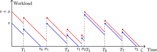
Notes. Blue (respectively, red) graph represents the workload process when the initial workload level is v (respectively, v + x). Each jump that occurs during the interval contributes x to the externality. Similarly, each jump that occurs during the interval contributes to the externality. In addition, each jump that occurs during the interval contributes to the externality. Finally, all jumps that occur after the coupling time ζ have no contribution to the externality, and hence the conclusion is that for the current realization we have that .
For every denote
In addition, define a right-continuous nondecreasing stochastic process (in x) as follows:
Then, for each ,
Theorem 1 implies that is a convex stochastic process. For more examples of convex stochastic processes that arise in different applications, see Jacobovic and Kella (2020).
For each , let S(y) be the number of jumps that has until
Notice that for every . Therefore, when replacing by in (21), this equation remains valid. Furthermore, the same technique that was applied in the proof of Proposition 1 can be used to show that is a compound Poisson process with rate λ and jump distribution . As a result, we obtain the following compact representation of the externalities process.
In the same probability space in which the model is defined, there is a compound Poisson process with rate λ and jump distribution such that
3.3. Decomposition 2
It is interesting to notice that equals the number of jumps of that cause an increase in the value of . Consider some arbitrary and denote
It is illustrated in Figure 2 that every jump of that causes an increase in the value of contributes x2 to the value of . This means that we can write
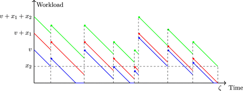
Notes. The green (respectively, red) graph describes a sample path of the workload process when a customer c with a service demand of (respectively, x1) arrives at time zero and sees a system with existing workload level v > 0. The blue graph describes a sample path of the workload of the same system once c reduces her service requirement to zero. The jumps of the graphs are coordinated. In fact, each jump is associated with an arrival of a customer and the size of the jump is the service demand of that customer. Observe that every jump on adds x2 to . In addition, the value of the green graph at ζ equals x2. Thus, a regenerative argument yields that is distributed as x2 multiplied by the number of jumps on plus an independent random variable that is distributed like .
Especially, because the workload process is strong Markov, the sum in the right-hand side is distributed as and is independent of (Figure 2).
Furthermore, assume that and is an i.i.d. sequence of random variables that are distributed uniformly on . In particular, assume that ξ, and are independent. In addition, for each we use the notation
This argument can be applied recursively to derive the following theorem. As illustrated in Section 4, it provides us with a systematic approach to compute the moments of the finite-dimensional distributions of .
Let and assume that and are such that:
is an infinite array of i.i.d. random variables such that is distributed according to .
is an infinite array of i.i.d. random variables that are distributed uniformly on .
are independent random variables such that and .
and are independent.
Then,
4. Moments of the Finite-Dimensional Distributions
This section concentrates on the evaluation of moments corresponding to the finite dimensional distributions of the externalities process . We first present the mean and variance and then the auto-covariance and auto-correlation, after which we proceed with higher moments.
4.1. Mean and Variance
Fix x > 0 and notice that an insertion of k = 1 into (28) yields
Thus, by an application of the formula of an expectation of a compound Poisson random variable, we directly obtain that
4.2. Auto-Covariance and Auto-Correlation
Fix some . Because the sums in the right-hand side of (29) are independent, we find
In addition,
As argued in the Introduction, in the situation of a customer arriving at time 0 with two tasks (of size x1 and x2, respectively), represents the total waiting time that could be saved by the other customers if the customer gave up on their second task but insisted on completing the first one. The auto-covariance (35) provides insight into the effect of the additional x2.
As a result, the auto-correlation function is given by
Surprisingly, the expression in (36) is invariant with respect to the service distribution and the arrival rate. At the same time, observe that is positive. In addition, the expression of actually shows that the externalities process is not wide sense stationary (see the definition in Yaglom (2004), p. 15).
In Section 7, we consider a setup in which v is a general nonnegative random variable, independent from the arrival process and service requirements. There, it is shown that in the more complex setup, the auto-correlation function depends on the arrival rate and service distribution unless v is a degenerate random variable.
4.3. Higher Moments
Higher moments (including joint moments) of may be derived via differentiation of the LST formula that is given in the next theorem. This is a tedious derivation that we decided to leave out. The result is particularly useful when analyzing a situation in which the customer arriving at time 0 has k tasks, having sizes .
Let and . In addition, define
Then, for any v > 0,
5. Crossing Times of
The process is nondecreasing such that , and as . Therefore, it is natural to study the crossing times of the process . Namely, fix some y > 0, and the corresponding crossing time is
In the remainder of this paper, we consider the special case v = 0 for which M = 0, and hence has a relatively tractable representation (but see Remark 5 for some reflections on the case v > 0). In fact, Theorem 2 yields that
It is well known that the mean of can be characterized via
Therefore, Wald’s identity may be applied to (42) to deduce that
The second moment of can be computed using a similar technique, thus also yielding . Hence, it is possible to compute the variance of x(y) via the formula
When v > 0, it makes sense to rely on a similar computation in which we condition and de-condition on M. In practice, we do not see how this computation leads to a tractable expression for the general case.
6. Gaussian Approximation of
The main result of this section concerns a Gaussian approximation for the externalities process. To provide an accurate statement of this result, the model that was described in Section 3 is characterized by the triplet . Fix and consider a sequence of models
In addition, for each , denote the externalities process that is associated with the nth model by . Also, let be the probability mass function of the number of customers who got service during a single busy period of a FCFS M/G/1 queue with an arrival rate λn and a service distribution . Correspondingly, for each , denote
6.1. Functional Central Limit Theorem
The main result of this section is stated in the next functional central limit theorem.
Define, for a fixed ,
A stochastic process
(51)such that is a standard Wiener process.A sequence (in ) of stochastic processes
(52)
In addition, assume that the next conditions hold:
(i) as .
(ii) There is such that for every .
(iii) as .
Then,
Observe that checking condition (iii) is not straightforward because it is phrased in terms of the moments of . The following proposition presents two sets of sufficient conditions that are considerably easier to verify. Broadly speaking, the proof of these sets of conditions being sufficient relies on the expressions appearing in the statement of Corollary 1.
The following two claims hold
The condition
Assume that condition (i) is satisfied. Thus, if
At the same time, observe that (56) is not necessary for (57) even under the assumption that condition (i) is satisfied.
The general idea of the proof of Theorem 4 is as follows. Condition (ii) allows us to apply Corollary 2, and hence, for each , there is a compensated compound Poisson process with rate and jump distribution such that
Then, the crucial part of the proof is to show that
An extensive account of heavy-traffic approximations of queueing systems can be found in Whitt (2002). Notably, heavy-traffic approximations have been developed for various functionals of the queueing process (such as the number of customers and the waiting time), but to the best of our knowledge, we are the first to do so for the externalities process. This means that, in the strict sense, we cannot compare our Theorem 4 with existing results. This being said, there is a vast literature on Gaussian approximations for sequences of compound Poisson processes, related to Theorem 5 (that is heavily relied on in our derivation of Theorem 4); we therefore include in Section 6.2 a comparison between Theorem 5 and related results.
We proceed by discussing an immediate implication of Theorem 4. To this end, fixing , recall that it is well-known result that
Hence, under the conditions of Theorem 4, we conclude the following convergence:
In fact, taking into account (32), the current analysis gives a new proof for (60) that is not based on stochastic calculus at all but only on approximation of a standard Wiener process by normalized compensated compound Poisson processes. Because (60) is known and the current proof is not simpler than the existing one, we mention this result in passing.
6.2. Gaussian Approximation to Compound Poisson Process
In this section, we discuss a general Gaussian approximation result for compound Poisson processes and relate it to existing results. As mentioned, it is used in the proof of Theorem 4, but may have broader applications.
6.2.1. Gaussian Approximation Result.
The following theorem, proven in Section 9.4, includes a statement about a Gaussian approximation of a general compound Poisson process. Possibly, this theorem may have other applications besides those that appear in the current work.
For each , let be a compensated compound Poisson process with rate and jump distribution such that
In addition, denote
and assume that both of the following conditions hold:
(I) as .
(II) as .
Then,
Intuitively speaking, condition (I) implies that the jumps become more frequent as , whereas condition (II) makes sure that the jump distribution should not become too “wild” as .
6.2.2. Comparison with the Existing Literature.
Let be a compensated-compound Poisson process with rate λ and a jump distribution with finite fourth moment. Denote the standard deviation of the jump distribution by γ. Then, Khoshnevisan (1993, corollary 3.7) states conditions under which the sequence (in n) of processes
Consider the setup of Theorem 5 with (i.e., ) and . Then, we get that , and hence in that sense, the setup of Theorem 5 is more general.
Theorem 5 guarantees weak convergence in a different topological space.
Khoshnevisan (1993, corollary 3.7) requires that the fourth moment of the jump distribution is finite, whereas Theorem 5 imposes no conditions on the fourth moment of Fn (for any ).
In Khoshnevisan (1993, corollary 3.7), we get that λn grows linearly in n that implies condition (I), but obviously condition (I) might be satisfied in other asymptotic regimes.
In Khoshnevisan (1993 corollary 3.7), we get that νn and σn remain fixed (in n), and hence, due to the linear growth of λn, condition (II) is satisfied. Once again, obviously it could be satisfied in other asymptotic regimes as well.
Another result (Pang and Zheng 2017, theorem 1.1) is about a weak convergence in equipped with the Skorohod topology of a sequence of modulated compound Poisson processes. When all the processes in this sequence are compound Poisson processes (i.e., when the modulating Markov chains in the background are all degenerate ones), then Pang and Zheng (2017, assumption 1) is reduced to
Linear growth of the sequence λn as
The sequences (in n) of the means and standard deviations of Fn should both converge to constants
We conclude that there is a strong resemblance between the comparison of Theorem 5 with Pang and Zheng (2017, theorem 1.1) and the comparison of Theorem 5 with Khoshnevisan (1993, corollary 3.7).
Another strand of literature regards the properties of a sequence of compound Poisson processes that weakly converges to a limiting process (Sarkar and Sen 2005, Lambert et al. 2013, Lambert and Simatos 2015). This literature predominantly focuses on necessary conditions for weak convergence of such sequences, whereas Theorem 5 presents sufficient conditions.
7. When v Is a Random Variable
In this part, we revisit some results of the previous sections in the situation that v is a nonnegative random variable that is independent from the arrival process and the service requirements of the customers. The motivation for this extension of the existing framework lies in the fact that if v has the stationary distribution of an M/G/1 queue with an arrival rate λ and a service distribution , then we recover the setup of Haviv and Ritov (1998). For simplicity of notation, denote the conditional expectation (respectively, covariance) given v by (respectively, ).
7.1. Expressions for Moments
To begin with, it is immediate that the decompositions of Section 3 remain true when the initial workload v is a general random variable. Similarly, Theorem 4 may be phrased in the extended setup. This is because for every bounded uniformly continuous functional f, we may apply the law of total expectation and then apply the dominated convergence theorem with Theorem 4 to deduce the needed result (Pollard 2012, corollary IV.9).
A similar approach may be applied to derive the moments of the externalities process. For example, for every ,
Furthermore, for every deduce that
Thus, the law of total covariance yields that
In particular, when and , the following variance is obtained:
Equations (69) and (70) imply that the correlation is invariant to the arrival rate and the service distribution if and only if (or equivalently, when v equals a constant with a probability of one).
For higher moments, it is possible to differentiate the LST formula, as given in the next corollary. Just like in Section 4, we do not include these computations here. The proof follows from conditioning and de-conditioning on v with the result of Theorem 3.
Let and . In addition, denote the LST of v by
7.2. Comparison with Existing Literature
Haviv and Ritov (1998) considered the special case when v is distributed according to the stationary distribution of the corresponding M/G/1 queue with an arrival rate λ and a service distribution . In this case, the expected value of v is given by
Observe that an insertion of these formulae into (66) provides exactly the same expression as in Haviv and Ritov (1998, equation (7)). Thus, in that sense, the formulae in this section may be considered as a natural generalization of this theorem, as in our framework v can have any distribution. Importantly, the proof in the current work stems from other considerations than those that appeared in the original proof of Haviv and Ritov (1998). Moreover, Corollary 3 might be applied for the special case of v that is distributed according to the stationary distribution of the corresponding M/G/1 system. This is a systematic approach to compute all externality moments in the model of Haviv and Ritov (1998).
8. Discussion and Open Problems
The main contributions of this work lie in the introduction of the notion of the externalities process and in the derivation of various of its properties in the case of an FCFS M/G/1 queue. The rest of this section includes a set of open problems, related to the research presented in this paper.
The current analysis is sensitive to the service discipline in that it is FCFS specific. Thus, it might be interesting to analyze the externalities process that corresponds to other service disciplines (e.g., preemptive ones) and examine the differences with respect to the results of the present paper. A particularly intriguing question concerns the characterization of the set of service disciplines for which the externalities process is convex.
One could think about the externalities processes of more complex queues, for example, G/G/1 and Mt/G/1. It is anticipated that in such cases the analysis is considerably more involved.
Consider the following natural multiserver version of the externalities process. Assume that there are k servers and a Poisson arrival process of customers, where the service demands of the customers constitute a sequence of i.i.d. k-dimensional nonnegative random vectors that are independent from the arrival process. This defines k coupled FCFS M/G/1 queues. Then, define a k-dimensional process such that its ith () coordinate is the externalities process that is associated with the ith queue. Also, in this setup, one would like to describe the externalities process. A specific natural question is: Are there nontrivial assumptions on the k-dimensional service distributions under which we get an asymptotic independence of the externalities processes?
The Lévy-driven queue, as analyzed in Dȩbicki and Mandjes (2015), forms a class of storage models that can be seen as a natural generalization of the classic FCFS M/G/1 queue. A first question is as follows: How should the externalities process be defined for such Lévy queues? In particular, it is interesting to analyze whether there is a definition for which the results of the current work may be generalized relying on the machinery developed for Lévy processes.
9. Proofs
9.1. Proofs for Section 2
9.1.1. Proof of Proposition 2.
Define a function
In particular, when x = 1, we get that . As a result, according to the Faá di Bruno’s formula, for each ,
Thus, observe that differentiating n times (at zero) for both sides of (9) with the general Leibniz rule yields
Notice that ηn appears in the right-hand side only in the term
This immediately yields the required recursive formula. □
9.1.2. Proof of Corollary 1.
Inserting n = 1 into (12) immediately yields that . In addition,
Thus, according to (12),
In a similar fashion, we get that
9.1.3. Proof of Proposition 3.
follows by differentiating both sides of (14) at zero. Now, consider some , then the general Leibniz rule and the Faá di Bruno’s formula (recall , defined in (74)) yield
9.2. Proofs for Section 3
The proofs of Corollary 2 and Theorem 2 follow directly from the material presented in Section 3. Thus, we are now providing only the proof of Theorem 1.
9.2.1. Proof of Theorem 1.
Observe that by definition of , for each and y > 0,
As a result, for every x > 0 we have that
With this identity at our disposal, the required result is a consequence of (18). □
9.3. Proofs of Section 4
9.3.1. Proof of Corollary 3.
With the notations that have been used in Theorem 2, observe that (28) can be rephrased as follows:
Thus, we obtain that
Given , the sequences are independent. As a consequence, the result follows by conditioning and de-conditioning on with an application of the LST formula of a compound Poisson distribution. □
9.4. Proofs of Section 6
Because the proof of Theorem 4 includes an application of Theorem 5, we start by providing the proof of Theorem 5.
9.4.1. Proof of Theorem 5.
The following well-known bound is useful in the proof of Theorem 5:
With this bound in hands, we prove convergence of the finite-dimensional distributions as stated in the next lemma. For the proof, it is convenient to denote
The conditions of Theorem 5 imply that for every and ,
To begin with, consider the special case d = 1 and assume that for each , Wn is a random variable which is distributed according to . Fix some and for each denote
In particular, (87) implies that for every ,
Thus, for a fixed and every , we have
The next stage is to extend this result for d > 1. To this end, for each , define d i.i.d. stochastic processes
Now, we are ready to prove the next lemma that is about validity of a tightness condition.
For every , there exist and such that
Fix some and take some . Notice that is a process with stationary increments, and has a continuous distribution function. Therefore, Lemma 1 yields that
Clearly, the probability in the right-hand side of (100) can be made sufficiently close to one by taking s and t, which are close enough to each other, and hence the result follows. □
Finally, for each has independent increments. Thus, using Lemmas 1 and 2, for each , Pollard (2012, theorem V.19) gives the required convergence on equipped with the uniform metric. Finally, to complete the proof of Theorem 5, it now suffices to apply Pollard (2012, theorem V.23). □
9.4.2. Proof of Theorem 4.
Let k > 0 and observe that condition (i), condition (ii), and condition (iii) allow us to apply Theorem 5 with the sequence to deduce that
Because the right-hand side converges to zero with a probability of one, deduce that the process
9.4.3. Proof of Proposition 4.
Inserting the expressions that appear in the statement of Corollary 1 yields that, for each ,
In addition, Jensen’s inequality yields that
Therefore, the assumption
Because of the first statement, to prove the second statement, it is enough to consider the case when as . Under the assumption
The authors thank Moshe Haviv for comments on an earlier version of the current work.
References
- (2021) Dynamic server assignment in multiclass queues with shifts, with applications to nurse staffing in emergency departments. Oper. Res. 69(6):1936–1959.Google Scholar
- (1969) The Single Server Queue (North-Holland Publishing Company, Amsterdam).Google Scholar
- (2015) Queues and Lévy Fluctuation Theory (Springer, Berlin).Google Scholar
- (2022) The important role of time limits when consumers choose their time in service. Management Sci. 68(9):6666–6686.Google Scholar
- (2001) Optimal pricing that coordinates queues with customer-chosen service requirements. Management Sci. 47(7):915–930.Google Scholar
- (2003) To Queue or Not to Queue: Equilibrium Behavior in Queueing Systems (Springer, Berlin).Google Scholar
- (2014) Regulating an M/G/1 queue when customers know their demand. Performance Evaluation 77:57–71.Google Scholar
- (2018a) Self-regulation of an unobservable queue. Management Sci. 64(5):2380–2389.Google Scholar
- (2018b) Social cost of deviation: New and old results on optimal customer behavior in queues. Queueing Models Service Management 1(2):31–58.Google Scholar
- (1998) Externalities, tangible externalities, and queue disciplines. Management Sci. 44(6):850–858.Google Scholar
- (2022) Optimal scheduling of proactive service with customer deterioration and improvement. Management Sci. 68(4):2533–2578.Google Scholar
- (2015) Control of patient flow in emergency departments, or multiclass queues with deadlines and feedback. Oper. Res. 63(4):892–908.Google Scholar
- (2022a) Internalization of externalities in queues with discretionary services. Queueing Systems 100(3–4):453–455.Google Scholar
- (2022b) Regulation of a single-server queue with customers who dynamically choose their service durations. Queueing Systems 101(3–4):245–290.Google Scholar
- (2020) Minimizing a stochastic convex function subject to stochastic constraints and some applications. Stochastic Processing Appl. 130(11):7004–7018.Google Scholar
- (1993) An embedding of compensated compound Poisson processes with applications to local times. Ann. Probability 3:340–361.Google Scholar
- (2015) Asymptotic behavior of local times of compound Poisson processes with drift in the infinite variance case. J. Theoretical Probability 28(1):41–91.Google Scholar
- (2013) Scaling limits via excursion theory: Interplay between Crump–Mode–Jagers branching processes and processor-sharing queues. Ann. Appl. Probability 23:2357–2381.Google Scholar
- (2022) Scheduling to differentiate service in a multiclass service system. Oper. Res. 70(1):527–544.Link, Google Scholar
- (2006) The distribution of the number of arrivals in a subinterval of a busy period of a single server queue. Queueing Systems 53:105–114.Google Scholar
- (2017) On the functional and local limit theorems for Markov modulated compound Poisson processes. Statist. Probability Lett. 129:131–140.Google Scholar
- (2012) Convergence of Stochastic Processes (Springer, Berlin).Google Scholar
- (2005) Weak convergence approach to compound Poisson risk processes perturbed by diffusion. Insurance Math. Econom. 36(3):421–432.Google Scholar
- (2002) Stochastic-Process Limits (Springer, Berlin).Google Scholar
- (2004) An Introduction to the Theory of Stationary Random Functions (Courier Corporation, Chelmsford, MA).Google Scholar