Optimization of Inventory and Capacity in Large-Scale Assembly Systems Using Extreme-Value Theory

1. Introduction

Delivery reliability is a key performance indicator for high-tech manufacturers, such as ASML, Philips, and Airbus. High-tech systems, such as wafer steppers, medical imaging equipment, and aircraft are produced by assembling thousands of components, each produced by highly skilled staff using specialized equipment. This production system facilitates modular design and testing, but it is also vulnerable: the shortage of a single component will result in delivery delays that cause customer grievances, a build-up of inventory of other components, and a severe reduction in turnover and cashflow. For example, in 2021, ASML was hit by material shortages in its supply chain, causing it to cut its revenue guidance (Denton 2021). Also, in other industries with higher demand volumes, for example, car manufacturing, many components are required to assemble the final product, and a single missing item can hinder production of the entire end-product. An example is the shutdown of complete manufacturing lines at several car manufacturers because of shortages of semiconductors (Ewing and Clark 2021).

Two complementary approaches may contribute to guaranteeing a reliable production system by reducing the risk of component shortages: excess component production capacity and inventory buffers. Production capacity and inventory buffers have a qualitatively different role in the mitigation of component shortages. Excess production capacity implies that the expected maximum number of components that can be produced per quarter exceeds the expected demand per quarter; for example, as a rule, production capacity may be 110% of expected demand. Inventory buffers are components that are produced in anticipation of demand; typically, such anticipative production continues until the inventory buffer reaches a target, for example, of six weeks of demand. Excess production capacity is always available, whereas inventory buffers are consumed when used to absorb production or demand fluctuations.

Joint optimization of excess component production capacity and component buffers is the ultimate goal because investments in excess component production capacity and component buffer inventories run into the hundreds of millions of euros (ASML Holding NV 2021). High-level investment plans for capacity and inventory may be devised for each product line (e.g., ASML’s TWINSCAN XT range or Philips’ Azurion 7 C range), depending on the role of the product line in the company’s portfolio and other considerations. Despite the strategic importance of these investments, there is a lack of quantitative methods for determining appropriate investments in capacity and inventory to achieve the desired level of delivery reliability. Indeed, despite decades of research in inventory management, the joint optimization of production capacity and inventory remains a considerable challenge (Bradley and Glynn 2002). Whereas the topic has increasingly been studied (see, e.g., Reed and Zhang 2017), the focus of analysis has been on problems with a single component. The much more common situation of assembling a system from many components has proved very challenging.

In this paper, we make a step toward overcoming this challenge. We propose a stylized model capturing key features of high-tech manufacturing that is based on interactions with high-tech manufacturers in the Netherlands and that yields new insights into the joint optimization of capacity and inventory for large-scale assembly systems. We focus on a single product line. Typically, a majority of the expensive components used in high-tech products are common to all products in a product line, being unique to that line, and we consider capacity and inventory optimization for those common components. Component shortages result in delays in the start of the assembly/integration process. Given the tight production planning that is common at high-tech manufacturers, such delays, in turn, result in costly delivery delays. Component production is capacitated and subject to random fluctuations. For example, the production capacity of components may be $\mu \pm \sigma$ items per quarter, and we assume a normal distribution for this per-period production capacity (e.g., Bradley and Glynn 2002, Wu and Chao 2014), which is the most natural assumption as the stochastic term represents the error around the mean. We adopt a continuous-time model, and we likewise assume that production capacity in every finite interval is linear with normally distributed white noise; that is, cumulative net production is a Brownian motion with drift $-\beta <0$ and variance ${\sigma }^2$ (cf. Bradley and Glynn 2002, Harrison 2013). We analyze the steady-state behavior of this system.

To analyze the overall production system, we consider a symmetric fork-join network of N queues driven by a common arrival process and having independent, identical service processes. Because of this common arrival process, total inventory per component, including backlogged items, is equal for all components. However, as a result of variations in the service times, the number of backlogged items may vary per component. We express the optimal component production capacity and inventory in this model in terms of the steady-state delay distribution of the slowest component, which has the form of a maximum of N all-time suprema of Brownian motions, and we subsequently focus on analyzing this delay distribution. In particular, in large-scale systems with many components/queues, one can expect that the maximum delay (which is due to stochasticity of demand and service processes) grows without bound as a function of the size of the system. To analyze and quantify this phenomenon, we derive new analytic results for the delays in this fork-join network as $N\to \infty$. To do so, we make a major assumption, which is that the randomness and cost characteristics of each of the N suppliers are identical, resulting in a symmetric system with identical net service capacities and base-stock levels. The symmetry we impose makes a mathematical treatment of our model within reach. Whereas this is a shortcoming of our work, it already reveals useful insights, and we complement our analytic results with simulation experiments for asymmetric systems.

1.1. Extreme Value Analysis

Original equipment manufacturers (OEMs) typically level the demand to smooth the production process. Accordingly, in our base model, we assume that demand is completely leveled, which corresponds to a fork-join queue with a deterministic arrival stream. Extremes for this network as $N\to \infty$ are obtained using extreme value theory (EVT), and based on those results, in Section 4, we derive easy-to-calculate expressions for capacity and inventory that are asymptotically optimal as the number of components grows large. We provide order bounds between the costs under optimal and approximate inventory and capacity. In particular, inspired by the literature on call centers (Gans et al. 2003, Borst et al. 2004, van Leeuwaarden et al. 2019), we distinguish three regimes that depend on the growth rates of cost parameters and are determined by the probability γ_N of not having enough inventory. Given that ${\gamma }_N\to \gamma$, we say that the regime is balanced if $\gamma \in (0,1)$. Furthermore, we are in the quality-driven regime if γ = 0 and in the efficiency-driven regime if γ = 1. For the base model, we establish asymptotic cost optimality in all three regimes. For the balanced, quality-driven, and efficiency-driven regimes, we have convergence rates of $1/(N \log N),{\gamma }_N/(N \log (N/{\gamma }_N))$, and $1/\log N$, respectively.

1.2. Demand Fluctuations

Other than the number of produced components being stochastic, despite efforts to level demand, typically, some demand variation remains. Thus, a natural choice is that the demand has, apart from a linear term, a white noise term as well, which is normally distributed. Therefore, in Section 5, we assume that the cumulative stochastic demand for systems is modeled by a Brownian motion with variance ${\sigma }_A^2$. (cf. Bradley and Glynn 2002 for a single-component manufacturing system). This implies that the demand over any finite time period is a normal variable, which is a standard assumption in literature (e.g., Klosterhalfen et al. 2014, Atan and Rousseau 2016). In high-tech manufacturing, normally distributed demand is a suitable assumption especially when considering longer time periods, but it is also a reasonable approximation for shorter periods. As a consequence of these demand variations, component delays become dependent because they face the same stochastic demands from system assembly. The question is now how this affects the maximum delay as the number of queues/components $N\to \infty$. Most of the work in extreme value theory has been done for independent random variables(cf. Resnick 1987, de Haan and Ferreira 2006), and suitable results from extreme value theory are absent for our setting, rendering the analysis of extremes in the dependent case challenging.

1.3. New Extreme Value Limit

Our answer to this challenge is somewhat surprising: in Theorem 5.1, we prove that the scaled maximum queue length converges to a normally distributed random variable as $N\to \infty$. In particular, if $Q_i(\infty ,\beta )$ is the invariant queue length at node i,

with X standard normal. An intuitive explanation of this result is the following. Using Lindley’s recursion, we can write the maximum queue length as a maximum of N suprema. By using subadditivity arguments, we can separate the independent and dependent parts; the independent part converges using standard extreme value results, whereas the dependent part satisfies a central limit theorem. To the best of our knowledge, we are the first who prove a result of this type. A consequence of this convergence result is that, with proper scaling of holding and backorder costs, the optimal inventory for stochastic demand converges to a scaled version of the quantile function of the normal distribution, whereas this quantile function also appears in the limit of the optimal capacity.

1.4. Numerical Experiments

In Section 5.3, numerical experiments show that we typically are most of the time 10% off the optimum (e.g., when N is in the range from 10 to 100); cf. Tables 5 and 6. Naturally, the difference goes to zero as $N\to \infty$; cf. Theorem 5.2. We give an improvement of this approximation by combining our results for deterministic and stochastic demand. Based on this approximation, we optimize the capacity and inventory decisions, and we test the quality of these approximations through numerical experiments. It turns out that these approximations perform well already when considering a limited number of components and are typically less than 2% off the optimum.

1.5. Limitations of Simulation

In Section 5.3, we explain the simulation procedure in the case of stochastic demand. We aim to approximate the maximum queue length of the all-time supremum of N dependent Brownian motions. Because the dependence structure between two all-time suprema of Brownian motions is complicated, we cannot resort to an easy simulation procedure, for example, by using copulas. We, namely, need to simulate discretized approximations of all of these N Brownian paths. Subsequently, we need to cut the Brownian path at some finite time point. We then record the largest observations of all of these paths. Subsequently, we compute the maximum of N of these records to obtain one observation of a maximum queue length. Afterward, we need to repeat this procedure to collect data. Finally, we use the collected data to compute empirical means and to estimate quantile functions. This means that the computation time grows with at least N, the size of the fork-join queue. Besides, in this simulation procedure, a lot of discretization and approximation steps are needed, which increase the error. Though the simulation results give a clear indication of the convergence rate of our limit theorem for small fork-join queueing networks, clearly the procedure is unworkable for a system with a number of servers of the order of thousands, which, as a matter of fact, shows the usefulness of the limit in Theorem 5.1 as an approximation.

1.6. Summary of Results

In this paper, we study an assembly system with N components, in which the demand and the number of produced components are deterministic with some random perturbation, which is assumed to be normally distributed. Thus, the total delay for one component in steady state can be modeled by the all-time supremum of a Brownian motion. We model the system as a fork-join queue. We then use results from EVT to estimate the longest queue, and we minimize the total costs in the system using this approximation (cf. Theorems 4.1, 5.1, and 5.2 for the most important results).

1.7. New Insights

This paper generates new insights in fork-join queues that lead to new analytical results for an important class of assembly systems. This paper is the first to consider simultaneous optimization of inventory and capacity in a multicomponent assembly system with dependent delays. Because of the dependencies in delays, evaluating such a system with fixed capacity and inventory is already a difficult problem. We provide several asymptotically optimal expressions for capacity and inventory that are either in closed form or can easily be computed numerically. Our results may help OEMs to optimally allocate budget to capacity and inventory to cost-efficiently ensure timely deliveries to their customers.

1.8. Overview

The remainder of this paper is organized as follows. In Section 2, we provide an overview of relevant literature. We introduce the general mathematical model in Section 3 and subsequently present the optimization problem in which we need to decide on capacity and inventory to minimize costs. We study the assembly system with deterministic demand in Section 4. We provide explicit expressions and approximations for optimal inventory and capacity. The stochastic demand case with solutions to the minimization problem and convergence results is studied in more detail in Section 5. A refinement of the approximations from Section 5 is provided in Section 6, in which we combine the lessons learned in Sections 4 and 5 to obtain better approximations for optimal capacity and inventory. In Section 7, we briefly touch upon the case of asymmetric systems and demonstrate that, even in these settings, our result for symmetric systems remain useful. We give a summary and conclusions in Section 8 and provide most of the proofs in Appendix A.

2. Literature Review

Simultaneous optimization of capacity and inventory is an important problem in supply chain management, but the literature on this topic is limited because of the complexity of the problem (Bradley and Glynn 2002). Considering the interaction between a manufacturer and a single supplier, Chaturvedi and Martínez-de Albéniz (2016) discuss the trade-off between inventory and capacity and how properly diversifying supply sources can reduce inventory and capacity investments. Sleptchenko et al. (2003) study simultaneous optimization of spare part inventory and repair capacity. In the last decade, simultaneous optimization of capacity and inventory in a single supplier–manufacturer relationship has been studied increasingly (e.g., Reed and Zhang 2017, Reddy and Kumar 2020). Reed and Zhang (2017) show that the square root staffing rule of Halfin and Whitt (1981) is a valuable tool in optimizing inventory and capacity in a multiserver make-to-stock queue. Altendorfer and Minner (2011) study simultaneous optimization of inventory and planned lead time, and Mayorga and Ahn (2011) study the joint optimization of inventory and temporarily available additional capacity. Our work differs fundamentally from these studies as we consider the assembly of multiple components that face the same (stochastic) demand.

In particular, we derive extreme value results for multicomponent assembly systems as the number of components grows large in order to obtain asymptotically optimal capacity and inventory decisions. We are not aware of related studies of extreme values for inventory and capacity optimization, but the approach is conceptually related to studies that apply asymptotic analysis to analyze inventory control problems, and we next review this literature. Such studies typically analyze inventory models that are inherently high dimensional; asymptotic analysis may be used to derive much simpler optimization problems that form an accurate approximation in some relevant asymptotic regime. This approach has led to major progress in the analysis of inventory problems, for example, for lost sales models (Goldberg et al. 2016, Xin and Goldberg 2016), dual sourcing (Xin and Goldberg 2018), and assembly-to-order systems (Reiman and Wang 2015, Doğru et al. 2017) in the presence of large lead times. Assemble-to-order systems with high-volume demand are studied by Plambeck (2008) and Plambeck and Ward (2008), whereas Zhang et al. (2020) study policies for managing perishable inventory when the market size grows large. A comprehensive overview of advances using asymptotic analysis can be found in Goldberg et al. (2021). Whereas conceptually related, our analysis differs substantially because a queueing model rather than a Markov decision process underlies our problem, and we aim to analyze extremes in the queueing model to optimize certain model parameters. In that sense, our work is related to Glasserman (1997), who provides approximations for setting base-stock levels in single-stage and multistage systems that are asymptotically exact as the target service level or the backorder penalty becomes large. For single-product lost sales inventory systems under periodic review, Huh et al. (2009) show that order-up-to policies are asymptotically optimal when the lost sales penalty is large compared with the holding cost. Bijvank et al. (2014) show the robustness of this result when using the optimal base-stock levels of the corresponding backorder system instead of those of the lost sales system. The asymptotic analysis in this paper is also influenced by related problems for queues with many servers inspired by agent staffing problems in call centers; we refer to Borst et al. (2004), Gans et al. (2003), and van Leeuwaarden et al. (2019) for background.

Brownian motion models are common in the literature on inventory control. Optimal control of inventory that can be described by a Brownian motion is described by (Harrison 2013, section 7), who provides optimality conditions for both discounted and average cost criteria. Closely related to our work is the Brownian motion model presented by (Bradley and Glynn 2002, section 3) to study the trade-off between capacity and inventory. They provide closed-form approximations to the optimal capacity and base-stock levels in a system with a single item. We consider an assembly system in which multiple components are merged into one end product. This is an essential difference because, in our model, inventory does not only buffer against uncertain demand, but a component may also need to be stored when other components are not yet available.

We note that our study focuses on the common components of a single high-tech system, which is a considerably simpler problem than general assemble-to-order problems (cf. Atan et al. 2017). Our focus enables us to obtain results for the key trade-off between capacity, inventory, and delivery reliability, sidestepping the difficulties of inventory control in multiproduct assemble-to-order systems with component commonality (see, e.g., Song 1998, Lu and Song 2005, Reiman and Wang 2015, Atan et al. 2017).

Literature concerning simultaneous optimization of capacity and inventory in single-sourced assembly (or assembly-to-order) systems with multiple components is limited. Zou et al. (2004) study how supply chain efficiency can be increased by synchronizing processing times and delivery quantities. Pan and So (2016) consider the simultaneous optimization of component prices and production quantities in a two-supplier setting in which one supplier has uncertainty in the yield. Our main contribution, compared with the work of Zou et al. (2004) and Pan and So (2016), is that we provide approximations of the optimal capacity and base-stock levels that only require two moments.

To analyze the problem at hand, we examine fork-join queueing networks with N servers for which the arrival and service streams are almost deterministic with a Brownian component. Our goal is to find and investigate the maximum queue length as N goes to infinity. The queue lengths are dependent random variables because of the joint interarrivals. Thus, our paper is related to the convergence of extreme values (maximum queue lengths) of dependent random variables. An overview of early results on extreme value theory for dependent random variables is given in Leadbetter et al. (1983). The authors provide conditions when the sequence of random variables may be treated as a sequence of independent random variables; this is the case when the covariance of random variables X_i and X_j decreases when i and j are further apart from each other. They also present a convergence result for the joint all-time suprema of a finite number of dependent stationary processes; they prove in theorem 11.2.3 that, under some assumptions, the joint all-time suprema of a finite number of dependent stationary processes are mutually independent. This is somewhat related to the problem that we study; however, we do not investigate stationary processes, and we only look at the largest of the N all-time suprema, in which $N\to \infty$.

We investigate the extreme values for a sequence of N Brownian motions. To be precise, we examine the joint all-time suprema of N dependent Brownian motions with a negative and linear drift term when N is large. A lot of work has been done on joint suprema of Brownian motions. For instance, Kou and Zhong (2016) give the solution of the Laplace transform of joint first passage times in terms of the solution of a partial differential equation, for which the Brownian motions are dependent. Dębicki et al. (2020) analyze the tail asymptotics of the all-time suprema of two dependent Brownian motions. The joint suprema of a finite number of Brownian motions are also studied; cf. Dębicki et al. (2015), in which the authors give tail asymptotics of the joint suprema of independent Gaussian processes over a finite time interval. These are just three examples, but the literature is rich with variations around assumptions on independence and dependence or around whether drift terms are linear, with joint suprema of two or more than two processes, with suprema over finite and infinite time intervals, and with extensions to other Gaussian processes. In this paper, we specifically examine the maximum of N all-time suprema of dependent Brownian motions. In this respect, the work of Brown and Resnick (1977) comes the closest to our work. In that paper, the authors study process convergence of the scaled maximum of N independent Brownian motions to a stationary limiting process whose marginals are Gumbel distributed. However, we add to this by considering the maximum of the all-time suprema of N dependent Brownian motions.

Our work also relates to the literature on fork-join queues. Specifically, we study asymptotic results for a fork-join queueing system with N servers. Most exact results on fork-join queues are limited to systems with two service stations; cf. Flatto and Hahn (1984), Wright (1992), Baccelli (1985) and Klein (1988). For fork-join queues with more than two servers, only approximations of performance measures are given; cf. Ko and Serfozo (2004), Baccelli and Makowski (1989) and Nelson and Tantawi (1988). Most of these papers focus on fork-join queueing systems in which the number of servers is finite, whereas we investigate a fork-join queue in which N goes to infinity. Furthermore, in these papers, the focus lies on steady-state distributions and other one-dimensional performance measures. Work on the heavy-traffic process limit has also been done. For example, Varma (1990) derives a heavy-traffic analysis for fork-join queues and shows weak convergence of several processes, such as the joint queue lengths in front of each server. Furthermore, Nguyen (1993) proves that various appearing limiting processes are in fact multidimensional reflected Brownian motions. Nguyen (1994) extends this result to a fork-join queue with multiple job types. Lu and Pang (2015, 2017a, b) study fork-join networks. In Lu and Pang (2015), they investigate a fork-join network in which each service station has multiple servers under nonexchangeable synchronization and operates in the quality-driven regime. They derive functional central limit theorems for the number of tasks waiting in the waiting buffers for synchronization and for the number of synchronized jobs. In Lu and Pang (2017a), they extend this analysis to a fork-join network with a fixed number of service stations, each having many servers, in which the system operates in the Halfin–Whitt regime. In Lu and Pang (2017b), the authors investigate these heavy-traffic limits for a fixed number of infinite-server stations, for which services are dependent and could be disrupted. Finally, we mention Atar et al. (2012), who investigate the control of a fork-join queue in heavy traffic by using feedback procedures.

3. Model and Preliminaries

The production system of OEMs such as ASML, Philips, or Airbus consists of roughly two stages: (1) component production and (2) assembly/integration of components. This setup is crucial to enable the modular design, production, and testing of components, and substantial value is added in both stages. For these reasons, system integration is only initiated after customers have committed to purchasing the system. We consider a manufacturing system in which a manufacturer assembles a final product from N common components, in which N is a large number, meaning that all components are required whenever a product is assembled. Each component is produced on a single production line that involves highly skilled staff and specialized equipment. In anticipation of uncertain demand, an inventory buffer is built up: production continues until a target inventory position is reached, after which production is switched off until the inventory position drops below this target. Such base-stock policies are widely used for modeling component inventories (e.g., Akçay and Xu 2004, Bollapragada et al. 2004, Karsten et al. 2012). Also, in a high-tech manufacturing environment, in which capacity mainly refers to people working in cleanrooms that can be at work or have a day off instead of expensive machines with high start-up costs, such policies are suitable. Despite these inventory buffers, random delays may occur in the production process for each of the components.

3.1. Model

We adopt a symmetric, continuous-time model and assume that production capacity in every finite time interval is normally distributed, meaning that cumulative production is a Brownian motion with drift. We then look at this system in equilibrium and find a trade-off between investing in the base-stock buffer and investing in capacity. To efficiently satisfy demand of the end product, which may either be deterministic or stochastic, we need to decide how much capacity to establish for each component and how many finished components to keep on inventory as a buffer. Even though it is costly to establish capacity and hold inventory, not being able to satisfy demand gives rise to backorder costs. Therefore, we need to find capacity and inventory levels that minimize total expected costs.

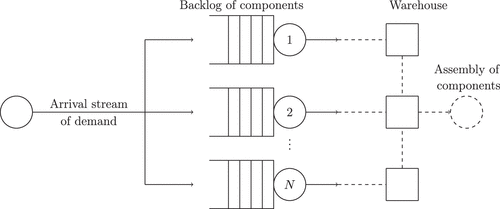
To analyze the cost-minimization problem, we model this assembly system by a fork-join network of N statistically identical but possibly correlated queues. Demand is represented by the common arrival process of jobs going to each server, and each server, with independent, identical service processes, represents production of a component. The backlog of each component is represented by a queue of jobs that have not been served yet. After completion of a job, the finished component is stored in a warehouse. As demand at each server is driven by a common arrival process, the total inventory of a component, including the number of backlogged components is equal for all components. However, as the service times vary, the division between the number of finished components and the number of backlogged components may vary per server. When all servers have a finished component in their warehouse, the end product can be assembled. This system is visualized in Figure 1.

3.2. Brownian Fork-Join Queue

We model queue lengths as reflected Brownian motions, following Harrison (1985) and Abate and Whitt (1987). Other papers using Brownian queues to analyze assembly systems are, for example, Plambeck (2008) and Plambeck and Ward (2008).

Definition 3.1.

For all $i\le N$, the service process at server i is governed by the Brownian motion $\{W_i(t),t\ge 0\}$ with standard deviation σ, and the arrival process is governed by the Brownian motion $\{W_A(t),t\ge 0\}$ with standard deviation σ_A. The queue length at server i at time t > 0 equals

$$Q_i(t,\beta )≔\underset{0<s<t}{\sup }((W_i(t)+W_A(t)-\beta t)-(W_i(s)+W_A(s)-\beta s)),$$(2)

with $Q_i(0,\beta )=0$. For $i,j\le N$ with $i\ne j$ the Brownian motions $\{W_i(t),t\ge 0\}$ and $\{W_j(t),t\ge 0\}$ are independent and identically distributed.

Formally, the Brownian motions $\{W_i(t),t\ge 0\}$ and $\{W_A(t),t\ge 0\}$ represent fluctuations in the service and arrival processes as they have zero mean. The controllable parameter β represents the excess capacity in each individual queue.

3.3. Base-Stock Level and Capacity

To buffer against uncertainties in the supply and demand processes, we introduce a base-stock level I_i for each component $i\le N$. We define ${\beta }_i>0$ as the net capacity for component i, that is, the difference between the production rate and arrival rate; in other words, β_i captures the capacity investment of server i. As mentioned before, we assume that, for all servers, the net capacity and the base-stock levels are the same; thus, ${\beta }_i={\beta }_j=\beta$ and $I_i=I_j=I$. The backlog $Q_i(t,\beta )$ represents the number of outstanding orders of component $i\le N$ at time t with $Q_i(t,\beta )$ given in Definition 3.1. If ${\sigma }_A^2>0,\hspace{0.17em}{(Q_i(t,\beta ))}_{i\le N}$ are dependent random variables.

3.4. Transient Inventory Levels and Backorders

We proceed by developing an expression for the total system costs, which requires expressions for the inventory and backorders. The inventory of component i consists of two parts: first, the excess supply that works as a buffer against uncertain demand and, second, the committed inventory that consists of items that are committed to realized demand but put aside because other components are not yet available. That is, the excess supply of component i is given by ${(I-Q_i(t,\beta ))}^{+}$. Moreover, the number of backorders for component i at time t is equal to ${(Q_i(t,\beta )-I)}^{+}$ because, for $Q_i(t,\beta )\le I$, the shortage is compensated by inventory I, and only the part of $Q_i(t,\beta )$ exceeding I represents actual backorders that cannot be satisfied. Because all components need to be available to assemble the final product, the number of backorders in the system is equal to the number of backorders of the component with the largest backlog and is, thus, given by ${\max }_{j\le N}{(Q_j(t,\beta )-I)}^{+}$. Therefore, the committed inventory of component i equals the number of backorders in the system minus its own backlog and can be expressed as ${\max }_{j\le N}{(Q_j(t,\beta )-I)}^{+}-{(Q_i(t,\beta )-I)}^{+}.$ The total inventory of component i at time t is, thus, given by

with $I_i(0)=I$. Observe that the total inventory $I_i(t)$ at time t is a function of the number of outstanding orders at time t. The reason why this is true is that the random variable $Q_i(t,\beta )$ does not depend on the total inventory because the servers always produce when there is an incoming task irrespective of whether there are items in stock or not. When there are items in stock, the product is immediately assembled, but servers work in order to reach the target inventory. When there are no items in stock, servers work to finish their component. Hence, whether a server works does not depend on the total inventory, but only on the demand and their own service speed. This means that the total inventory at time t is described as the function given in Equation (3). Thus, in order to know the total inventory on a certain time t, one should know the number of outstanding orders on that given time t when the dynamics of these outstanding orders are described as the dynamics of reflected Brownian motions until time t. Thus, this describes the dynamics of the system.

3.5. Steady-State Limit

Because the backlogs are modeled as reflected Brownian motions with negative drift, the backlogs have a steady-state limit. This limit extends to the largest backlog in the system and the total inventory of component i. We prove this in Lemma 3.1.

Lemma 3.1

(Steady State of Backlogs). Given $(Q_i(t,\beta ),i\le N)$ with $Q_i(t,\beta )$ defined in (2), we have that $(Q_i(t,\beta ),i\le N)\stackrel{d}{\to }(Q_i(\infty ,\beta ),i\le N)$ with

$$(Q_i(\infty ,\beta ),i\le N)\stackrel{d}{=}(\underset{s>0}{\sup }(W_i(s)+W_A(s)-\beta s),i\le N).$$(4)

In particular,

$$\underset{i\le N}{\max } Q_i(\infty ,\beta )\stackrel{d}{=}\underset{i\le N}{\max } \underset{s>0}{\sup }(W_i(s)+W_A(s)-\beta s).$$(5)

Proof.

The argument in one dimension is standard (see, e.g., section III.6 of Asmussen 2003); we extend it to our setting. Given t > 0, we can define Brownian motions $\{{\widehat{W}}_A(s),s\ge 0\}$ and $\{{\widehat{W}}_i(s),s\ge 0\}$ that satisfy ${\widehat{W}}_A(t-s)=W_A(t)-W_A(s)$ and ${\widehat{W}}_i(t-s)=W_i(t)-W_i(s)$. From this, it follows that, for fixed t > 0, we have that

$$\begin{array}{ll}(Q_i(t,\beta ),i\le N)\hfill & =(\underset{0\le s\le t}{\sup }({\widehat{W}}_i(s)+{\widehat{W}}_A(s)-\beta s),i\le N)\hfill \\ \hfill & \stackrel{d}{=}(\underset{0\le s\le t}{\sup }(W_i(s)+W_A(s)-\beta s),i\le N).\hfill \end{array}$$

Now, we obtain the lemma by letting $t\to \infty$, using monotone convergence. □

Combining this result with (3), we obtain an analogous result for the steady-state total inventory. In particular,

From now on, we write $Q_i(\beta )≔Q_i(\infty ,\beta )$.

3.6. Cost Function

We scale the cost of building net capacity to one and let $h^{(N)}$ and $b^{(N)}$ denote (inventory) holding costs and backorder costs, respectively, which may depend on N. Our goal is to minimize the expected total costs of the system in steady state.

Definition 3.2.

We define

$$C_N(I,\beta )≔\mathbb{E}\left[{\displaystyle \sum _{i\le N}\left[h^{(N)}\left(I-Q_i(\beta )+\underset{j\le N}{\max }{(Q_j(\beta )-I)}^{+}\right)\right]}+b^{(N)}\underset{j\le N}{\max }{(Q_j(\beta )-I)}^{+}\right],$$(6)

with the distribution of $Q_i(\beta )$ given in Equation (5).

Equation (6) simplifies to

$$C_N(I,\beta )=\mathbb{E}\left[N{h}^{(N)}(I-Q_i(\beta ))+(N{h}^{(N)}+b^{(N)}){\left(\underset{j\le N}{\max } Q_j(\beta )-I\right)}^{+}\right].$$

Then, the expected total costs in the system are equal to $C_N(I,\beta )+\beta N$, where the term βN reflects our normalization of unity net capacity costs per queue. If this term were removed, it would be optimal to choose $\beta =\infty$ and I = 0.

Because of the self-similarity of Brownian motion, we can write

$$\begin{array}{ll}\beta \underset{i\le N}{\max } \underset{s>0}{\sup }(W_A(s)+W_i(s)-\beta s)\hfill & =\beta \underset{i\le N}{\max } \underset{t>0}{\sup }\left(W_A\left(\frac{t}{{\beta }^2}\right)+W_i\left(\frac{t}{{\beta }^2}\right)-\beta \frac{t}{{\beta }^2}\right)\hfill \\ \hfill & \stackrel{d}{=}\underset{i\le N}{\max } \underset{t>0}{\sup }(W_A(t)+W_i(t)-t).\hfill \end{array}$$

This means that ${\max }_{i\le N}{Q}_i(\beta )\stackrel{d}{=}\frac{1}{\beta }{\max }_{i\le N}{Q}_i(1)$. Therefore, after rescaling the variable I, we can write

$$\underset{(I,\beta )}{\min }(C_N(I,\beta )+\beta N)=\underset{(I,\beta )}{\min }\left(\frac{1}{\beta }{C}_N(I\beta ,1)+\beta N\right)=\underset{(I,\beta )}{\min }\left(\frac{1}{\beta }{C}_N(I,1)+\beta N\right).$$(7)

In the last part of Equation (7), I has the interpretation of the base-stock level at which the net capacity β = 1. Therefore, from now on, the actual number of products on stock at time 0 equals $I/\beta$. Similarly, the actual unsatisfied demands of component i equals $Q_i(1)/\beta$, and we write $Q_i=Q_i(1)$. This allows us to write the cost function $F_N(I,\beta )$ to be optimized as given in Definition 3.3.

Definition 3.3.

We define

$$F_N(I,\beta )≔C_N(I,\beta )+\beta N=\frac{1}{\beta }{C}_N(I)+\beta N,$$(8)

with $C_N(I)≔C_N(I,1)$ and $C_N(I,\beta )$ given in Equation (6).

Our goal is to solve ${\min }_{(I,\beta )}{F}_N(I,\beta )$, focusing on the case in which N is large.

3.7. Preliminary Results

As we have defined the Brownian fork-join queue and the corresponding cost functions, we now state some general results that are valid regardless of whether ${\sigma }_A=0$ or ${\sigma }_A>0$. In the next lemma, we show that we can write ${\min }_{(I,\beta )}{F}_N(I,\beta )$ as two separate minimization problems.

Lemma 3.2.

Let ${(b^{(N)})}_{N\ge 1},{(h^{(N)})}_{N\ge 1}$ be sequences such that $h^{(N)}>0$ and $b^{(N)}>0$ for all N. Let $(I_N,{\beta }_N)$ minimize $F_N(I,\beta )$. Then, the optimal base-stock level I_N minimizes $C_N(I)$, and the optimal β_N minimizes $\frac{1}{\beta }{C}_N(I_N)+\beta N$. Furthermore, the function $C_N(I)$ is convex with respect to I, and the function $\frac{1}{\beta }{C}_N(I)+\beta N$ is convex with respect to β.

Using Lemma 3.2, we can characterize the optimal net capacity and base-stock level. In Lemma 3.3, we provide expressions for the optimal net capacity and costs in terms of the optimal base-stock level, which is given in Lemma 3.4.

Lemma 3.3.

Given $I_N^{*}={\text{arg min}}_I{C}_N(I)$, minimizing $F_N(I,\beta )$ with respect to β yields ${\beta }_N^{*}=\sqrt{\frac{C_N(I_N^{*})}{N}}$. Furthermore, the corresponding costs are $F_N(I_N^{*},{\beta }_N^{*})=2N{\beta }_N^{*}=2\sqrt{C_N(I_N^{*})N}$.

The optimal value of I can be expressed as a quantile of the distribution of ${\max }_{i\le N} Q_i$.

Lemma 3.4.

The optimal base-stock level $I_N^{*}$ is the unique solution of

$$\mathbb{P}\left(\underset{i\le N}{\max }{Q}_i\le I_N^{*}\right)=\frac{b^{(N)}}{N{h}^{(N)}+b^{(N)}}.$$

The main technical issue is that the distribution of this maximum is in general not very tractable, especially when N is large. The main theme of our work is to consider approximations of this distribution using extreme value theory to analyze their quality if N is large.

To explain our ideas, we mention the following first order approximation of ${\max }_{i\le N}{Q}_i$.

Lemma 3.5.

${\max }_{i\le N}{Q}_i$ satisfies the first order approximation

$$\frac{{\max }_{i\le N} Q_i}{\log N}\stackrel{L_1}{\to }\frac{{\sigma }^2}{2},$$

as $N\to \infty$.

The lemma easily follows from more refined results that are proven later on in this paper.

This first order approximation is valid regardless of whether ${\sigma }_A=0$ or ${\sigma }_A>0$. In the subsequent two sections, we consider more refined extreme value theory approximations covering both cases. It turns out that the second order behavior of the maximum is qualitatively different when σ_A becomes strictly positive. This has, in turn, an impact on the structure of the optimal solution of our cost minimization problem when N grows large.

To better understand this structure, we heuristically analyze the first order approximation of the cost-minimization problem and apply it to approximate $I_N^{*}$ and ${\beta }_N^{*}$. First, we use the approximation ${\max }_{i\le N}{Q}_i\approx \frac{{\sigma }^2}{2}\log N$ to write

The optimal value ${\overline{I}}_N$ for the associated first order minimization problem ${\min }_I{\overline{C}}_N(I)$ is given by ${\overline{I}}_N=\frac{{\sigma }^2}{2}\log N$ because $b^{(N)}>0$. Using this approximation, we see that $C_N({\overline{I}}_N)\approx {\overline{C}}_N({\overline{I}}_N)=(1+o(1))\frac{{\sigma }^2}{2}N{h}^{(N)} \log N,\hspace{0.17em}{\overline{\beta }}_N=\sqrt{{\overline{C}}_N({\overline{I}}_N)/N}=(1+o(1))\sqrt{\frac{{\sigma }^2}{2}{h}^{(N)} \log N}$, and $F_N({\overline{I}}_N,{\overline{\beta }}_N)\approx 2\sqrt{N}\sqrt{\frac{{\sigma }^2}{2}N{h}^{(N)} \log N}$. These results can be made rigorous, and the decision rule ${\overline{I}}_N$ can be shown to be asymptotically optimal, that is, that $F_N({\overline{I}}_N,{\overline{\beta }}_N)=F_N(I_N^{*},{\beta }_N^{*})(1+o(1))$. To prove this, we need to specify how the cost parameters $h^{(N)}$ and $b^{(N)}$ scale with N. For this, we consider three regimes. These regimes relate to the quantile $b^{(N)}/(N{h}^{(N)}+b^{(N)})$ of ${\max }_i{Q}_i$ at which $I_N^{*}$ attains its optimal solution. Assume that $b^{(N)}/(N{h}^{(N)}+b^{(N)})$ converges to a constant $1-\gamma$. We classify the three regimes in a similar way as is done in the analysis of large call centers; cf. Borst et al. (2004):

• We are in the balanced regime if $\gamma \in (0,1)$.

• If γ = 0, for large systems, the inventory is always sufficiently high to ensure that the manufacturer can assemble the end product. We call this the quality-driven regime.

• Finally, if γ = 1, inventories are much lower, and we call this the efficiency-driven regime.

When we are in the balanced or efficiency-driven regime we can prove how far the costs under the first order approximation are from the real optimal costs. This is established in Lemma 3.6.

Lemma 3.6.

Assume ${\gamma }_N=N{h}^{(N)}/(N{h}^{(N)}+b^{(N)})$ with ${\gamma }_N=\gamma \in (0,1)$ or ${\gamma }_N\stackrel{N\to \infty }{\to }1$. Then,

$$\frac{F_N(I_N^{*},{\beta }_N^{*})}{F_N({\overline{I}}_N,{\overline{\beta }}_N)}=1-o(1).$$

In the next two sections, we carry out a more elaborate program using more refined extreme value estimates of ${\max }_{i\le N}{Q}_i$. This analysis gives sharper order bounds than those given in Lemma 3.6. In particular, in the following sections, we consider the minimization in two distinct cases. First, in Section 4, we look at the case in which demand is assumed to be deterministic such that W_A = 0. Thereafter, in Section 5, we consider the stochastic demand case. In the former case, we utilize existing results in extreme value theory, whereas the latter case requires the development of a novel limit theorem. Furthermore, we use the result given in Corollary 3.1; this corollary shows how the ratio between the optimal costs and approximate costs can be represented when the approximate base-stock level and net capacity are solutions to a minimization problem as well. This corollary follows trivially from Lemma 3.3.

Corollary 3.1.

Assume we have a function ${\tilde{F}}_N(I,\beta ):(0,\infty )\times (0,\infty )\to \mathbb{R}$. Furthermore, assume that the function ${\tilde{F}}_N$ has the form

$${\tilde{F}}_N(I,\beta )=\frac{1}{\beta }{\tilde{C}}_N(I)+\beta N,$$

where ${\tilde{C}}_N$ is a positive function with domain $(0,\infty )$. Moreover, assume that the minimum value ${\tilde{F}}_N({\tilde{I}}_N,{\tilde{\beta }}_N)=2N{\tilde{\beta }}_N=2\sqrt{{\tilde{C}}_N({\tilde{I}}_N)N}$, where ${\tilde{I}}_N$ and ${\tilde{\beta }}_N$ are minimizers, so then,

$$\frac{F(I_N^{*},{\beta }_N^{*})}{F({\tilde{I}}_N,{\tilde{\beta }}_N)}=\frac{2\sqrt{C_N(I_N^{*})}\sqrt{{\tilde{C}}_N({\tilde{I}}_N)}}{C_N({\tilde{I}}_N)+{\tilde{C}}_N({\tilde{I}}_N)}.$$

4. The Basic Model: Deterministic Arrival Stream

In this section, we consider the case in which demand is deterministic. From this, it follows that all N queues are mutually independent.

4.1. Solution and Convergence of the Minimization Problem

We now analyze the minimization of the cost function described in Definition 3.3 for the special case with W_A = 0 representing deterministic demand. Although we can simplify the minimization problem significantly, by using the self-similarity of Brownian motions and by writing the minimization problem as two separate minimization problems, as shown in Lemma 3.2, the function F_N still has a difficult form because we have the expression ${\max }_{i\le N}{Q}_i$ in this function. In Lemma 4.1, we give the optimal base-stock level in order to minimize costs. We assume that the holding and backlog costs $h^{(N)}$ and $b^{(N)}$ are positive sequences, and we distinguish three cases. First of all, we consider the balanced regime ${\gamma }_N=N{h}^{(N)}/(N{h}^{(N)}+b^{(N)})=\gamma \in (0,1)$ for all n > 0. Second, we consider the quality-driven regime, in which ${\gamma }_N\stackrel{N\to \infty }{\to }0$. Finally, we investigate the efficiency-driven regime, in which ${\gamma }_N\stackrel{N\to \infty }{\to }1$. All proofs for this section can be found in Appendix A.2. We present numerical results for the three regimes in Section 4.2.

Lemma 4.1.

Let $Q_i={\sup }_{s>0}(W_i(s)-s)$ with $(W_i,1\le i\le N)$ independent Brownian motions with mean zero and variance ${\sigma }^2$. Let $h^{(N)}$ and $b^{(N)}$ be positive sequences. In order to minimize $F_N(I,\beta )$, the optimal base-stock level $I_N^{*}$ satisfies,

$$I_N^{*}=P_N^{-1}\left(1-{\gamma }_N\right)=\frac{{\sigma }^2}{2}\log \left(\frac{1}{1-{\left(1-{\gamma }_N\right)}^{\frac{1}{N}}}\right),$$(9)

with $P_N^{-1}$ the quantile function of $\mathbb{P}({\max }_{i\le N}{Q}_i<x)$ and ${\gamma }_N=N{h}^{(N)}/(N{h}^{(N)}+b^{(N)})$.

To get a better understanding of the limiting behavior of the solution to ${\min }_{(I,\beta )}{F}_N(I,\beta )$, we approximate the function F_N. Because $(Q_i,i\le N)$ are independent and exponentially distributed, we know by standard extreme value theory (cf. de Haan and Ferreira 2006) that $\frac{2}{{\sigma }^2}{\max }_{i\le N}{Q}_i-\log N\stackrel{d}{\to }G$ as $N\to \infty$ with $G\sim \text{Gumbel}$. Therefore, for N large, ${\max }_{i\le N}{Q}_i\stackrel{d}{\approx }\frac{{\sigma }^2}{2}G+\frac{{\sigma }^2}{2}\log N$. We get a new minimization problem when we replace ${\max }_{i\le N}{Q}_i$ with this approximation $\frac{{\sigma }^2}{2}G+\frac{{\sigma }^2}{2}\log N$. In Definition 4.1, we give the resulting function ${\widehat{F}}_N(I,\beta )$ that is to be minimized.

Definition 4.1.

$${\widehat{C}}_N(I)≔\mathbb{E}\left[N{h}^{(N)}\left(I-Q_i\right)+(N{h}^{(N)}+b^{(N)}){\left(\frac{{\sigma }^2}{2}G+\frac{{\sigma }^2}{2}\log N-I\right)}^{+}\right],$$(10)

and

$${\widehat{F}}_N(I,\beta )≔\frac{1}{\beta }{\widehat{C}}_N(I)+\beta N.$$(11)

In the remainder of this section, we investigate whether minimizing ${\widehat{F}}_N(I,\beta )$ results in costs that are close to those when we minimize $F_N(I,\beta )$. Note that we write $(I_N^{*},{\beta }_N^{*})$ for the minimizers of the cost function F_N defined in Definition 3.3, and we write $({\widehat{I}}_N,{\widehat{\beta }}_N)$ for the minimizers of the cost function ${\widehat{F}}_N$ defined in Definition 4.1. Throughout this paper, we indicate second order approximations by the $\wedge$-symbol.

In Proposition 4.1, we present the base-stock level that minimizes ${\widehat{F}}_N$. This base-stock level turns out to be a quantile of $\frac{{\sigma }^2}{2}G$ added to $\frac{{\sigma }^2}{2}\log N$.

Proposition 4.1

(Approximation). Minimizing ${\widehat{F}}_N(I,\beta )$ with $G\sim \text{Gumbel}$ gives solution $({\widehat{I}}_N,{\widehat{\beta }}_N,{\widehat{F}}_N({\widehat{I}}_N,{\widehat{\beta }}_N))$ with

$${\widehat{I}}_N=\frac{{\sigma }^2}{2}\log N-\frac{{\sigma }^2}{2}\log (-\log \left(1-{\gamma }_N\right)),$$(12)

and

$${\widehat{C}}_N({\widehat{I}}_N)=N{h}^{(N)}\left({\widehat{I}}_N-\frac{{\sigma }^2}{2}\right)+(N{h}^{(N)}+b^{(N)})\frac{{\sigma }^2}{2}\left({\displaystyle {\int }_{-\log \left(1-{\gamma }_N\right)}^{\infty }\frac{e^{-t}}{t}}dt+\mathrm{\Gamma }+\log (-\log \left(1-{\gamma }_N\right))\right),$$(13)

where $\mathrm{\Gamma }\approx 0.577$ is Euler’s constant and ${\gamma }_N=N{h}^{(N)}/(N{h}^{(N)}+b^{(N)})$.

Combining Equations (12) and (13) with the results in Lemma 3.3 gives the solution $({\widehat{I}}_N,{\widehat{\beta }}_N,{\widehat{F}}_N({\widehat{I}}_N,{\widehat{\beta }}_N))$.

We compare the costs under the optimal base-stock level and net capacity with the costs under the approximate base-stock level and net capacity. We distinguish the balanced, quality-driven, and efficiency-driven regimes.

By using the results from Lemmas A.1 and A.2 in Appendix A.2, we prove the order bounds in the balanced, quality-driven, and efficiency-driven regimes in Theorem 4.1. In the efficiency-driven regime, we impose the additional condition ${\gamma }_N<1-\exp (-N)$ needed to make sure that ${\widehat{I}}_N>0$. If we, namely, choose ${\gamma }_N>1-\exp (-N)$, we get that ${\widehat{I}}_N<0$, which is not feasible because ${\widehat{I}}_N$ has the physical meaning of the number of items that needs to be stored.

Theorem 4.1

(Order Bounds). Assume ${\gamma }_N=N{h}^{(N)}/(N{h}^{(N)}+b^{(N)})$ if ${\gamma }_N=\gamma \in (0,1)$ in the balanced regime. Then,

$$\frac{F_N(I_N^{*},{\beta }_N^{*})}{F_N({\widehat{I}}_N,{\widehat{\beta }}_N)}=1-O(1/(N \log N)),$$(14)

if ${\gamma }_N\stackrel{N\to \infty }{\to }0$ in the quality-driven regime. Then,

$$\frac{F_N(I_N^{*},{\beta }_N^{*})}{F_N({\widehat{I}}_N,{\widehat{\beta }}_N)}=1-O({\gamma }_N/(N \log (N/{\gamma }_N))),$$(15)

and if ${\gamma }_N\stackrel{N\to \infty }{\to }1$ and ${\gamma }_N<1-\exp (-N)$ in the efficiency-driven regime, then

$$\frac{F_N(I_N^{*},{\beta }_N^{*})}{F_N({\widehat{I}}_N,{\widehat{\beta }}_N)}=1-O(1/\log N).$$(16)

Using the order bounds given in Theorem 4.1, we can establish for the three different regimes how $F_N(I_N^{*},{\beta }_N^{*})$ scales with N as N becomes large.

Lemma 4.2.

Assume ${\gamma }_N=N{h}^{(N)}/(N{h}^{(N)}+b^{(N)})$ if ${\gamma }_N=\gamma \in (0,1)$ in the balanced regime. Then,

$$\begin{array}{ll}\hfill & F_N(I_N^{*},{\beta }_N^{*})\hfill \\ =2\sqrt{N}\sqrt{N{h}^{(N)}\frac{{\sigma }^2}{2}(\log N-\log (-\log (1-\gamma ))-1)+(N{h}^{(N)}+b^{(N)})\frac{{\sigma }^2}{2}\mathbb{E}\left[{(G+\log (-\log (1-\gamma )))}^{+}\right]}\hfill \\ +O(\sqrt{h^{(N)}}/\sqrt{\log N}),\hfill \end{array}$$(17)

if ${\gamma }_N\stackrel{N\to \infty }{\to }0$ in the quality-driven regime. Then,

$$\begin{array}{l}{F}_N(I_N^{*},{\beta }_N^{*})=2\sqrt{N}\sqrt{N{h}^{(N)}\frac{{\sigma }^2}{2}(\log (N/{\gamma }_N)-1)+(N{h}^{(N)}+b^{(N)})\frac{{\sigma }^2}{2}{\gamma }_N}\hfill \\ +O({\gamma }_N\sqrt{h^{(N)}}/\sqrt{\log (N/{\gamma }_N)}),\hfill \end{array}$$(18)

and if ${\gamma }_N\stackrel{N\to \infty }{\to }1$ and ${\gamma }_N<1-\exp (-N)$ in the efficiency-driven regime, then

$$F_N(I_N^{*},{\beta }_N^{*})=2\sqrt{N}\sqrt{N{h}^{(N)}\frac{{\sigma }^2}{2}\left(\log N-1\right)+b^{(N)}\frac{{\sigma }^2}{2}\log (-\log (1-{\gamma }_N))}+O(N\sqrt{h^{(N)}}/\sqrt{\log N}).$$(19)

The results given in Theorem 4.1 and Lemma 4.2 are obtained by using the properties stated in Online Lemmas A.1 and A.2. In Online Lemma A.1, we show that we can write a Gumbel distributed random variable that is on the same probability space as ${\max }_{i\le N}{Q}_i$. This gives us a very powerful result; namely, that ${\max }_{i\le N}{Q}_i$ and G_N are ordered and that their difference decreases as ${\max }_{i\le N}{Q}_i$ becomes large. Consequently, we obtain very sharp bounds on $|C_N(I_N^{*})-C_N({\widehat{I}}_N)|$ and $|{\widehat{C}}_N({\widehat{I}}_N)-C_N({\widehat{I}}_N)|$ in Online Lemma A.2, which leads to sharp results in Theorem 4.1 and Lemma 4.2.

4.2. Numerical Experiments

We now provide some numerical results to illustrate the solutions to the minimization problem and their characteristics discussed in Section 4.1. In all experiments, we let σ = 1 and let N vary from 10 to 1,000. The results for the balanced, quality-driven, and efficiency-driven regimes are given in Tables 1–3, respectively. We can observe that, in all regimes, the approximate solutions are close to the optimal solutions. Most importantly, already for small N, the fraction of the costs corresponding to the optimal solution over the costs corresponding to the approximate solution nearly equals one.

Table 1. Balanced Regime, $h^{(N)}=1,b^{(N)}=N$ Such That ${\gamma }_N=\frac{1}{2}$

Table 2. Quality-Driven Regime, $h^{(N)}=1,b^{(N)}=N^2$ Such That ${\gamma }_N=\frac{1}{1+N}$

Table 3. Efficiency-Driven Regime, $h^{(N)}=N,b^{(N)}=1$ Such That ${\gamma }_N=\frac{N^2}{N^2+1}$

5. Stochastic Demand

We now extend our framework to the case in which demand is stochastic. This means that stochasticity not only arises from the production process of the individual components, but also results from uncertain demands. Consequently, delays may no longer only be caused by low production of a specific component, but may also occur when there is a sudden peak in demand. Because all components need to be available to assemble the end product and satisfy demand, delays of the different components are now correlated. We use the same strategy when demand is stochastic as in the basic model with deterministic demand. However, we can no longer approximate the maximum queue length distribution with the Gumbel distribution. In Section 5.1, we show that, for N large, ${\max }_{i\le N}{Q}_i\approx \frac{{\sigma }^2}{2}\log N+\frac{\sigma {\sigma }_A}{\sqrt{2}}\sqrt{\log N}X$ with X a standard normal random variable. Using this approximation, we obtain a new minimization problem, in which we minimize ${\widehat{F}}_N^A(I,\beta )$ as given in Definition 5.1 with respect to I and β.

Definition 5.1.

$${\widehat{C}}_N^A(I)=\mathbb{E}\left[N{h}^{(N)}\left(I-Q_i\right)+(N{h}^{(N)}+b^{(N)}){\left(\frac{{\sigma }^2}{2}\log N+\frac{\sigma {\sigma }_A}{\sqrt{2}}\sqrt{\log N}X-I\right)}^{+}\right],$$

and

$${\widehat{F}}_N^A(I,\beta )=\frac{1}{\beta }{\widehat{C}}_N^A(I)+\beta N.$$

In Section 5.2, we elaborate on the solution and convergence of the minimization problem.

5.1. Extreme Value Limit

In this section, we focus on the maximum of N dependent random variables. In Theorem 5.1, we prove that a scaled version of ${\max }_{i\le N}{Q}_i(\beta )$ converges in distribution to a normally distributed random variable as N goes to infinity.

Theorem 5.1.

Let $(W_i,1\le i\le N)$ be independent Brownian motions with mean zero and variance ${\sigma }^2$ and W_A be a Brownian motion with mean zero and variance ${\sigma }_A^2$. Then,

$$\frac{{\max }_{i\le N} {\sup }_{s>0}(W_i(s)+W_A(s)-\beta s)-\frac{{\sigma }^2}{2\beta }\log N}{\sqrt{\log N}}\stackrel{d}{\to }\frac{\sigma {\sigma }_A}{\sqrt{2}\beta }X,$$(20)

with $X\sim \mathcal{N}(0,1)$. In other words, for all $x\in \mathbb{R}$,

$$\mathbb{P}(\frac{{\max }_{i\le N} {\sup }_{s>0}(W_i(s)+W_A(s)-\beta s)-\frac{{\sigma }^2}{2\beta }\log N}{\sqrt{\log N}}>x)\stackrel{N\to \infty }{\to }1-\mathrm{\Phi }\left(\frac{x\sqrt{2}\beta }{\sigma {\sigma }_A}\right),$$

with $\mathrm{\Phi }$ the cumulative distribution function of a standard normal random variable.

A heuristic explanation of the result in Theorem 5.1 is as follows: though $(Q_i,i\le N)$ are dependent random variables, because we are adding the same Brownian motion W_A, ${\max }_{i\le N}{W}_i(s)$ dominates more and more over W_A as N becomes larger. Consequently, W_A does not affect the time at which the supremum of ${\max }_{i\le N}{W}_i(s)+W_A(s)-\beta s$ is attained. Hence, for N large ${\max }_{i\le N}{Q}_i(\beta )\approx {\max }_{i\le N}{\sup }_{s>0}(W_i(s)-\beta s)+W_A(\tau )$ with τ the hitting time of the supremum of ${\max }_{i\le N}(W_i(s)-\beta s)$. Based on the theory on conditional expectations of Lévy processes, we know that the conditional expectation of the hitting time $\tau (x)$ to reach a point x is linear with x; to be precise, for n = 1, it is known that $\mathbb{E}[\tau (x)|\tau (x)<\infty ]=x/\beta$. Combining this with the fact that ${\max }_{i\le N} {\sup }_{s>0}(W_i(s)-\beta s)\sim \frac{{\sigma }^2}{2\beta }\log N$, we expect that the supremum of ${\max }_{i\le N}(W_i(s)-\beta s)$ is reached at $\tau \approx \frac{1}{\beta }·\frac{{\sigma }^2}{2\beta }\log N=\frac{{\sigma }^2}{2{\beta }^2}\log N$. Therefore, $W_A(\tau )\stackrel{d}{\approx }\frac{\sigma {\sigma }_A}{\sqrt{2}\beta }\sqrt{\log N}X$ with X standard normally distributed, which results in Equation (20).

The proof of Theorem 5.1 consists of four parts, which are stated in Lemmas 5.1–5.4 for which the proofs are provided in Appendix A.3. For a process X, we have for all t > 0 that

Furthermore, for every $0<t_1<t_2$,

We prove that these lower and upper bounds are tight for the process given in Theorem 5.1 for appropriately chosen $t,t_1,t_2$. More specifically, in Lemma 5.1, we prove the asymptotic behavior at the critical time $d\log N$, where $d=\frac{{\sigma }^2}{2{\beta }^2}$, resulting in the tight lower bound. We show that times before and after this critical time have no influence in Lemmas 5.2 and 5.3, respectively, leading up to Lemma 5.4 that shows the concentration around the critical time $d \log N$, proving a tight upper bound.

Lemma 5.1.

For $d=\frac{{\sigma }^2}{2{\beta }^2}$,

$$\frac{{\max }_{i\le N}(W_i(d \log N)+W_A(d \log N))-\beta d \log N-\frac{{\sigma }^2}{2\beta }\log N}{\sqrt{\log N}}\stackrel{d}{\to }\frac{\sigma {\sigma }_A}{\sqrt{2}\beta }X,$$(21)

with $X\sim \mathcal{N}(0,1)$ as $N\to \infty$.

Lemma 5.2.

For $d=\frac{{\sigma }^2}{2{\beta }^2}$ and $0<ϵ<d$ and for all x,

$$\mathbb{P}\left(\frac{{\max }_{i\le N} {\sup }_{0<s<(d-ϵ)\log N}(W_i(s)+W_A(s)-\beta s)-\frac{{\sigma }^2}{2\beta }\log N}{\sqrt{\log N}}\ge x\right)\stackrel{N\to \infty }{\to }0.$$(22)

Lemma 5.3.

For $d=\frac{{\sigma }^2}{2{\beta }^2}$ and all $ϵ>0$ and $x\in \mathbb{R}$,

$$\mathbb{P}\left(\frac{{\max }_{i\le N} {\sup }_{s\ge (d+ϵ)\log N}(W_i(s)+W_A(s)-\beta s)-\frac{{\sigma }^2}{2\beta }\log N}{\sqrt{\log N}}\ge x\right)\stackrel{N\to \infty }{\to }0.$$(23)

Lemma 5.4.

For $d=\frac{{\sigma }^2}{2{\beta }^2}$ and $ϵ>0$ and for all x,

$$\begin{array}{l}\underset{N\to \infty }{\text{lim sup}} \mathbb{P}\left(\frac{{\max }_{i\le N} {\sup }_{(d-ϵ)\log N\le s<(d+ϵ)\log N}\left(W_i(s)+W_A(s)-\beta s\right)-\frac{{\sigma }^2}{2\beta }\log N}{\sqrt{\log N}}\ge x\right)\hfill \\ \le \mathbb{P}\left({\sigma }_A\sqrt{\frac{{\sigma }^2}{2{\beta }^2}-ϵ}{X}_1+\sqrt{2ϵ}{\sigma }_A|X_2|>x\right),\hfill \end{array}$$(24)

with $X_1,X_2\sim \mathcal{N}(0,1)$ and independent.

In Appendix A.3, we show how these lemmas can be used to prove Theorem 5.1. In Lemma 5.5, we prove that convergence holds even in L₁ when X is chosen appropriately.

Lemma 5.5.

Define $X_N≔\frac{\sqrt{2}\beta }{\sigma {\sigma }_A}\frac{W_A(\frac{{\sigma }^2}{2{\beta }^2}\log N)}{\sqrt{\log N}}$. Then,

$$\mathbb{E}\left[\left|\frac{{\max }_{i\le N} {\sup }_{s>0}(W_i(s)+W_A(s)-\beta s)-\frac{{\sigma }^2}{2\beta }\log N}{\sqrt{\log N}}-\frac{\sigma {\sigma }_A}{\sqrt{2}\beta }{X}_N\right|\right]\stackrel{N\to \infty }{\to }0.$$

The proof of Lemma 5.5 is also given in Appendix A.3. In the next section, we apply Theorem 5.1 and Lemma 5.5 to solve and approximate the minimization problem. Specifically, Lemma 5.5 gives us an order bound between the optimal base-stock level and the approximate base-stock level.

5.2. Solution and Convergence of the Minimization Problem

We can use the convergence result proven in Theorem 5.1 to prove asymptotics of the minimization of the function F_N. Because $\frac{\sqrt{2}\beta }{\sigma {\sigma }_A}\frac{{\max }_{i\le N}{Q}_i(\beta )-\frac{{\sigma }^2}{2\beta }\log N}{\sqrt{\log N}}$ is a continuous random variable, we know that its quantile function converges to the quantile function of a standard normal random variable (cf. van der Vaart 1998, lemma 21.2). So we can use this to derive asymptotics of the minimization problem of F_N.

Using $P_N^A(z)$ as described in Definition 5.2, we can solve the minimization problem, which yields the optimal base-stock level and net capacity given in Lemma 5.6. The proofs concerning the solution and subsequent convergence results are provided in Appendix A.4.

Definition 5.2.

We define

$$P_N^A(z)=\mathbb{P}\left(\frac{\sqrt{2}}{\sigma {\sigma }_A}\frac{{\max }_{i\le N} Q_i-\frac{{\sigma }^2}{2}\log N}{\sqrt{\log N}}\le z\right).$$

Lemma 5.6.

Let ${(b^{(N)})}_{N\ge 1},{(h^{(N)})}_{N\ge 1}$ be sequences such that $h^{(N)}>0$ and $b^{(N)}>0$ for all N, and ${\gamma }_N=N{h}^{(N)}/(N{h}^{(N)}+b^{(N)})$. Let $({\beta }_N^A,I_N^A)$ minimize $F_N(I,\beta )$. Then,

$$I_N^A=\frac{{\sigma }^2}{2}\log N+\frac{\sigma {\sigma }_A}{\sqrt{2}}{P}_N^A{}^{-1}\left(1-{\gamma }_N\right)\sqrt{\log N}.$$(25)

When we are in the balanced regime, we can approximate the minimization problem given in Definition 5.1, using the convergence result in Theorem 5.1, and prove how far the approximate solution is from the optimal solution. This is done in Proposition 5.1 and Theorem 5.2. In Lemma 5.7, we show how the optimal costs scale with N when we are in the balanced regime. The proofs are given in Appendix A.4.

Proposition 5.1.

For ${(b^{(N)})}_{N\ge 1},{(h^{(N)})}_{N\ge 1}$ and ${\gamma }_N=N{h}^{(N)}/(N{h}^{(N)}+b^{(N)})$,

$${\widehat{I}}_N^A=\frac{{\sigma }^2}{2}\log N+\frac{\sigma {\sigma }_A}{\sqrt{2}}\sqrt{\log N}{\mathrm{\Phi }}^{-1}(1-{\gamma }_N),$$(26)

and

$${\widehat{C}}_N^A({\widehat{I}}_N^A)=N{h}^{(N)}\left(\frac{{\sigma }^2}{2}\log N-\frac{{\sigma }^2+{\sigma }_A^2}{2}\right)+(N{h}^{(N)}+b^{(N)})\frac{\sigma {\sigma }_A\sqrt{\log N}{e}^{-\frac{1}{2}{\mathrm{\Phi }}^{-1}{\left(1-{\gamma }_N\right)}^2}}{2\sqrt{\pi }}.$$(27)

Theorem 5.2

(Order Bound). Assume ${\gamma }_N=N{h}^{(N)}/(N{h}^{(N)}+b^{(N)})$ with ${\gamma }_N=\gamma \in (0,1)$. Then,

$$\left|\frac{F_N(I_N^A,{\beta }_N^A)}{F_N({\widehat{I}}_N^A,{\widehat{\beta }}_N^A)}-1\right|=o\left(\frac{1}{\sqrt{\log N}}\right).$$

Lemma 5.7

(Balanced Regime). Assume ${\gamma }_N=N{h}^{(N)}/(N{h}^{(N)}+b^{(N)})$ with ${\gamma }_N=\gamma \in (0,1)$. Then,

$$I_N^A=\frac{{\sigma }^2}{2}\log N+\frac{\sigma {\sigma }_A}{\sqrt{2}}\sqrt{\log N}{\mathrm{\Phi }}^{-1}\left(1-\gamma \right)+o(\sqrt{\log N}),$$(28)

and

$$F_N(I_N^A,{\beta }_N^A)=2\sqrt{N}\sqrt{{\widehat{C}}_N^A({\widehat{I}}_N^A)}+o(N\sqrt{h^{(N)}}).$$(29)

The result in Lemma 5.7 only holds for the balanced regime, so a natural question is what we can say about the efficiency- and quality-driven regimes. As is shown in Lemma 3.6, in the efficiency-driven regime, the first order approximation ${\overline{I}}_N=\frac{{\sigma }^2}{2}\log N$ gives that the ratio of the approximate costs and the optimal costs converge to one. Thus, we expect that the approximation given in (26) also satisfies this convergence result. In order to determine whether this approximation also satisfies the order bound given in Theorem 5.2, a further analysis is needed. The analysis we provide for the balanced regime heavily relies on van der Vaart (1998, lemma 21.2), which says that, if $Y_N\stackrel{d}{\to }Y$, then for $\gamma \in (0,1),\hspace{0.17em}{P}_{Y_N}^{-1}(\gamma )\stackrel{N\to \infty }{\to }{P}_Y^{-1}(\gamma )$. This gives us the convergence result (28) of the inventory in the balanced regime. In order to be able to prove a similar result for the efficiency-driven regime, we need an improvement of van der Vaart (1998, lemma 21.2), which also holds when ${\gamma }_N\stackrel{N\to \infty }{\to }1$.

However, for the quality-driven regime, this convergence result does not hold because we see in Lemma 4.2 that $I_N^A\approx \frac{{\sigma }^2}{2}\log (N/{\gamma }_N)$. In order to find a sharp order bound such as given in Theorem 5.2, we should resort to the analysis of tail asymptotics, which is beyond the scope of this study.

5.3. Numerical Experiments

In Section 5.2, we provided expressions to calculate the asymptotically optimal net capacity and base-stock level. The question remains how large the number of components has to be for these approximations to be of use. Therefore, we now examine the expected costs under both the optimal net capacity and base-stock level and under these asymptotic approximations. Because it is not straightforward to calculate $\mathbb{E}[{({\max }_{i\le N}{Q}_i-I)}^{+}]$ for dependent Q_i, to evaluate the cost function given in Definition 3.3, we resort to simulation. First, we explain the details of our simulation experiment, after which we discuss the numerical results.

In our simulation, we aim to determine the maximum delay over all components, so ${\max }_{i\le N}{Q}_i$. For this, we use the algorithm proposed by (Asmussen et al. 1995, section 4.5), who describe an exact algorithm for simulating a reflected Brownian motion at the grid points. At every grid point, we draw normal random variables with the required drift and variance for the supply and demand processes and update the maximum. We use a step size of 0.001 for the grid points. Because we cannot simulate over an infinite horizon, we have to determine when to terminate the simulation. The maximum value is expected to be attained at a time that is smaller than $\widehat{t}=\frac{{\sigma }^2+{\sigma }_A^2}{2}{\sum }_{j=1}^N\frac{1}{j}$. To simulate well beyond this point, we run the simulation until $t=2\widehat{t}$.

Using this method to simulate ${\max }_{i\le N}{Q}_i$, we can estimate $P_N^A{}^{-1}(1-{\gamma }_N)$ with $P_N^A(z)$ as described in Definition 5.2. To obtain a median-unbiased estimate of the quantile, we use the approach suggested by Zieliński (2009). For this, we sample ${\max }_{i\le N}{Q}_i$ 100 times and randomly choose between the observations $(1-{\gamma }_N)·100$ and $(1-{\gamma }_N)·100+1$ with weights depending on the value of the fractile. Our estimate is equal to the median over 100 iterations. Once we have our estimate of $P_N^A{}^{-1}(1-{\gamma }_N)$, we determine the value of the optimal base-stock level as given in Equation (25). Using the optimal base-stock level, we determine the optimal net capacity given in Lemma 3.3. Because this also requires the expectation of ${({\max }_{i\le N}{Q}_i-I)}^{+}$, we determine this value by taking the average based on 10,000 simulations.

Next, we compare the costs under our asymptotic approximations of the net capacity and base-stock level (provided in Proposition 5.1) to the costs under the optimal net capacity and base-stock level obtained from the simulation. We again sample ${({\max }_{i\le N}{Q}_i-I)}^{+}$ based on 10,000 new simulations and determine the costs of the different policies using cost function $F_N(I,\beta )$.

The procedure described is applicable for N in the order of hundreds; however, it is close to impossible to provide a fast simulation for N in the order of thousands. Hence, to give a useful approximation of the optimal capacity and base-stock level in these cases, we need to use the limit we derived in Theorem 5.1.

In order to assess the performance of the approximations and its sensitivity to various model parameters, we perform a full factorial experiment. In our experiment, we vary the number of components, demand variability, and backorder costs. The setup of the experiment is given in Table 4. We set $h^{(N)}=1$ and σ = 1 in all experiments. In total we have 24 instances. The results are given in Tables 5 and 6 for $b^{(N)}=N$ and $b^{(N)}=3N$, respectively.

Table 4. Parameter Settings for Experiments

There are several important observations to be made from Table 5. First of all, we can observe that, for n = 10, the difference in costs between the simulated optimal solution and the asymptotic solution is around 10% for most cases: the case n = 10 and ${\sigma }_A=1$ is an outlier, for which the difference is around 15%. As N increases to 50, the difference decreases. Furthermore, the difference becomes larger when σ increases. In the last column, we verify the convergence result from Theorem 5.2. We observe that the difference decreases as N increases and that increasing σ_A causes the difference to increase.

Table 5. Comparison of Costs Approximate Solution for $h^{(N)}=1,\hspace{0.17em}{b}^{(N)}=N$

When we consider the results for $b^{(N)}=3N$ given in Table 6, we observe that the difference between the asymptotic and optimal costs is considerably higher than for $b^{(N)}=N$. Especially for n = 10, the difference is around 15% of the optimum except for n = 10 and ${\sigma }_A=0.1$, for which the difference is around 20%. However, for a larger number of components, the difference is around 10% of the optimum. Interestingly, for the case ${\sigma }_A=1$, the difference between $b^{(N)}=N$ and $b^{(N)}=3N$ is relatively small.

Table 6. Comparison of Costs Approximate Solution for $h^{(N)}=1,\hspace{0.17em}{b}^{(N)}=3N$

Overall, in most of our experiments, the difference between the costs under the optimal base-stock level and net capacity and the costs under the approximations are around 10%. Furthermore, we can conclude that, for small variations in demand and low backorder costs, the asymptotic approach performs well in terms of costs already for a reasonable number of components. Also, the performance improves by increasing N. Finally, the performance of the approximations highly depends on the backorder costs relative to the holding costs.

6. Mixed-Behavior Approximations

The numerical results in Section 5.3 show that the approximations are in most of the cases around 10%–15% off the optimal value. In this section, we show how we can further improve the approximations.

Under deterministic and stochastic demand, the approximate problems are given in Definitions 4.1 and 5.1. If σ_A is small, then we know that, on the one hand,

because Q_i and Q_j are only slightly correlated. But, on the other hand,

Because the Gumbel term is missing here, this could be the reason that this approximation is not working well for small N. Thus, it could be beneficial to look at the combination of these two approximations. Then, we have

When we replace ${\max }_{i\le N}{Q}_i$ with Equation (30) in the minimization problem, we get

The optimal $I_N^M$ satisfies $\mathbb{P}\left(\frac{{\sigma }^2}{2}\log N+\frac{\sigma {\sigma }_A}{\sqrt{2}}\sqrt{\log N}X+\frac{{\sigma }^2}{2}G<I_N^M\right)=1-{\gamma }_N$. Thus,

Now, $I_N^M$ can be computed through standard numerical methods such as the bisection method. Furthermore, the optimal net capacity ${\beta }_N^M$ satisfies

The relevant expectations in this symbolic expression can be computed numerically; see Appendix A.5 for details.

6.1. Numerical Results Mixed-Behavior Approximations

Using the same simulation procedure as described in Section 5.3, we evaluate the performance of these adjusted approximations. The results for the cases of $h^{(N)}=1,\hspace{0.17em}{b}^{(N)}=N$ and $h^{(N)}=1,\hspace{0.17em}{b}^{(N)}=3N$ are given in Tables 7 and 8, respectively.

Table 7. Comparison of Costs Master Solution for $h^{(N)}=1,\hspace{0.17em}{b}^{(N)}=N$

Table 8. Comparison of Costs Master Solution for $h^{(N)}=1,\hspace{0.17em}{b}^{(N)}=3N$

From the simulation results, we can conclude that these adjusted approximations result in costs that are much closer to the optimal costs already for small N. When comparing the last two columns, in which the last column repeats the results from Section 5.3, we observe that the mixed-behavior approximations show better convergence also when σ_A is larger. Furthermore, when we saw in Section 5.3 that the cost difference increased considerably with the change in $b^{(N)}$, we now do see a slight increase, but the difference is still small for a larger value of $b^{(N)}$. Therefore, we can conclude that these mixed-behavior approximations perform well especially when demand variations are no more than 75% of the variations in component production even with a small number of components.

7. Analyzing Asymmetric Systems

This paper derives several new, analytical results for joint capacity and inventory optimization for large-scale, symmetric assembly systems. In this section, we provide an informal discussion of the application of such results in asymmetric settings.

For ease of exposition, consider a case in which different components have different holding costs. For other parameters, our assumptions remain in place. In practical settings, component prices might range from a few thousand to hundreds of thousands of euros. Companies seeking to apply advanced methods for optimizing capacity and inventory investments focus on the most expensive components: for inexpensive components, some coarse heuristics would suffice.

Suppose the company seeks to derive separate inventory buffer and capacity rules for two groups of components: expensive and very expensive components. This yields k = 2 groups of components. We seek to apply our results on extremes as the total number of components N in these two groups grows large; we keep k and the ratio of components in the two groups fixed. Also, because we seek to derive rules at the group level, it makes sense to assume symmetry within groups, that is, by averaging cost parameters within the groups. For example, consider the following: $N/2$ servers have a holding cost $h_1^{(N)}$ and $N/2$ servers have a holding cost $h_2^{(N)}$. Then, we need to minimize

This is over $(I_1,I_2,{\beta }_1,{\beta }_2)$. Obviously,

The cost function in Equation (33) can, therefore, be bounded from above by

Our analytical results enable us to minimize this upper bound; for instance, choosing ${\tilde{h}}_{1,2}^{(N)}=h_{1,2}^{(N)}$ and ${\tilde{b}}_{1,2}^{(N)}=\frac{N}{2}{h}_{2,1}^{(N)}+b^{(N)}$ yields

This is the sum of two functions that can be minimized using the exact solutions that we derived. In Table 9, we compare numerically the actual costs under the capacity and base-stock level that are obtained by minimizing this upper bound with the costs under the optimal capacity and base-stock level. In this table, the ratio indicates how many servers have a holding cost $h_1^{(N)}$ and how many servers have a holding cost $h_2^{(N)}$; the 1:1 ratio corresponds to the preceding example, whereas the 1:3 ratio can be treated similarly. The table demonstrates that our asymptotic results may be useful when optimizing asymmetric systems as well as symmetric systems.

Table 9. Comparison of Optimal Costs and Costs Under Upper Bound Heuristic, σ = 1, ${\sigma }_A=0$

8. Conclusions

In this study, we define a large-scale assembly system in which N components are assembled into a final product. We study an assembly system with linear demand and production, subject to some random noise. Thus, we impose the natural assumption that this noise is normally distributed. Hence, delays per component are written as an all-time supremum of a Brownian motion minus a drift term. We aimed to minimize the total costs in the system with respect to the inventory and net capacity per component. The costs in the system consist of inventory holding costs for each component and penalty costs for delays in assembly of the final product, which is equal to the delay of the slowest produced component. Before attempting to solve the minimization problem, we simplified the minimization problem, using the self-similarity property of a Brownian motion, into two separate minimization problems. We distinguish two cases: First of all, we covered the case of deterministic demand, resulting in all delays being independent. Second, we investigated the case in which demand is stochastic and, consequently, delays of the components are dependent.

For the deterministic demand scenario, we prove order bounds for three different regimes: balanced, quality driven, and efficiency driven. Additionally, we verify numerically that, already for a limited number of components, our approximations result in costs that are very close to the costs corresponding to the optimal solution. For the stochastic demand scenario, we develop a limit theorem that we use to obtain approximate solutions. We show numerically that, even though, theoretically, these approximations perform well, for practical situations, there is still room for improvement. However, this limit theorem is still necessary for systems with N of the order of thousands because it is close to impossible to simulate these systems quickly. Therefore, we provide additional approximations for a mixed-behavior regime, in which we use a combination of the approximations for the deterministic and stochastic demand scenarios. We demonstrate numerically that these approximations perform very well already for a practical number of components.

Future work could extend the model to a decentralized minimization problem, in which the components are not produced in-house by the manufacturer, but are sourced at outside suppliers that have their own objectives, which results in an asymptotic analysis of a game theoretical equilibrium; cf. Nair et al. (2016), Gopalakrishnan et al. (2016), and Kumar and Randhawa (2010). Additionally, we expect that we can extend the result in Theorem 5.1 to general Lévy processes. However, the cost minimization problem relies heavily on the self-similarity property of Brownian motions. Thus, to solve the minimization problem for Lévy processes, other techniques are needed.

References

- (1987) Transient behavior of regulated Brownian motion I: Starting at the origin. Adv. Appl. Probab. 19(3):560–598.Google Scholar
- (2004) Joint inventory replenishment and component allocation optimization in an assemble-to-order system. Management Sci. 50(1):99–116.Link, Google Scholar
- (2011) Simultaneous optimization of capacity and planned lead time in a two-stage production system with different customer due dates. Eur. J. Oper. Res. 213(1):134–146.Google Scholar
ASML Holding NV (2021) ASML annual report 2020. Accessed July 5, 2021, https://www.asml.com/en/investors/annual-report/2020.Google Scholar- (2003) Applied Probability and Queues, vol. 2 (Springer, New York).Google Scholar
- (1995) Discretization error in simulation of one-dimensional reflecting Brownian motion. Ann. Appl. Probab. 5(4):875–896.Google Scholar
- (2016) Inventory optimization for perishables subject to supply disruptions. Optim. Lett. 10(1):89–108.Google Scholar
- (2017) Assemble-to-order systems: A review. Eur. J. Oper. Res. 261(3):866–879.Google Scholar
- (2012) Control of fork-join networks in heavy traffic. 2012 50th Annual Allerton Conf. Comm., Control. Comput. (IEEE, Piscataway, NJ), 823–830.Google Scholar
- (1985) Two parallel queues created by arrivals with two demands: The M/G/2 symmetrical case. RR-0426, INRIA. inria-00076130.Google Scholar
- (1989) Queueing models for systems with synchronization constraints. Proc. IEEE 77(1):138–161.Google Scholar
- (2014) Robustness of order-up-to policies in lost-sales inventory systems. Oper. Res. 62(5):1040–1047.Link, Google Scholar
- (2004) Managing two-stage serial inventory systems under demand and supply uncertainty and customer service level requirements. IIE Trans. 36(1):73–85.Google Scholar
- (2004) Dimensioning large call centers. Oper. Res. 52(1):17–34.Link, Google Scholar
- (2002) Managing capacity and inventory jointly in manufacturing systems. Management Sci. 48(2):273–288.Link, Google Scholar
- (1977) Extreme values of independent stochastic processes. J. Appl. Probab. 14(4):732–739.Google Scholar
- (2016) Safety stock, excess capacity or diversification: Trade-offs under supply and demand uncertainty. Production Oper. Management 25(1):77–95.Google Scholar
- (2006) Extreme Value Theory: An Introduction (Springer Science & Business Media, New York).Google Scholar
- (2020) Exact asymptotics of component-wise extrema of two-dimensional Brownian motion. Extremes 23:569–602.Google Scholar
- (2015) Extremes of vector-valued Gaussian processes: Exact asymptotics. Stochastic Processes Appl. 125(11):4039–4065.Google Scholar
- (2021) ASML cuts guidance in the face of supply chain issues: The chip stock is falling. Accessed February 7, 2022, https://www.barrons.com/articles/asml-cuts-guidance-supply-chain-issues-51634728074.Google Scholar
- (2017) Assemble-to-order inventory management via stochastic programming: Chained BOMs and the M-system. Production Oper. Management 26(3):446–468.Google Scholar
- (2021) Lack of tiny parts disrupts auto factories worldwide. The New York Times Online (January 13), https://www.nytimes.com/2021/01/13/business/auto-factories-semiconductor-chips.html.Google Scholar
- (1984) Two parallel queues created by arrivals with two demands I. SIAM J. Appl. Math. 44(5):1041–1053.Google Scholar
- (2003) Telephone call centers: Tutorial, review, and research prospects. Manufacturing Service Oper. Management 5(2):79–141.Link, Google Scholar
- (1997) Bounds and asymptotics for planning critical safety stocks. Oper. Res. 45(2):244–257.Link, Google Scholar
- (2021) A survey of recent progress in the asymptotic analysis of inventory systems. Production Oper. Management 30(6):1718–1750.Google Scholar
- (2016) Asymptotic optimality of constant-order policies for lost sales inventory models with large lead times. Math. Oper. Res. 41(3):898–913.Link, Google Scholar
- (2016) Routing and staffing when servers are strategic. Oper. Res. 64(4):1033–1050.Link, Google Scholar
- (1981) Heavy-traffic limits for queues with many exponential servers. Oper. Res. 29(3):567–588.Link, Google Scholar
- (1985) Brownian Motion and Stochastic Flow Systems (Wiley, New York).Google Scholar
- (2013) Brownian Models of Performance and Control (Cambridge University Press, Cambridge, UK).Google Scholar
- (2009) Asymptotic optimality of order-up-to policies in lost sales inventory systems. Management Sci. 55(3):404–420.Link, Google Scholar
- (2012) Inventory pooling games for expensive, low-demand spare parts. Naval Res. Logist. 59(5):311–324.Google Scholar
- (1988) Fredholm integral equations in queueing analysis. Unpublished PhD thesis, Rijksuniversiteit Utrecht, Netherlands.Google Scholar
- (2014) Strategic safety stock placement in supply networks with static dual supply. Manufacturing Service Oper. Management 16(2):204–219.Link, Google Scholar
- (2004) Response times in M/M/s fork-join networks. Adv. Appl. Probab. 36(3):854–871.Google Scholar
- (2016) First-passage times of two-dimensional Brownian motion. Adv. Appl. Probab. 48(4):1045–1060.Google Scholar
- (2010) Exploiting market size in service systems. Manufacturing Service Oper. Management 12(3):511–526.Link, Google Scholar
- (1983) Extremes and Related Properties of Random Sequences and Processes (Springer Science & Business Media, New York).Google Scholar
- (2015) Gaussian limits for a fork-join network with nonexchangeable synchronization in heavy traffic. Math. Oper. Res. 41(2):560–595.Link, Google Scholar
- (2017a) Heavy-traffic limits for a fork-join network in the Halfin-Whitt regime. Stoch. Systems 6(2):519–600.Link, Google Scholar
- (2017b) Heavy-traffic limits for an infinite-server fork–join queueing system with dependent and disruptive services. Queueing Systems 85(1–2):67–115.Google Scholar
- (2005) Order-based cost optimization in assemble-to-order systems. Oper. Res. 53(1):151–169.Link, Google Scholar
- (2011) Joint management of capacity and inventory in make-to-stock production systems with multi-class demand. Eur. J. Oper. Res. 212(2):312–324.Google Scholar
- (2016) Provisioning of large-scale systems: The interplay between network effects and strategic behavior in the user base. Management Sci. 62(6):1830–1841.Link, Google Scholar
- (1988) Approximate analysis of fork/join synchronization in parallel queues. IEEE Trans. Comput. 37(6):739–743.Google Scholar
- (1993) Processing networks with parallel and sequential tasks: Heavy traffic analysis and Brownian limits. Ann. Appl. Probab. 3(1):28–55.Google Scholar
- (1994) The trouble with diversity: Fork-join networks with heterogeneous customer population. Ann. Appl. Probab. 4(1):1–25.Google Scholar
- (2016) Component procurement strategies in decentralized assembly systems under supply uncertainty. IIE Trans. 48(3):267–282.Google Scholar
- (2008) Asymptotically optimal control for an assemble-to-order system with capacitated component production and fixed transport costs. Oper. Res. 56(5):1158–1171.Link, Google Scholar
- (2008) Optimal control of a high-volume assemble-to-order system with maximum leadtime quotation and expediting. Queueing Systems 60(1):1–69.Google Scholar
- (2020) Capacity investment and inventory planning for a hybrid manufacturing-remanufacturing system in the circular economy. Internat. J. Production Res. 59(8):2450–2478.Google Scholar
- (2017) Managing capacity and inventory jointly for multi-server make-to-stock queues. Queueing Systems 86:61–94.Google Scholar
- (2015) Asymptotically optimal inventory control for assemble-to-order systems with identical lead times. Oper. Res. 63(3):716–732.Link, Google Scholar
- (1987) Extreme Values, Regular Variation and Point Processes (Springer, New York).Google Scholar
- (2003) Trade-off between inventory and repair capacity in spare part networks. J. Oper. Res. Soc. 54(3):263–272.Google Scholar
- (1998) On the order fill rate in a multi-item, base-stock inventory system. Oper. Res. 46(6):831–845.Link, Google Scholar
- (1998) Asymptotic Statistics, Cambridge Series in Statistical and Probabilistic Mathematics (Cambridge University Press, Cambridge, UK).Google Scholar
- (2019) Economies-of-scale in many-server queueing systems: Tutorial and partial review of the QED Halfin–Whitt heavy-traffic regime. SIAM Rev. 61(3):403–440.Google Scholar
- (1990) Heavy and light traffic approximations for queues with synchronization constraints. Unpublished PhD thesis, University of Maryland, College Park, MD.Google Scholar
- (1992) Two parallel processors with coupled inputs. Adv. Appl. Probab. 24(4):986–1007.Google Scholar
- (2014) Optimal control of a Brownian production/inventory system with average cost criterion. Math. Oper. Res. 39(1):163–189.Link, Google Scholar
- (2016) Optimality gap of constant-order policies decays exponentially in the lead time for lost sales models. Oper. Res. 64(6):1556–1565.Link, Google Scholar
- (2018) Asymptotic optimality of tailored base-surge policies in dual-sourcing inventory systems. Management Sci. 64(1):437–452.Link, Google Scholar
- (2020) Simple policies with provable bounds for managing perishable inventory. Production Oper. Management 29(11):2637–2650.Google Scholar
- (2009) Optimal nonparametric quantile estimators. Toward a general theory. A survey. Comm. Statist. Theory Methods 38(7):980–992.Google Scholar
- (2004) Channel coordination in an assembly system facing uncertain demand with synchronized processing time and delivery quantity. Internat. J. Production Res. 42(22):4673–4689.Google Scholar