Interpretable Prediction Rules for Congestion Risk in Intensive Care Units
Abstract
We study the problem of predicting congestion risk in intensive care units (ICUs). Congestion is associated with poor service experience, high costs, and poor health outcomes. By predicting future congestion, decision makers can initiate preventive measures, such as rescheduling activities or increasing short-term capacity, to mitigate the effects of congestion. To this end, we consider well-established queueing models of ICUs and define “high-risk states” as system states that are likely to lead to congestion in the near future. We strive to formulate rules for determining whether a given system state is high risk. We design the rules to be interpretable (informally, easy to understand) for their practical appeal to stakeholders. We show that for simple Markovian queueing systems, such as the queue with multiple patient classes, our rules take the form of linear and quadratic functions on the state space. For more general queueing systems, we employ methods from queueing theory, simulation, and machine learning (ML) to devise interpretable prediction rules, and we demonstrate their effectiveness through an extensive computational study, which includes a large-scale ICU model validated using data. Our study shows that congestion risk can be effectively and transparently predicted using linear ML models and interpretable features engineered from the queueing model representation of the system.
History: This paper has been accepted for the Service Science/Stochastic Systems Joint Special Issue.
Supplemental Material: The online appendix is available at https://doi.org/10.1287/stsy.2022.0018.
1. Introduction
Congestion poses a major operational challenge to many service systems. It negatively affects the service quality by prolonging users’ waiting times, which results in low user satisfaction (Anderson et al. 2007), and in some cases, such as in medical settings, it may even put patients at risk (Chalfin et al. 2007). By anticipating congestion, managers can prepare for periods of overcrowding. For example, increasing staffing levels, reducing service times, and diverting or postponing arriving users can all help to alleviate crowdedness if timely implemented (see, e.g., Green et al. 2006, Batt and Terwiesch 2012, Xu and Chan 2016). These measures, however, are costly and must therefore be carefully executed. Moreover, deciding when to trigger these measures requires having an accurate estimate of the system’s future congestion status, which is challenging as it depends not only on the current occupancy but also, on the system’s future dynamics (i.e., arrivals and departures).
Although predicting congestion is beneficial for many service systems, it is particularly important in the context of intensive care units (ICUs). The ICU is a specialized unit in hospitals that treats patients with severe or life-threatening illnesses and injuries. ICU overcrowding has been associated with a lower likelihood of ICU admission (Robert et al. 2012), poor patients’ outcomes (Kim et al. 2016), shorter length of stay (LOS) (Chan et al. 2012, Kc and Terwiesch 2012), and higher readmission risk and mortality (Robert et al. 2012), highlighting the importance of anticipating and preparing for high-occupancy periods. Prediction of congestion in ICUs is also challenging; patients admitted to the ICU are highly heterogeneous, with different diagnoses, complexities, and recovery times. Indeed, a general ICU may admit patients from surgical, emergency, and inpatient departments as well as transfer patients from other hospitals—all requesting ICU access at different rates and with highly heterogeneous care needs. These complexities hinder the ability to make accurate predictions about congestion, which on one hand, is quite common but on the other hand, is not constantly present. For example, during the period 2005–2007, the mean hourly ICU occupancy in the United States was 68.2% ± 21.3% (standard deviation), with significantly higher rates in academic hospitals (78.7% ± 15.9%) (Wunsch et al. 2013).
Motivated by the need to preemptively respond to crowdedness in ICUs, we consider well-established queueing models of ICUs and strive to predict congestion risk. Although significant research has been done on various related prediction problems, such as predicting patients’ LOS (e.g., Bertsimas et al. 2022 and references therein) or waiting times (e.g., Ibrahim 2018), we take a different approach and focus on predicting the risk of congestion in ICUs. That is, we predict whether an ICU is likely to reach a critically high occupancy level at a prespecified point in time in the near future. Kuntz et al. (2015) show that when hospitals reach a critical utilization level, they cross a tipping point, beyond which the quality of medical care is severely impacted. It is therefore of interest to recognize ahead of time whether a system is likely to reach such a tipping point in order to initiate proper interventions. Specifically, we consider the queueing model representation of an ICU (i.e., a collection of system states and transition probabilities) and refer to system states likely to lead to congestion (or high occupancy) in the short term as “high-risk” states. Our goal is to develop simple predictive rules that can be used by practitioners for deciding whether a given state is high risk or not. Such rules could inform various complex high-stakes decisions and trigger costly preventive actions to mitigate the risk of system congestion. This is in line with recent research showing the value of anticipative policies. For example, motivated by the study of emergency departments (EDs), Xu and Chan (2016) demonstrate that proactive admission control policies could potentially reduce waiting times by up to 15% without impacting the overall volume of patients treated; their policies rely on having an accurate prediction of the future system status. This is exactly our goal: to devise accurate predictions of the system’s future status in the context of ICUs. Further and motivated by the wide use of alert systems in hospital bed capacity management (e.g., Ahalt et al. 2018), we formulate the prediction task as a classification (i.e., predicting whether a state is high risk) rather than a regression problem (i.e., predicting the risk level). Like those systems, we are interested in distinguishing between a critical situation and a noncritical situation in order to trigger an alert.
Without a doubt, devising accurate predictions is crucial for users’ adoption, yet the interpretability of the predictions, or the lack thereof, has also been identified as a major barrier to adoption (Lehmann et al. 2022). This is particularly important for healthcare managers who value the ability to understand the contributing factors to a given prediction as they inform difficult resource allocation decisions (e.g., postponing surgery). Indeed, the “black-box” nature of algorithms (Maddox et al. 2019) and the potential amplification of human-induced bias (Obermeyer et al. 2019) have been identified as deterrents of adoption for clinical decision making, and interpretability has been recognized as a desirable property in the design of predictive models that inform the management of resources and control of patient flow (Bertsimas et al. 2022). Although there is no universally accepted definition for the notion of interpretability (which further depends on the domain of the prediction problem), in healthcare (e.g., MDCalc 2022), scoring systems (sparse linear models) and sparse logical models (e.g., decision trees) that make use of intuitive features have been extensively used for decades and are widely considered to be comprehensible to users coming from all backgrounds (Rudin et al. 2022). It is our goal to develop predictive models of this nature (as part of the literature review, in Section 2.3 we describe at a high level the current view of the machine learning (ML) research community on the topic of interpretability).
Our approach relies on the queueing model representation of ICUs and uses both theoretical analysis and numerical methods to identify high-risk states and derive interpretable predictive rules. These rules are simple conditions on the state of the system that when satisfied, indicate that the system is likely to become congested in the near future. Queueing systems have been widely employed to model the dynamics of general service settings and of interest to us, of ICUs (see, for example, Armony et al. 2015 and the references therein). Despite the rich literature on queueing theory, to the best of our knowledge, the formulation of this problem—prediction of congestion risk in queueing systems—has not been studied before.
Our paper’s main contributions are the following.
New problem formulation and solution approach. We formulate the problem of devising interpretable rules to predict high-risk states in terms of congestion in queueing models of ICUs. We develop a solution approach that integrates queueing theory, simulation, and machine learning methods to create interpretable predictive rules.
Accurate rules for predicting congestion in ICU models. For Markovian queueing models of ICUs (Kim et al. 1999, Van Dijk and Kortbeek 2009, Chan et al. 2016), we show that linear functions of the state information generate accurate predictions via theoretical and numerical analyses with a mean (median) error rate around 0.3% (0%). For non-Markovian queues (Marmor et al. 2013), we find that linear models based on engineered features that hold information about patients’ remaining length of stay (RLOS) can accurately predict congestion risk with a mean (median) error rate of around 2.3% (2.4%). Our feature-generating process is novel as it integrates simulation, clustering, and training of ML models, expanding prior ideas of using queueing features (Ang et al. 2016) to enhance prediction. Our resulting prediction rules are interpretable by design because of (1) the easy-to-understand sparse linear model and (2) the interpretable feature construction. For the latter, we devise summary features based on the patients’ remaining LOS before being discharged. Intuitively, the resulting prediction rules are simple linear functions of the counts of “short-stay” and “long-stay” patients in the system, where the “short-stay” and “long-stay” denotations are a generalization based on remaining LOS, which is meaningfully crafted.
Comparison with purely data-driven approaches and quantifying the benefit of incorporating queueing models for prediction. Implementing our model-based approach requires calibrating a queueing model using real data, creating interpretable features, and training an interpretable ML model using data generated from the queueing model (hereafter, we will refer to it as “our approach” for short). This is in contrast to data-driven approaches that apply ML algorithms directly to real data without using a queueing representation of the system. We numerically compare the two approaches and show that our approach can learn rules more accurately than purely data-driven approaches. Moreover, the model-based approach is also robust to small misspecifications of the queueing model: that is, when the fitted queueing model does not exactly capture the real system’s dynamics.
Organization. The rest of the work is organized as follows. Section 2 surveys the relevant literature. Section 3 introduces notation and the prediction problem formulation. Section 4 studies predictive rules in Markovian queueing models. In Section 5, we focus on non-Markovian queueing systems and present our framework to generate interpretable rules. We illustrate the approach for a large-scale non-Markovian ICU queueing model that was calibrated using hospital data and compare it against various natural benchmarks. Section 6 discusses practical considerations in applying our approach, and Section 7 concludes the work.
2. Literature Review
Our work is closely related to prediction in queueing systems and healthcare operations management, as well as emerging topics on interpretable machine learning.
2.1. Prediction in Queueing Systems
Prediction in queueing systems often focuses on anticipating future arrivals (e.g., Abate and Whitt 1987), length of stay (e.g., Bertsimas et al. 2022), and sojourn and waiting times (Ibrahim and Whitt 2011). The quantities of interest can be either short-term (e.g., the time-dependent moments of the probability distribution of a given workload metric) (e.g., Abate and Whitt 1987) or long-term (e.g., the steady-state queue length) (Fendick and Whitt 1989) performance metrics. Our work corresponds to a short-term prediction problem related to congestion that, to our knowledge, has not been studied before.
Common approaches used for forecasting are either based on stochastic analysis of queueing models (e.g., Ibrahim and Whitt 2011) or data driven (e.g., Whitt and Zhang 2017). The former is generally challenging for short-term prediction, and analyses seldom lead to compact expressions, particularly when models incorporate complex features, such as time-varying rates and users’ heterogeneity (see Whitt 1999, Ibrahim 2018). On the other hand, numerous works have substantiated that combining queueing models and data mining techniques leads to robust and accurate predictions (Senderovich et al. 2015, Ang et al. 2016, Yang et al. 2016). By deriving prediction rules using machine learning algorithms on model-generated data, we are able to take advantage of both the conceptual validity of model-based predictors (i.e., queueing dynamics) and the predictive power of data-driven methods. Moreover, the rules we derive are simple and interpretable, unlike ambiguous black-box prediction rules obtained from simulation.
2.2. Healthcare Operations Management
Healthcare facilities (e.g., hospitals units and clinics) are often modeled as queueing systems or networks (e.g., Kim et al. 2014, Armony et al. 2015). This paper contributes to the literature from a new angle by providing interpretable rules to identify occupancy levels that can lead to future congestion in ICUs with high probability.
The ICU, one of the most costly and crowded hospital units, has long been studied by operations management researchers (Denton 2013). The continuous-time Markovian loss queue is often used to model ICUs, as in Ridge et al. (1998) ( with priorities), Kim et al. (1999) ( with four classes of patients), and Shmueli et al. (2003) ( with optimal admission policy). However, analytical models for ICUs are still relatively few compared with models for other hospital units, such as the ED and operation room (OR). Xu and Chan (2016) demonstrate the benefit of incorporating predictions about future arrivals when admitting patients to the ED. They show that in comparison with reactive policies that admit patients based on current congestion, policies that use information about future congestion can significantly reduce delays while servicing the same number of patients. Denton (2013) suggests that ICU models should incorporate patient acuity and heterogeneity as well as its interactions with other adjacent units. ICU dynamics have also been studied empirically. For instance, Kim et al. (2016) find that high ICU congestion is associated with a lower likelihood of admission, and Long and Mathews (2018) identify a speedup effect in boarding from ICU to the exit wards when the ICU occupancy level is high and a slowdown effect when wards are full. To capture some of the ICU’s unique dynamics, researchers have refined traditional queueing models. Griffiths et al. (2006) develop an queueing model, where H stands for hyperexponential distribution that accounts for a highly variable length of stay. Van Dijk and Kortbeek (2009) study the transition between OR and ICU by modeling the OR-ICU system as a Markovian tandem queueing (MTQ) network. Using a large data set of ICU visits, Chan et al. (2016) estimate the effect of boarding delays from ED to ICU on the total length of stay. They incorporate such effects into an queueing model where the service time follows an exponential distribution with a mean that increases with the congestion level according to a growth function f. In our paper, we derive rules for the loss queue, the queue, and the Markovian tandem queue, all of which are motivated by the aforementioned ICU research. Moreover, we study a tandem ICU model validated from historical data (Marmor et al. 2013). This model incorporates various interesting features, such as time-varying arrivals, non-Markovian length of stay, and probabilistic routing.
Related closely to our work, Whitt and Zhang (2019) predict future daily arrivals and hourly occupancy levels based on observational data using a time series model. Although our work also aims to predict future system status, we differ in several aspects. First, our rules are learned from model-generated data instead of observational data. Second, our approach can incorporate additional information (e.g., classes of patients), whereas their predictive model only utilizes data about arrivals and departures. Lastly, we consider prediction rules that are not only highly accurate but also, interpretable.
2.3. Interpretable Machine Learning
Interpretability of predictive models refers to the ability of decision makers to understand and explain the mechanisms driving model predictions. Although ML algorithms are commonly used for discovering patterns in data, the employed models often operate as black boxes (Chen et al. 2017). This could be problematic in applications where knowing why a model makes a certain prediction is critical (e.g., in assessing credit risk Baesens et al. 2003 or crime recidivism Zeng et al. 2017).
Interpretability is critical for healthcare applications because practitioners must be able to explain and clinically justify their actions (e.g., using decision trees) (see Lin et al. 2020 and the references therein). In addition, the discovery of important associations from an interpretable model can help providers make faster decisions based on simple and easy-to-explain rules (e.g., if-then rules) (Letham et al. 2015). An alternative to training interpretable models from data, which gained popularity recently, is applying algorithms that aim to explain the predictions of black-box models. Examples include methods such as Local Interpretable Model-agnostic Explanations (Ribeiro et al. 2016). However, there is an ongoing debate about the effectiveness and trustworthiness of such methods (Rudin 2019, Rudin and Shaposhnik 2023).
Although the majority of the work related to interpretable ML is applied to real-world data, a recent stream of work focuses on interpretable decision making rooted in stochastic models. Ciocan and Mišić (2022) study optimal stopping policies in stochastic systems. They formulate near-optimal policies as a tree, which is learned using simulated trajectories of the stochastic system. Similarly, Grand-Clément et al. (2021) propose a novel algorithm to compute interpretable tree policies for finite-horizon Markov devision process and demonstrate its value through a case study of ventilator allocations for coronavirus disease 2019 patients. Bravo and Shaposhnik (2020) use interpretable ML to extract insights from optimal solutions to optimization problems. Our work also contributes to this area; we focus on mining structural properties of stochastic models. However, different from previous work, we explore the application of ML to discover congestion-related patterns in queueing models. This is an effort to deduce interpretable and easy-to-use rules for managing congestion in healthcare, as well as in other service systems.
3. Problem Formulation
Consider a general queueing model of an ICU that is operating according to an arbitrary service discipline, with m patient classes of distinct arrival processes and service times. Denote by the possibly infinite collection of system states that may be encountered throughout the system’s evolution. We denote as the random state of the system at time , which may, for example, hold information about current patients, their arrival times, delays, elapsed processing times, the current time, etc. The state shall incorporate all the past information that is relevant for future system evolution.
Let or Lt for short denote the number of patients in the system at a particular state . We say that the system is congested when the number of patients in the system is greater than or equal to g (e.g., the value of g could be the number of used beds equivalent to a critical level of utilization in a ward or the number of nurses on the shift multiplied by the unit-specific nurse-to-patient ratio). We define a high-risk state as a state that leads to congestion with a sufficiently large probability, which is greater than α, at a certain future time . The value of is a look-ahead period that captures the lead time for intervention (e.g., minimal time for staff or patient rescheduling). The function is referred to as the congestion risk function, which quantifies the probability that the ICU becomes congested τ units of time into the future, namely
Using the congestion risk function , the sets of high- and low-risk states can be defined as
We define the true classifier (or equivalently, prediction rule) that discriminates between the two classes; for each state if , and otherwise.
The true classifier f may be difficult to derive analytically, and therefore, our goal is to find an approximate classifier that satisfies the following properties.
(Accuracy) according to some distance or cost metric.
(Interpretability) , where is a class of interpretable ML models (hypothesis class): that is, models that are easy to understand and apply by decision makers. Interpretability is often measured by sparsity (number of terms in a linear model and number of leaves in decision trees).
As discussed in Section 1, sparse linear models and decision trees that use meaningful features whose calculation can be explained are generally considered to be interpretable (Rudin et al. 2022).
3.1. Computational Approach for Deriving Rules from Queueing Models
For convenience, we normalize the time observing to time 0 and predict . As we shall see, deriving analytically is a nontrivial task as it requires estimating the distribution of the number of patients in the system at time . The latter depends on many factors, such as the arrival process, the service discipline, and the time from service commencement in an intricate way. Indeed, even in simple queueing systems, the analytical derivation is intractable (see Section 4.1.2). Combining queueing theory, simulation, and ML, we alternatively propose a numerical framework to study congestion in general queueing systems. Similarly to the Monte Carlo simulation approach in value at risk (VaR)1 estimation where historical returns are assumed to be governed by an underlying data-generating process (Linsmeier and Pearson 2000), we study the prediction problem by using the queueing model representation of the real system as the data-generating process. Thus, starting from a queueing representation of the system of interest, Figure 1 illustrates our overall framework, which consists of the following steps.
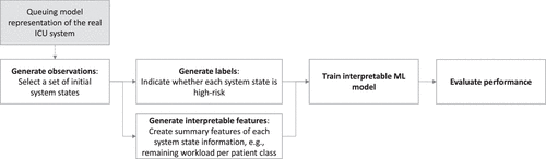
Generate Observations. We sample a large number of initial states from the queueing system. All states can be included for learning if the state space is finite. Otherwise, one could perform sampling to collect representative states. The state shall incorporate all the past information that is relevant for future system evolution. For example, for an loss queue, the state is formulated by counting the number of patients from each class currently in the ICU.
Generate Labels. For each state , we estimate its risk label according to the queueing dynamics. For example, for general queues, one can simulate multiple sample paths starting from the initial state and evaluate the probability of future congestion based on the sample average.
Generate Interpretable Features. Although the system state summarizes all the relevant information, feature engineering is performed to create summary features and improve the quality and interpretability of the prediction model. We denote the set of features by .
Train Interpretable ML Model. A data matrix can now be constructed, where each observation represents one state , its features , and the corresponding risk label . Following standard evaluation methods, we split the observations into two sets: training and test sets. The train data set is used to learn an interpretable ML model, and the test set is used to evaluate the performance and generalizability of the predictive model.
Evaluate Performance. We evaluate performance using standard metrics, such as accuracy, error rate, false-positive rate (FPR), and false-negative rate (FNR), and use 10-fold cross-validation for hyperparameter tuning.
The key challenge will be to develop effective features that permit accurate and interpretable ML models. In the rest of the paper, we study increasingly more complex queueing models of ICUs to provide theoretical and empirical justifications for our choices of features and ML models and demonstrate their effectiveness in predicting congestion risk.
4. Deriving Rules for Markovian Models
In this section, we show that using linear predictive models that use patient counts as features is effective for predicting congestion risk in Markovian models. To develop intuition, we first consider the canonical queueing systems and and summarize our analytical findings in Section 4.1. In Section 4.2, we apply our computational framework described in Section 3.1 to general Markovian queueing systems that are commonly used to model ICUs.
4.1. Insights from Analytical Solutions
To aid reading, we only present here the key results and defer the analysis to Online Appendices A () and B ().
4.1.1. Queue with m Patient Classes (in Short, ).
The model is well studied in the queueing literature (Guillemin and Simonian 1995, Knessl and Yang 2001), and although simplistic, we use it as a starting point to gain intuition about how queueing dynamics impact congestion risk.
Let μi and λi, respectively, denote the service and arrival rates of class i patients. We assume, without loss of generality, that and refer to patients with smaller values of μi as long-stay patients and to patients with larger values of μi as short-stay patients. We assume that service and interarrival times are independent among patients. Using the memorylessness property, the system state can be written as , where ni is the number of class i patients in the system. The true classifier is written as We compute the distribution of as the convolution of binomial and Poisson distributions (see Lemma EC.1 in Online Appendix A). Then, approximating by a normal distribution, we derive an approximate classifier that is quadratic in . Namely,
Interestingly, we observe that the decision boundary of the classifier is often approximately linear in . We formalize this property in the following lemma. Let the decision boundary be the set of points satisfying
Let z be an arbitrary point on the decision boundary of : that is, . Suppose further that for all such z, for some C > 1. Then, for all i, , we have
Because for any i, defines an implicit function of provides crucial information about its functional form. Intuitively, Lemma 1 implies that when the decision boundary crosses states with a sufficiently large number of patients, the normal approximation is more accurate, and the decision boundary becomes linear. To see this, note that large values of z allow C to be chosen as a large value, resulting in . The partial derivatives (for every pair of patient classes i and j) become constant, implying that the decision boundary is linear around z (the Taylor expansion of xi is ). To develop further intuition on Lemma 1, consider a few simple cases.
Case 1. . This recovers the straightforward situation where if the system has at least g patients at time 0; then, the system is obviously crowded when . In this case, . Thus, by Equation (1), for all i, j, and z, . In the extreme case when , the decision boundary is described by the function for some constant a, and thus, it is a linear function. Moreover, from the definition of , when τ = 0, it follows that pi = 1, qi = 0, and Λ = 0; thus, . Namely, the decision boundary is exactly .
Case 2. All service rates μi are equal. In this case, all pi’s are equal, and using Equation (1), it follows that for all i, j, and z. Thus, the decision boundary is a hyperplane (i.e., (for some constant b)).
Case 3. . In this case, . We can choose C to be arbitrarily large, so for all i, j, and z. Therefore, the decision boundary is again a hyperplane (i.e., for some constant c).
Although congestion may not be a major concern in a system with an infinite number of servers, such a system is often used as a first-order approximation of complex systems with the goal of gaining preliminary insights on their performance (De Bruin et al. 2007). Its analysis reveals a simple structure whereby the prediction rule can be approximated by quadratic and even linear functions of the number of patients from each class, which is interpretable, accurate, and practically appealing.
4.1.2. Queue with One Patient Class.
A more accurate model of ICUs accounts for their finite capacity. We consider capacitated Markovian systems, starting with a loss queue with a single patient class. Similar to the queue, the state Nt counts the patients in the unit at time t, and we note that it is a scalar (instead of a vector) and exactly equal to the occupancy of the unit. That is, . We show that the congestion risk is nondecreasing in N0.
( Monotonicity). For any state and integer , we have that
Proposition 1 guarantees the intuitive behavior that the congestion risk is nondecreasing in the initial number of patients in the system. To prove this, we derive the τ-period transient probability matrix (see pp. 167–168 in Tijms 2003). For any continuous-time Markov chain, the transient probability matrix for the next τ time periods can be computed using the flow rate matrix Q as follows: , where the matrix exponential is defined as , which is often obtained by numerical calculation (Moler and Van Loan 2003). Each row in the transient probability matrix corresponds to a state . To obtain for each state , we first find the ’s corresponding row in and add all the columns representing congested states. Using this approach, we compute and show that is nondecreasing in N0 by exploring the algebraic properties of . The complete proof can be found in Online Appendix B.2.
Consequently, because Proposition 1 implies that is a nondecreasing function of N0, a linear classifier of the form , in which NH is a constant, can perfectly identify high-risk states. The analytical solution of NH, however, requires the explicit calculation of the transient probability matrix, which does not admit a closed-form solution. Nevertheless, NH can be easily obtained through numerical calculation.
For with more than one patient class, the theoretical analysis becomes prohibitively challenging, where even a basic property such as monotonicity breaks. We provide an example in Figure B2 in Online Appendix B, where having one additional patient at time 0 decreases congestion risk because of the chance of rejecting a long-stay patient by reaching capacity. This lack of analytical tractability reinforces the need for a computational framework to devise interpretable predictive rules for congestion risk. Nevertheless, the analysis of these two stylized queueing systems provides interesting insights that could guide our choices of features and predictive models, two of the crucial elements in our general framework illustrated in Figure 1. Namely, a linear function of features that count the number of patients of different classes could potentially provide accurate predictions for congestion risk in both capacitated and uncapacitated queueing systems. Motivated by the study of ICU operations, we next examine numerically more general Markovian queueing systems, which are typically used to represent ICUs, and provide evidence that these insights indeed generalize.
4.2. General Markovian Models of ICUs
We consider three ICU models with multiple patient classes: the loss queue (Kim et al. 1999), the priority queue (Chan et al. 2016), and the MTQ (Van Dijk and Kortbeek 2009). The theoretical analysis of these systems is not possible because of the complexity of deriving the congestion risk metric and its likely nonmonotonic behavior, as illustrated in the simpler case. We instead apply the computational approach introduced in Section 3.1 (Figure 1). We find that whereas in general, linear classifiers do not perfectly identify high-risk states, they are very accurate with a mean (median) error rate of around 1.6% (0%). Later on, in Section 5, we test this hypothesis on a more general non-Markovian ICU model that was validated on real data.
4.2.1. Description of Markovian ICU Models.
The three systems have m patient classes and are illustrated in Figure 2.
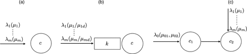
Notes. (a) . (b) . (c) Markovian tandem queue.
loss queue. Class i patients arrive at rate λi and are served at rate μi once admitted. If there are already c patients in the system, the arriving patients are diverted to other service units.
system with delay effect. Class i patients arrive at rate λi. If an arriving patient is immediately served, her service rate becomes μi. Otherwise, she must wait in the queue and experience a delay, and her service rate is μid instead. This service rate is depreciated from μi through the function f. In our experiments, we assume (i.e., the single-step growth function of Chan et al. 2016), where di is class i’s delay effect. Intuitively, in ICUs, if a patient experiences any delay before treatment, her condition may deteriorate, and she is more likely to stay in the ICU for a longer time. Waiting patients are prioritized based on their class, where class 1 receives the highest priority and class m receives the lowest.
Markovian tandem queue. This system captures the interactions between an ICU and other hospital units. For example, station 1 in our model could be the OR, where patients are operated on before being transferred to the ICU (station 2). There is a stream of patients arriving directly to station 1 at rates λ0, and the service rates at station 1 and station 2 are μ01 and μ02, respectively. Patients of class i can also arrive directly at station 2 at rate λi and be served at rate μi.
We denote the parameter sets of the , and the Markovian tandem queues by , and , respectively. For each system, we generate a large number of instances, exploring a wide range of parameters (see Online Appendix C.1 for details). In total, we generate 4,833 queueing systems, each corresponding to a unique parameter set Θ and congestion risk parameters ().
4.2.2. Deriving Predictive Rules.
We implement our computational framework (Figure 1) for generating interpretable predictive rules for each of the queueing models.
Generate Observations. We first characterize the state space. For an queue, the state is defined as , where is the number of class i patients at time t. In an queue, we fully describe the state by including information regarding whether patients have experienced delays. Thus, the state is defined as , where is the total number of class i patients being served, is the number of class i patients currently being served who experienced delays, and is the number of class i patients in the queue who are currently experiencing delays. For Markovian tandem queues, the state is defined as , where is the number of class 0 patients at station 1, is the number of class 0 patients at station 2 who are transferred from station 1, and is the number of class i patients at station 2. With a slight abuse of notation, we denote states of all three systems by . For each queueing model, we collect all system states as our observations because the state space is finite.
Generate Labels. For each state , we compute the congestion risk using the transient probability matrix (see the discussion following Proposition 1). This leverages the fact that the system is Markovian. The labeling is done by comparing the congestion risk with the threshold α. The complete data matrix is illustrated in Table 1.
|

Table 1. Formulation of a Data Matrix for a Queueing System Instance
| Initial state | True risk |
|---|---|
Train Interpretable ML Model. We train support vector machine models (SVMs) (Pisner and Schnyer 2020) with linear kernel2 for each instance.3 We set the features to be the state . In contrast to typical applications of ML, we use the entire data set for training and evaluation, leveraging the fact that the enumeration of the state space is computationally feasible for the three queueing systems. Finally, we train two SVM models for each queueing system that differ by whether observations are weighted by the steady-state distribution of the respective states (“weighted SVM”) or not (“unweighted SVM”).
Evaluate Performance. We evaluate the performance of the trained SVM models by computing the error rate, FNR, and FPR, where each is either averaged uniformly or weighted by the steady-state distribution, depending on how the SVM model was trained.
4.2.3. Results.
The performance measures for the 4,833 instances are reported in Figure 3. We summarize our key findings.
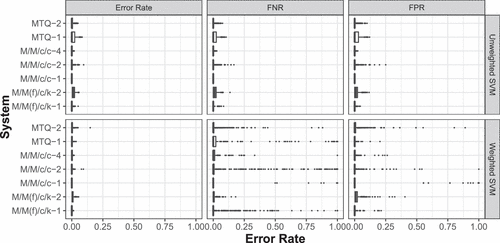
Notes. For each system instance, we compute the error rate, FPR, and FNR under the unweighted and weighted SVM models. The numbers of instances for each queueing model are 304 (), 1,239 (), 166 (), 1,280 (), 627 (), 353 (MTQ – 1), and 864 (MTQ – 2). For all queueing models, the mean error rate is smaller than 3.5%, and the median error rate is very close to 0%.
Interpretability. The generated prediction rules are simple linear functions of the state vector. For example, for the system, the rule is of the form , where are real numbers. These rules can be easily understood by stakeholders. Moreover, the coefficients βi can be used to assess the impact of having an additional patient on the probability of congestion. Note that in general, one could consider alternative interpretable ML models for this task (e.g., Kingsford and Salzberg 2008; Lakkaraju and Rudin 2017; Liu et al. 2022a, b).
Accuracy. In both weighted and unweighted methods, SVM with linear kernel is very accurate in identifying high-risk states with a mean error rate under 4% for all queueing models. The excellent performance suggests an inherent linear structure of the decision boundary separating low- and high-risk states in the studied Markovian queueing systems. Predicting high-risk states only requires tracking the number of patients from each class in each station, regardless of the complex queueing dynamics.
Choice of sample weights in learning methods. The choice of sample weights to penalize misclassified observations depends on the goal. An unweighted learning method might be more suitable when the main concern is the raw count of misclassified observations, whereas a weighted learning method is ideal when the long-run performance is more relevant. Importantly, this choice does not trade off performance, as we observe high accuracy for both approaches. We note that in the training of the weighted models, the penalty parameter (up to 103 in our experiments) is multiplied by the steady-state probability of each observation (i.e., state of the system), which could be very small (in the order of 10−15); this results in prediction errors. Indeed, we observe positive error rates (FPR and FNR) for the model, which was shown to be linearly separable (Proposition 1), under the weighted SVM in the lower row of Figure 3. This problem can be resolved by tightly tuning the ML model (using a higher penalty). Therefore, the reported error rates are conservative.
5. Deriving Rules for Non-Markovian Models
Although Markovian models are frequently used to capture the essence of ICUs’ complex dynamics, their modeling capacity is naturally limited. We are therefore interested in studying more realistic models. We consider an ICU-post intensive care unit (PCU) tandem queueing model of a cardiovascular (CV) surgery practice (Marmor et al. 2013). The queueing model was built using historical data, and it was validated and shown to be accurate through extensive computational experiments. Among the features typically present in general ICUs, this model includes the following: time-varying arrival rates, general LOS distributions, availability of a step-down unit for PCU, and the probability of a patient bouncing back from PCU to ICU. We find that despite the complexity of this queueing model, linear classifiers based on generalized, yet still interpretable, features can accurately predict congestion risk. Specifically, our features represent patients’ count in different stages of the system based on their remaining LOS (i.e., their remaining workload contribution).
We begin this section by introducing the ICU-PCU setting in detail in Section 5.1. In Section 5.2, we describe our approach to predict congestion risk in this non-Markovian setting and report on its performance in Section 5.3. In Section 5.4, we analyze the impact of making surgery rescheduling decisions based on the prediction of risk derived from our approach. Finally, in Section 5.5, we evaluate the impact of model misspecification (i.e., when there is a gap between the real system and the queueing model used as the data-generating process in our approach) on performance.
5.1. The ICU-PCU Tandem Queueing Model
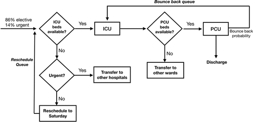
The patient flow in the ICU-PCU is shown in Figure 4. Patients arrive at the medical facility for CV surgery as either elective (scheduled) patients (86% of cases) or as urgent cases (14% of cases). Upon arrival, if an ICU bed is available, the patient proceeds to surgery followed by a transfer to the ICU. Otherwise, if the ICU is full, then incoming urgent patients are transferred to a different hospital, whereas incoming elective patients are rescheduled. Specifically, surgeries initially scheduled for Monday and Tuesday are rescheduled to the upcoming Saturday, whereas surgeries initially scheduled for Wednesday to Friday are rescheduled to the next Saturday. After treatment in the ICU, patients are transferred to the PCU. If the PCU is full, patients are transferred to other hospital wards. A certain percentage of patients may “bounce back” or be readmitted to the ICU from the PCU if their condition deteriorates. Bounce-back patients stay in the PCU until there is an ICU bed available. There are in total six heterogeneous patient classes. The total capacity of the ICU is 28 beds, and the capacity of the PCU is 50 beds. The ICU is most congested on Wednesdays and Thursdays, the days with the most last-minute surgery cancellations. Details of the patients and system performance can be found in Online Appendix C.2, with all model parameters given by Marmor et al. (2013).
5.2. Predicting Risk of Future Congestion
In order to preemptively handle overcrowding and reduce patients’ inconvenience because of rescheduling, we set the goal of predicting the risk of congestion ahead of time. Specifically, at the end of each Saturday, we predict the risk of congestion in the upcoming week. We implement our computational framework as follows.
Generate Observations. We first describe our modeling of the state space. The system state has three components, each capturing information about the ICU, PCU, and the queue of rescheduled patients. Because the system is non-Markovian, we need to record patients’ history, including their time in the current unit (ICU/PCU) or queue (rescheduled queue). The complete state description is available in Online Appendix C.2.
Using the simulation model (Figure 4), we sample a total of 1,000 random Saturdays as follows. First, we generate 10 sample paths starting from an empty system. For each sample path, after a warm-up period, we extract 100 sequential Saturdays along the path. We choose to sample the state of the system on Saturday (i.e., make congestion risk predictions for Saturdays) because in practice, surgery rescheduling policies are based on Saturday’s available capacity. Later, in Section 5.4, we analyze the value of rescheduling surgeries based on Saturday’s predicted congestion risk.
Generate Labels. For each sampled Saturday with state , we simulate 1,000 sample paths starting from that Saturday for seven days. Along the seven-day sample path, we record the ICU occupancy levels at the end of each day. The day-specific congestion risk is estimated by the sample average of the respective indicator:
Table 2 illustrates the data generated using the queueing model, where each row corresponds to a system state on Saturday () and columns correspond to congestion-related metrics for all 1,000 sample paths. For simplicity, the state is numbered sequentially rather than fully specified in the high-dimensional space. The column holds the occupancy levels τ units of time later in each of the sample paths, and the column (with g = 18 in this example) indicates whether the system is congested at the respective time at the corresponding sample path. The last column shows the ground-truth risk, which is a latent variable in practice; it is estimated by averaging across all sample paths.
|
Table 2. An Example of Simulated ICU Data from the Queueing Model
| Initial state Z0 | Future occupancy | Future congestion | True risk |
|---|---|---|---|
| 1 | 20, …, 15 | 1, …, 0 | 0 |
| 2 | 12, …, 27 | 0, …, 1 | 1 |
| ... | ... | ... | 0 |
| 1,000 | 15, …, 17 | 0, …, 0 | 0 |
Notes. Columns and values report the values for all 1,000 sample paths. The last column reports the true risk computed using all 1,000 sample paths for each state .
Generate Interpretable Features. Using the information in the state (patients class, location, time since the start of service, bounce back, etc.), we construct summary features based on patients’ RLOS and stage in the service process. These will be later used to train an interpretable ML model. Specifically, we take the following three steps.
Creating RLOS profiles (Figure 5). We first create a data matrix with information about patients at various stages of service in the system (that is, their unit, class, bounce-back flag, and elapsed service time). We uniformly discretize the elapsed service time to 20 values according to the quantiles of the LOS distribution (e.g., if the processing time of a certain activity is uniformly distributed between 0 and 21 days, the elapsed time can then take the values 1, …, 20 days). In total, we obtain 480 possible patient status vectors (illustrated in the first column of Figure 5). Then, for each patient status vector, we simulate 1,000 potential values of RLOS and represent the cumulative RLOS probability distribution with a 125-dimensional vector (illustrated in the second column of Figure 5). Specifically, the CDF vector contains the probabilities estimated from the simulation, where t ranges from 0.2 to 25 days (with increments of 0.2 days). We then apply hierarchical clustering using the RLOS cumulative distribution vectors as features and generate three RLOS profiles. Figure 5 shows the average CDF value of each RLOS profile. The CDF of the RLOS profile 1 captures those patients who are soon to be discharged, whereas profiles 2 and 3 capture patients who will be in the unit for a moderate time and a longer time, respectively. We note in passing that in cases where patients in the PCU and ICU require dramatically different care, one could do a more granular clustering to capture the recovery time nuances of each subpopulation.
Assigning patients to RLOS profiles. We construct an auxiliary sparse decision tree model that classifies patients to RLOS profiles based on the patient status vector. Specifically, we employ generalized and scalable optimal sparse decision trees (GOSDTs) built by optimizing various objectives rather than using traditional greedy algorithms (see Lin et al. 2020). We applied the GOSDT algorithm in Python using the GOSDT package and varied the regularization parameter to obtain trees of various sizes (for example, Figure C4 in Online Appendix C.2 shows a prediction rule of size 4 represented by either a decision tree or a rule list). The end result of this step is a decision tree that returns the RLOS profile given a patient status vector by applying a series of if-then rules.
Creating summary features. Each state is transformed into a summary feature vector . First, we relabel each patient in the current system to her RLOS profile using the auxiliary model trained in the previous step. Second, we count the number of patients from each RLOS profile at each unit. That is, , where and are the numbers of RLOS profile i patients in ICU and PCU, respectively.
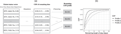
Notes. (a) Clustering to create RLOS profiles. (b) RLOS profiles CDFs.
This feature-engineering approach ensures that the features used by the model to predict congestion risk have an intuitive meaning (i.e., patient count for each RLOS profile) and that their values can be explained using the auxiliary decision tree model obtained in step (2). We note that patients can be assigned to RLOS profiles (clusters) by finding similar status vectors (the first column of Figure 5) and using the mapping formed by the hierarchical clustering. However, this approach is arguably not very interpretable in practice as it relies on the proximity of the RLOS distribution. Step (2) and the creation of the auxiliary model bring interpretability to the assignment of patients to RLOS profiles as it is based on a sparse rule list applied to the patient’s status vector information (instead of on the proximity of the RLOS distribution). We later show that features that summarize patients’ remaining workload are instrumental to accurate prediction and that the use of the auxiliary model only mildly impacts prediction accuracy.
Train Interpretable ML Model. Once the summary features are constructed, we can train ML models to predict risk based on the composition of RLOS profiles. To test the robustness of our approach, we run several prediction tasks for different values of g, α, and τ. For each task, the training data consist of 1,000 sample Saturdays for which we computed the summary features and the estimated risk label . Similarly to Section 4, we trained linear SVM models for each prediction problem and evaluated various accuracy metrics. Specifically, we used the following parameters. We predict the risk of the most congested days, which are Tuesday through Friday (). Assuming that the ICU is considered congested if the occupancy level exceeds 80% of the total capacity, we set the congestion threshold to be . We also choose multiple values of α such that the percentage of high-risk states ranges from 0.2 to 0.8. In total, there are 28 prediction tasks that differ in τ and α.
Evaluate Performance. We use 10-fold cross-validation to perform hyperparameter tuning (of the cost parameter of the trained SVM model) and use a separate test set to estimate prediction accuracy.
We evaluate the following approaches: model-based methods, which are variants of our approach that rely on the queueing model representation of the real system, and data-driven methods, which are included as a proxy for commonly used benchmarks. These methods make predictions directly by constructing ML models using historical data without relying on queueing models. In lieu of historical data as the input data for the data-driven approach, we use a single sample realization of occupancy to represent the actual evolution of the system τ periods ahead starting from each state . That is, there is only a single possible realization for the value of and (i.e., a single path for each state in Table 2). This is in contrast to the model-based approach, which relies on the queueing model to simulate data (i.e., many sample paths) for the possible values of and from each state . We denote the methods by X-Y-Z, where X indicates whether the corresponding method is data driven (data) or model based (Q), Y represents the feature set, and Z is the ML model used. We evaluate the following benchmarks.
Data-counts-logistic. A logistic regression (LR) model trained using features that count the number of patients of each class at each stage for each state . The label for each state corresponds to the realizations of congestion τ periods later (i.e., if the system was congested, and otherwise). The LR model estimates the probability of congestion , and we predict that is high risk if .
Data-counts-quantile. We train a nonparametric quantile regression model (Takeuchi et al. 2006) using the count of patients of each class at each stage as features to estimate the th quantile of . We predict the state as high risk if the th quantile of is greater than or equal to g.
Q-GOSDT-SVM. We employ the model-based approach described earlier in this section. We specifically use the summary features , which are obtained through feature engineering using GOSDT, and train a linear model (SVM) based on these summary features. The hyperparameters of GOSDT were selected using fivefold cross-validation.
Q-counts-SVM. Similar to the previous approach but with the difference of using simple patient counts by class and stage in the system rather than counting the number of patients according to RLOS profiles.
Q-RLOS-SVM. Similar to Q-counts-SVM except that we use RLOS profile counts as features using the assignment of patients to RLOS profiles from the clustering (step (1) in the feature engineering approach). By comparing this benchmark with Q-counts-SVM, we illustrate the value of feature engineering using RLOS profiles. Moreover, comparing this benchmark with Q-GOSDT-SVM shows the potential accuracy loss because of employing an auxiliary model (GOSDT) in step (2) of the feature engineering approach.
5.3. Results
Figure 6 shows the distribution of test error rates across all 28 prediction tasks. Our main findings can be summarized as follows.
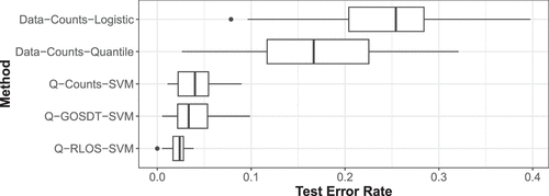
Despite the queueing model’s complexity, the model-based approach is very effective in predicting congestion risk, with both mean and median error rates under 5% for all three model-based approaches. Moreover, it outperforms purely data-driven benchmarks, which report an average error rate approximately six times larger, partly because of having access to the true data-generating process.
Among the three model-based approaches, predictions relying on RLOS profiles (Q-GOSDT-SVM and Q-RLOS-SVM) are generally more accurate than simple user counts (Q-counts-SVM). Although the improvement in this experiment seems modest, in Figures C5 and C6 in Online Appendix C.2, we report on an additional experiment that demonstrates that simply counting patients of different classes is insufficient in general non-Markovian service systems and that incorporating information about remaining workload through the RLOS profiles could significantly improve performance.
There is a trade-off between interpretability and accuracy that can be seen by comparing Q-GOSDT-SVM and Q-RLOS-SVM. The method Q-GOSDT-SVM loses some accuracy by fitting an auxiliary model to make the mapping of the patient status vector to the RLOS profile interpretable. We recall that under Q-RLOS-SVM, on the other hand, the assignment of patients to RLOS profiles relies on the RLOS distribution proximity—which is arguably not very interpretable from a practical standpoint. We note that one can overcome the small loss in accuracy by employing a slightly more flexible auxiliary model in step (2) (e.g., a decision tree with five rather than three leaf nodes).
5.4. Rescheduling Based on Risk Prediction Rules
In this subsection, we demonstrate how a simple policy (Figure 7) based on congestion risk can enhance the system’s performance. Specifically, at the end of each Saturday, we predict the congestion risk of the coming Tuesday, Wednesday, and Thursday. If Tuesday is high risk, we reschedule patients on that day with probability to the following Monday, where ADC stands for advanced cancellation and refers to Tuesday (intuitively, percentage of patients are rescheduled). Notice that advance cancellation is a preventive strategy, in contrast to reactive last-minute cancellations (LMCs in short), which in practice, take a much higher toll on surgeons and patients and incur higher costs. Similarly, we apply risk-based rescheduling to Wednesday () and Thursday ().

Notes. The rows correspond to two consecutive weeks. Tuesday patients are rescheduled with probability to the following Monday, and Wednesday and Thursday patients are rescheduled with probabilities and to the following Saturday.
This preventive policy is parameterized using four values: α, , and . For example, the baseline policy is given by . Figure 8 compares the performance of the baseline policy with five other policies that differ by the value of , which varies between 0% and 40% (the values of and are fixed to 10%, and α is set to 0.8). We observe that in comparison with the baseline policy (where there are 191 LMCs), risk-based rescheduling policies control the trade-off between ADCs and LMCs. Moreover, because the policy intervenes only when congestion is very likely to happen, it can also improve the total number of cancellations (ADC + LMC). We note that although the improvement is relatively modest—in the example, the average LMCs are reduced by 7% from 191 LMCs in the baseline policy to 177 LMCs under = 20%—the preventive policy does not require additional resources, is easy to manage, is minimally disruptive to current practices, and is fully transparent.
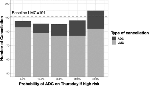
Notes. We evaluate the performance of various preventive policies (varied by on the x axis) by simulating 300 sample paths over 40 consecutive weeks and count the number of LMCs and ADCs for each sample path. The performance of every policy is the mean number of LMCs and ADCs across the 300 sample paths.
5.5. Impact of Model Misspecification
In previous sections, we assume access to a queueing model that precisely represents the real system of interest. However, in practice, the starting point for deriving prediction rules is typically observational data collected directly from the real system instead of an estimated queueing model. Because the estimated queueing model only captures the main dynamics of the real system, a gap between the two is likely to arise. In what follows, we again consider the ICU-PCU setting to compare the model-based and data-driven approaches, this time considering the case where both approaches start from observational data and there is a modeling gap between the real system and the estimated queueing model.
5.5.1. Ground-Truth Queueing Model.
We create a ground-truth queueing model as our real system of interest and use simulation to generate observational data from it. These observational data are the input to the data-driven and model-based approaches. Specifically, the ground-truth queueing model is a modified ICU-PCU system based on Figure 4, in which the flow of patients is affected not only by the occupancy levels inside the ICU and PCU but potentially, also by downstream congestion: that is, by the lack of availability of general inpatient beds within the hospital. We recall that ICU-PCU patients are typically discharged to inpatient units as their condition improves and before they can be discharged. Long and Mathews (2018) show that blocking of ICU patients—when a patient cannot be discharged and moved out from the ICU—because of downstream congestion can result in up to 10% longer LOS. To capture this “slowdown” phenomenon, in the ground-truth model, we consider a 35% probability that a PCU discharge is blocked because of downstream congestion, with a holding period uniformly distributed between 24 and 48 hours. As a result of this blocking period, the LOS of PCU patients is 16% longer than what the patient actually needed. For clarity, we distinguish between the needed PCU LOS (i.e., with no blocking delay) and the actual PCU LOS, which includes the needed LOS plus the blocking delay. Note, however, that the observational data generated from the ground-truth model only indicate patients’ actual PCU LOS, without indicating whether the patient was blocked at the time of discharge. Thus, when employing the model-based approach, we would be utilizing a misspecified queueing model. This is because when estimating the PCU LOS distribution using the observational data from the ground-truth model, we use the actual PCU LOS instead of the needed PCU LOS and completely ignore blocking.
The model misspecification affects the model-based approach in several ways. For example, the incorrect estimation of PCU LOS distribution results in biased RLOS profiles. Recall that in the feature engineering step, we create the RLOS profiles based on simulation. Because the PCU LOS distribution is misspecified, the simulated remaining LOS would be biased, and so are the resulting RLOS profiles (Figure 5).
5.5.2. Comparison of Model-Based and Data-Driven Approaches.
Similarly to Section 5.2, to generate observational data, we first simulate the ground-truth queueing model for a warm-up period and sample the system state at 1,000 random Saturdays. We consider the same set of prediction tasks (28 in total) varied by as in Section 5.2. Given a learning task, for each Saturday, we use the ground-truth model to simulate 1,000 sample paths starting from this Saturday and estimate its true risk label by comparing the sample average congestion probability with the risk threshold α. As before, our objective is to derive a prediction rule that can accurately identify the risk of these 1,000 Saturdays.
Model-Based Approach. We calibrate the ICU-PCU queueing model (Figure 4) with 1,000 days of sample path data simulated from the ground-truth model. For each of the six patient classes, we estimate the arrival rate by weekday and LOS distribution before and after a bounce-back event. As expected, most estimated parameters are quite close to the ground-truth values, but because of model misspecification (ignoring blocking and its effects), the estimated needed PCU LOS is on average 16% longer than the ground-truth needed PCU LOS (i.e., LOS without blocking delay). After we estimate the queueing model parameters, we repeat the model-based learning approach described in Section 5.2 and evaluate the performance of the model-based methods Q-counts-SVM, Q-GOSDT-SVM, and Q-RLOS-SVM. In addition, we evaluate QTrue-RLOS-SVM, which is a model-based approach that assumes access to the ground-truth model (i.e., using the correct queueing model with no misspecification). We use the ground-truth model to simulate risk labels and needed PCU LOS to create the RLOS profiles. Hence, neither the risk labels nor the RLOS profiles are biased. Comparing QTrue-RLOS-SVM with Q-RLOS-SVM allows us to estimate how much accuracy is lost because of model misspecification.
Data-Driven Approach. Using the observational data from the ground-truth model, we train a risk prediction rule via logistic regression (data-counts-logistic) and quantile regression (data-counts-quantile), as described in Section 5.2.
Evaluation. We randomly select 70% of the observations (of the 1,000 Saturdays simulated from the ground-truth model) to train the prediction models (model based and data driven), and the remaining 30% are used as out-of-sample data to evaluate the prediction accuracy by comparing the predicted risk with the true risk labels.
Figure 9 shows the distribution of test errors across all prediction tasks. As expected, because of model misspecification, the model-based approaches perform slightly worse than depicted in Figure 6. The reason for the deteriorating performance of Q-GOSDT-SVM is partly because of the bias in RLOS profile labeling. Nevertheless, the model-based approaches still outperform data-driven benchmarks, especially when the relevant features based on RLOS are included in the prediction rule (e.g., Q-RLOS-SVM has an error rate generally below 5%).
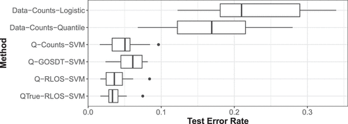
We conclude this section with two practical insights. First, the major advantage of the model-based approach over the data-driven approach is the possibility of generating additional (potentially biased) data, which allows the former to better estimate the latent risk labels. Second, we observe from our experiment that in a large-scale queueing system, even with certain model misspecifications, model-based predictions remain very accurate and outperform data-driven benchmarks significantly.
6. Discussion
We now discuss a few practical considerations for deriving interpretable predictive rules.
Generality of results. Although the theoretical results of Section 4 are limited to fundamental but relatively simple models, the numerical experiments, which consist of a broad set of Markovian models and a large-scale non-Markovian system of ICUs, suggest that our approach works much more generally. It could be used to generate interpretable risk prediction rules for complex queueing models that capture the more intricate dynamics of ICUs.
The advantage in using interpretable rules. Even though our estimation procedure relies on simulation, the end result is an interpretable predictive rule. That is, rather than providing the decision maker a black-box software tool to predict whether a state is low or high risk, the decision maker could be given a laminated card that compactly describes the interpretable predictive rule. The linear rule makes predictions based on the number of patients and their remaining time at the different units, which can be easily understood. Moreover, because we leverage a queueing simulation model, the approach could be applied to very general queueing models that cannot be analyzed theoretically.
The importance of interpretable features. The successful prediction of risk in the large-scale ICU model (Section 5) relies on including interpretable features. Although the specific features may vary across different prediction applications, we believe that our approach of devising aggregate features that capture the system’s remaining workload is essential for achieving good performance under a linear predictive model. Moreover, these features also help to preserve interpretability.
Alternative interpretable ML models. Our theoretical and numerical analyses suggest that linear models can accurately predict congestion risk in ICUs. Such models are simple, interpretable, and widely used in practice. Other methods, such as FasterRisk (Liu et al. 2022b), could improve interpretability further by fitting a linear model with a smaller number of integer coefficients. However, it may be the case that the linear structure is a characteristic of the particular queueing models studied in this work (i.e., models for ICUs) and that, in general, nonlinear models could work better for other queueing systems. In such cases, one may resort to an array of nonlinear interpretable ML models to capture these relations, such as generalized additive models (Liu et al. 2022a), optimal sparse decision trees (Lin et al. 2020), or falling rule lists (Wang and Rudin 2015; see also the surveys by Adadi and Berrada 2018, Rudin et al. 2022, and the references therein).
Scalability. The main computational burden in generating rules stems from estimating risk using Monte Carlo simulation (the time for training and evaluating models is relatively insignificant). Although sufficiently fast for studying the particular models in this paper, in general, one could use more efficient simulation methods (e.g., importance sampling) (see Rubinstein and Kroese 2016), which possibly require fewer simulations from each state. Moreover, more advanced learning techniques (e.g., active learning) (Settles 2009) could help reduce the number of initial states to be simulated. Such improvements could reduce the total running time and lead to more accurate rules. Regardless, simulation of complex systems is routinely done in practice and for research purposes (e.g., Marmor et al. 2013).
Impact of queueing model misspecification on risk prediction. Although our approach relies on an accurate queueing model representation of the real system, its performance is shown to be robust under moderate model misspecification. Moreover, the queueing model-based approach is generally more accurate than data-driven benchmarks in predicting congestion risk. These insights are practically important as fully characterizing a healthcare system is extremely challenging because of its intricate operations, the idiosyncrasy of patient flows, and unobserved decisions (Chan et al. 2016, Long and Mathews 2018). Our approach suggests that even when there is a gap between the estimated queueing model and the real system of interest, our congestion risk predictions can remain fairly accurate.
Alternative risk measures. Although our focus is on predicting the risk of congestion in ICU queueing systems, the estimation procedure is general and could potentially be applied to devise rules for alternative measures across various domains. This can be done by replacing the labels of congestion risk with other measures of choice. For example, one could also formulate the problem of predicting congestion risk over an interval (that is, to predict the likelihood that an undesired event happens in a future interval rather than a single point in time). This could potentially be proxied by creating risk classification models for multiple values of τ.
7. Concluding Remarks
This work studies the problem of predicting congestion risk in ICUs in order to preempt congestion from happening or mitigate its effects. Using a computational framework that is based on queueing theory, simulation, and machine learning, we devise accurate and interpretable predictive rules. Instead of predicting congestion directly from data, our approach takes advantage of the structure of the queueing model representation of the real system to identify high-risk states. Through theoretical and numerical analyses of our approach on a host of established ICU queueing models, we show that the resulting rules are indeed effective and competitive in comparison with various benchmarks. The interpretability of our rules is achieved through the use of interpretable ML models, which in this particular work, take the form of simple conditions that define clusters of patients, and linear models that transform this cluster information into risk predictions. The interpretable clusters capture information about the remaining workload in each system state (e.g., the number of patients in each location aggregated by their remaining LOS profile). The end result is a set of straightforward rules that one can use to assess the status of ICUs to preemptively respond to congestion.
Our work has the following limitations. First, we focus on the prediction problem of anticipating ICU congestion instead of the complete capacity management decision-making problem, which is arguably the ultimate goal. However, we do not necessarily want to automate these decisions. Particularly in healthcare, some critical decisions cannot be accurately modeled or fully automated. This is because relevant information is not always readily available (Herasevich et al. 2016), and decisions typically depend on multiple stakeholders’ knowledge and objectives (e.g., clinical staff and family members). Because the complete decision-making problem cannot be resolved automatically, we strive to provide a simple, accurate, and transparent tool to forecast congestion risk. Second, ideally one would use data from ICUs to validate our approach, but unfortunately, issues, such as missing data and privacy concerns as well as limited access to such environments, prevent most works (including ours) from running such experiments. We instead use extensive simulation models to report on the robustness of our approach.
Overall, we believe that our work demonstrates the potential of using interpretable ML algorithms in conjunction with traditional queueing theory to advance the practice and theory of service operations and could lead to further research in this realm.
1 The definition of risk for a specific state is similar to the concept of value VaR used in finance (Billio and Pelizzon 2000). For a given probability α, VaR measures the maximum possible loss of a portfolio over a certain period after excluding all worse outcomes whose combined probability is at most α. Hence, VaR is equivalent to the congestion threshold g. Indeed, similar to the estimation of VaR with the characterization of the portfolio’s future value, a major challenge in the estimation of congestion risk is characterizing the distribution of the system’s future utilization.
2 We constructed ML models in Python using the scikit-learn package (Pedregosa et al. 2011). The regularization parameter C is tuned from 0.01 to 1,000 in increments of 5 in order to find the best value C with the smallest training error. We briefly note that we also experimented with other models (logistic regression, classification tree, and SVM with polynomial kernel), but SVM with linear kernel performed better in terms of accuracy while preserving interpretability. The code is available upon request from the authors.
3 Prior to learning, we conduct a triviality test to remove instances in which the variation of risk across states is smaller than 10%. Instances with a percentage of high-risk states smaller than 20% or larger than 80% are also removed to avoid trivial results because of imbalanced data sets. We end up with 4,833 instances (of 22,320) for model training. Online Appendix C.1 summarizes descriptive statistics of the generated instances.
References
- (1987) Transient behavior of the M/M/l queue: Starting at the origin. Queueing Systems 2(1):41–65.Google Scholar
- (2018) Peeking inside the black-box: A survey on explainable artificial intelligence (XAI). IEEE Access 6:52138–52160.Google Scholar
- (2018) Comparison of emergency department crowding scores: A discrete-event simulation approach. Health Care Management Sci. 21(1):144–155.Google Scholar
- (2007) Willing to wait?: The influence of patient wait time on satisfaction with primary care. BMC Health Services Res. 7(1):31.Google Scholar
- (2016) Accurate emergency department wait time prediction. Manufacturing Service Oper. Management 18(1):141–156.Link, Google Scholar
- (2015) On patient flow in hospitals: A data-based queueing-science perspective. Stochastic Systems 5(1):146–194.Link, Google Scholar
- (2003) Using neural network rule extraction and decision tables for credit-risk evaluation. Management Sci. 49(3):312–329.Link, Google Scholar
- (2012) Doctors under load: An empirical study of state-dependent service times. Working paper, University of Pennsylvania, Philadelphia.Google Scholar
- (2022) Predicting inpatient flow at a major hospital using interpretable analytics. Manufacturing Service Oper. Management 24(6):2809–2824.Link, Google Scholar
- (2000) Value-at-risk: A multivariate switching regime approach. J. Empirical Finance 7(5):531–554.Google Scholar
- (2020) Mining optimal policies: A pattern recognition approach to model analysis. INFORMS J. Optim. 2(3):145–166.Link, Google Scholar
- (2007) Impact of delayed transfer of critically ill patients from the emergency department to the intensive care unit. Critical Care Medicine 35(6):1477–1483.Google Scholar
- (2016) The impact of delays on service times in the intensive care unit. Management Sci. 63(7):2049–2072.Link, Google Scholar
- (2012) Optimizing intensive care unit discharge decisions with patient readmissions. Oper. Res. 60(6):1323–1341.Link, Google Scholar
- (2017) Disease prediction by machine learning over big data from healthcare communities. IEEE Access 5:8869–8879.Google Scholar
- (2022) Interpretable optimal stopping. Management Sci. 68(3):1616–1638.Link, Google Scholar
- (2007) Modeling the emergency cardiac in-patient flow: An application of queuing theory. Health Care Management Sci. 10(2):125–137.Google Scholar
- (2013) Handbook of Healthcare Operations Management (Springer, New York).Google Scholar
- (1989) Measurements and approximations to describe the offered traffic and predict the average workload in a single-server queue. Proc. IEEE 77(1):171–194.Google Scholar
- (2021) Interpretable machine learning for resource allocation with application to ventilator triage. Preprint, submitted October 21, https://doi.org/10.48550/arXiv.2110.10994.Google Scholar
- (2006) Using queueing theory to increase the effectiveness of emergency department provider staffing. Academic Emergency Medicine 13(1):61–68.Google Scholar
- (2006) A queueing model of activities in an intensive care unit. IMA J. Management Math. 17(3):277–288.Google Scholar
- (1995) Transient characteristics of an system. Adv. Appl. Probab. 27(3):862–888.Google Scholar
- (2016) The future of ICU prediction scores in the era of ‘big data.’ ICU Management Practice 16:70–79.Google Scholar
- (2018) Sharing delay information in service systems: A literature survey. Queueing Systems 89(1–2):49–79.Google Scholar
- (2011) Wait-time predictors for customer service systems with time-varying demand and capacity. Oper. Res. 59(5):1106–1118.Link, Google Scholar
- (2012) An econometric analysis of patient flows in the cardiac intensive care unit. Manufacturing Service Oper. Management 14(1):50–65.Link, Google Scholar
- (1999) Analysis of capacity management of the intensive care unit in a hospital. Eur. J. Oper. Res. 115(1):36–46.Google Scholar
- (2014) ICU admission control: An empirical study of capacity allocation and its implication for patient outcomes. Management Sci. 61(1):19–38.Link, Google Scholar
- (2016) Association among ICU congestion, ICU admission decision, and patient outcomes. Critical Care Medicine 44(10):1814–1821.Google Scholar
- (2008) What are decision trees? Nature Biotechnology 26(9):1011–1013.Google Scholar
- (2001) Asymptotic expansions for the congestion period for the queue. Queueing Systems 39(2):213–256.Google Scholar
- (2015) Stress on the ward: Evidence of safety tipping points in hospitals. Management Sci. 61(4):754–771.Link, Google Scholar
- (2017) Learning cost-effective and interpretable treatment regimes. Proc. 20th Internat. Conf. Artificial Intelligence Statist. (PMLR), 166–175.Google Scholar
- (2022) The risk of algorithm transparency: How algorithm complexity drives the effects on the use of advice. Production Oper. Management 31(9):3419–3434.Google Scholar
- (2015) Interpretable classifiers using rules and Bayesian analysis: Building a better stroke prediction model. Ann. Appl. Statist. 9(3):1350–1371.Google Scholar
- (2020) Generalized and scalable optimal sparse decision trees. Internat. Conf. Machine Learn. (PMLR), 6150–6160.Google Scholar
- (2000) Value at risk. Financial Anal. J. 56(2):47–67.Google Scholar
- (2022a) Fast sparse classification for generalized linear and additive models. Proc. Machine Learn. Res. 151:9304–9333.Google Scholar
- (2022b) Exploring the whole Rashomon set of sparse decision trees. Neural Inform. Processing Systems (NeurIPS).Google Scholar
- (2018) The boarding patient: Effects of ICU and hospital occupancy surges on patient flow. Production Oper. Management 27(12):2122–2143.Google Scholar
- (2019) Questions for artificial intelligence in healthcare. JAMA 321(1):31–32.Google Scholar
- (2013) Recovery bed planning in cardiovascular surgery: A simulation case study. Health Care Management Sci. 16(4):314–327.Google Scholar
MDCalc (2022) Medical calculators, equations, scores, and guidelines. Accessed October 24, 2022, https://www.mdcalc.com/.Google Scholar- (2003) Nineteen dubious ways to compute the exponential of a matrix, twenty-five years later. SIAM Rev. 45(1):3–49.Google Scholar
- (2019) Dissecting racial bias in an algorithm used to manage the health of populations. Science 366(6464):447–453.Google Scholar
- (2011) Scikit-learn: Machine learning in Python. J. Machine Learn. Res. 12:2825–2830.Google Scholar
- (2020)
Support vector machine . Mechelli A, Vieira S, eds. Machine Learning: Methods and Applications to Brain Disorders (Academic Press, London), 101–121.Google Scholar - (2016) “Why should I trust you?” Explaining the predictions of any classifier. Proc. 22nd ACM SIGKDD Internat. Conf. Knowledge Discovery Data Mining (ACM, New York), 1135–1144.Google Scholar
- (1998) Capacity planning for intensive care units. Eur. J. Oper. Res. 105(2):346–355.Google Scholar
- (2012) Refusal of intensive care unit admission due to a full unit: Impact on mortality. Amer. J. Respiratory Critical Care Medicine 185(10):1081–1087.Google Scholar
- (2016) Simulation and the Monte Carlo Method, vol. 10 (John Wiley & Sons, New York).Google Scholar
- (2019) Stop explaining black box machine learning models for high stakes decisions and use interpretable models instead. Nature Machine Intelligence 1(5):206–215.Google Scholar
- (2023) Globally-consistent rule-based summary-explanations for machine learning models: Application to credit-risk evaluation. J. Machine Learning Res. 24(16):1–44.Google Scholar
- (2022) Interpretable machine learning: Fundamental principles and 10 grand challenges. Statist. Surveys 16:1–85.Google Scholar
- (2015) Queue mining for delay prediction in multi-class service processes. Inform. Systems 53:278–295.Google Scholar
- (2009) Active learning literature survey. Technical report, University of Wisconsin–Madison Department of Computer Sciences, Madison, WI.Google Scholar
- (2003) Optimizing admissions to an intensive care unit. Health Care Management Sci. 6(3):131–136.Google Scholar
- (2006) Nonparametric quantile estimation. J. Machine Learn. Res. 7:1231–1264.Google Scholar
- (2003) A First Course in Stochastic Models (John Wiley & Sons, New York).Google Scholar
- (2009) Erlang loss bounds for OT–ICU systems. Queueing Systems 63(1–4):253.Google Scholar
- (2015) Falling rule lists. Proc. 18th Internat. Conf. Artificial Intelligence Statist. (PMLR), 1013–1022.Google Scholar
- (1999) Predicting queueing delays. Management Sci. 45(6):870–888.Link, Google Scholar
- (2017) A data-driven model of an emergency department. Oper. Res. Health Care 12:1–15.Google Scholar
- (2019) Forecasting arrivals and occupancy levels in an emergency department. Oper. Res. Health Care 21:1–18.Google Scholar
- (2013) ICU occupancy and mechanical ventilator use in the United States. Critical Care Medicine 41(12):2712–2719.Google Scholar
- (2016) Using future information to reduce waiting times in the emergency department via diversion. Manufacturing Service Oper. Management 18(3):314–331.Link, Google Scholar
- (2016) Predicting the performance of queues: A data analytic approach. Comput. Oper. Res. 76:33–42.Google Scholar
- (2017) Interpretable classification models for recidivism prediction. J. Roy. Statist. Soc. Series A 180(3):689–722.Google Scholar