Exploiting Data Locality to Improve Performance of Heterogeneous Server Clusters

1. Introduction

Over the last two decades, large-scale load balancing has emerged as a fundamental research problem. In simple terms, the goal is to investigate how to efficiently allocate tasks in large-scale service systems, such as data centers and cloud networks. As modern data centers continue to process massive amounts of data with increasingly stringent processing time requirements, the need for more efficient and scalable, dynamic load-balancing algorithms is greater than ever. The study of scalable load-balancing algorithms started with the seminal works of Adler et al. (1995), Mitzenmacher (1996a, b), and Vvedenskaya et al. (1996), in which the popular “power-of-d choices” or the join-shortest-queue (d) (JSQ(d)) algorithm was introduced. Here, a canonical model was considered that consists of N identical parallel servers, each serving a dedicated queue of tasks. Arriving tasks are routed to the shortest of $d\ge 2$ randomly selected queues by a centralized dispatcher, irrevocably and instantaneously, at the time of arrival. Since then, this model has received significant attention from the research community, and we have seen tremendous progress in our understanding of the performance of various algorithms; see van der Boor et al. (2022) for a recent survey.

Despite this phenomenal progress, when it comes to modern large-scale systems, much of the existing wisdom can be observed to be false. This is primarily because of the fact that the classical model fails to capture two of the most significant factors that impact the performance of these systems. The first is data locality constraints. In simple terms, it means that tasks of a particular type can only be routed to a small subset of servers that are equipped with the appropriate resources to execute them (Tsitsiklis and Xu 2017, Tirmazi et al. 2020, Weng et al. 2020, Rutten and Mukherjee 2022). For example, an image classification request must be routed to a server that is trained with appropriate machine learning models, such as deep convolutional neural network. Also, in online video services like Netflix and YouTube, users’ requests may only be routed to servers that are equipped with the required data (e.g., movies, music). The classical model ignores this effect and assumes full flexibility: that is, that any task can be assigned to any server in the system. In the presence of data locality constraints, the delay performance of the system may degrade drastically as compared with fully flexible systems. The second is heterogeneity in service rates. Servers in any modern large-scale server clusters do not process tasks at equal speeds. This heterogeneity of the service rates is a major bottleneck in implementing the existing heuristics of the classical model. For example, if there are two groups of servers in the system, one faster and the other slower, then popular dynamic algorithms like JSQ(d), which has a provably excellent delay performance when all server speeds are identical, can be observed to be unstable (i.e., their queue lengths blow up) (Mukhopadhyay and Mazumdar 2016, Mukhopadhyay et al. 2016, Gardner et al. 2021, Hurtado-Lange and Maguluri 2021). In other words, heterogeneity shrinks the stability region as formally established in Hurtado-Lange and Maguluri (2021). This happens simply because if all the servers are treated equally, then the slower server pool may receive a higher flow of arrivals than what it can process.

1.1. Takeaway

In summary, both data locality and heterogeneity of server speeds may significantly degrade the system performance. The main contribution of the current work is to establish that when these two aspects are considered together, then the performance can in fact be drastically improved. That is, if servers are heterogeneous, then efficiently designing the data locality constraints (by appropriately placing the resource files in the server network) can regain the full stability region, which was shrunk for fully flexible systems. Moreover, we also establish that carefully designed data locality constraints can ensure the celebrated double-exponential decay of tail probability of the steady-state queue-length distribution even for the heterogeneous systems.

1.2. Our Contributions

Motivated by this, in the current paper, we consider a bipartite graph model for large-scale load-balancing systems, which has recently gained popularity in the research community. In this model, a bipartite graph between the servers and task types describes the compatibility between the two, where an edge represents the server’s ability to process the corresponding task type. This encompasses the classical full-flexibility models as those having a complete bipartite compatibility graph. An immediate difficulty of the new model is that when the graph is nontrivial (i.e., not a collection of isolated pairs or a complete bipartite graph), the mean-field techniques break down. This is because, the queues no longer remain exchangeable, making the aggregate processes, such as the vector of number of servers with queue length i with $i=0,1,2,\dots$, non-Markovian. In addition, we also consider that each dispatcher handles the arrival flow of one of K possible task clusters and that there are M server types. The rate of service at a server depends on its type. Throughout the paper, the key quantity of interest will be the global occupancy process ${\mathbf{q}}^N(t)=(q_{m,l}^N(t),m=1,\dots ,M,l\ge 1)$, where $q_{m,l}^N(t)$ represents the fraction of servers of type m with queue length at least l at time t in the Nth system with N servers, and we will look at the large-system asymptotic regime: $N\to \infty$.

Because of the compatibility constraints, the servers become nonexchangeable, even if they belong to the same type. This causes most of the existing frameworks to break down; see, for example, Mitzenmacher (1996b), Ethier and Kurtz (2009), and Stolyar (2015). To characterize the process-level limit of the queue-length process, we resort to the theory of weakly interacting particle systems and asymptotically couple the evolution of the N-dimensional vector of queue lengths with an appropriately defined infinite system of independent McKean–Vlasov processes; see, for example, Sznitman (1991) and Méléard (1996). We also show the asymptotic independence of any finite number of queue-length processes, also known as the propagation of chaos property. This convergence of the queue-length processes (in L₂ sense) is then used to establish the transient convergence of the occupancy process. One downside of the convergence is that it depends on the assumption that the initial queue lengths within each set of servers of the same type are independent and identically distributed (i.i.d.) and are independent across the set of servers of different types. Because of this assumption, this convergence result cannot be used to establish the interchange of $t\to \infty$ and $N\to \infty$ limits, which is crucial in studying the limit of steady states.

To overcome this issue, we use the framework of Rutten and Mukherjee (2022), recently introduced in the context of homogeneous systems. Here, a notion called proportional sparsity for graph sequences was introduced, which ensures that the empirical queue-length distribution within the set of compatible servers of any dispatcher is close to the empirical queue-length distribution of the entire system. This was used in Rutten and Mukherjee (2022) to construct conditions on graphs that match the performance of a fully flexible system. In the current setup, however, this notion is inadequate because our goal is not to match the performance of the fully flexible system (which is usually poor under heterogeneity). That is why we extend this notion to what we call the clustered proportional sparsity for a sequence of graphs with increasing size to accommodate the heterogeneous systems. The clustered proportional sparsity property allows us to construct a stochastic coupling between the system and another intermediate system whose task allocation is done by a carefully constructed algorithm called global weighted shortest queue (GWSQ(d)) (Algorithm 1). This coupling with the intermediate system, along with clustered proportional sparsity, helps us establish that if the initial occupancy of two systems is close, then the distance (in the ${\mathcal{\ell }}_1$-norm) between their global occupancy remains small uniformly over any finite time interval. In turn, it implies that their limits of the global occupancy systems are the same. As a consequence, we can remove the i.i.d. assumption of the initial queue lengths because this guarantees that under clustered proportional sparsity, the convergence of the occupancy process depends only on the initial occupancy and not on how the individual queues are distributed.

The process-level limit result shows that the transient limit of the occupancy process can be described as a system of ODEs that depend on various graph parameters. Next, we also show that the interchange of limits holds and that the sequence of occupancy states in stationarity converges weakly to the unique fixed point of the ordinary differential equation (ODE). One celebrated feature of the classical JSQ(d) policy for homogeneous systems under full flexibility is that the steady-state queue length decays doubly exponentially as ${\lambda }^{(d^i-1)/(d-1)}$, where $\lambda \in (0,1)$ is the load per server (Mitzenmacher 1996b, Vvedenskaya et al. 1996). We establish this double-exponential decay property for the heterogeneous system.

It is worthwhile to note that the strength of the results lies in that they hold for arbitrary deterministic sequences of graphs satisfying certain properties. However, we show that all these properties are satisfied almost surely by a sequence of inhomogeneous random graphs (irgs) with parameters prescribed by the theorems. This makes it easy to design graphs with the desired favorable properties.

1.3. Related Works

The research on task allocation systems with limited flexibility can be traced back to the works of Foss and Chernova (1998) and Turner (1998). Of particular importance to the current work, Foss and Chernova (1998) considered stability properties of the system using the fluid model. Later, Bramson (2011) generalized some parts of the results in Foss and Chernova (1998) to a broad class of JSQ-type systems, including the JSQ(d) policy, via the Lyapunov function approach. Stolyar (2005) considered optimal routing in an output-queued flexible server system, which is essentially the bipartite graph model for the load-balancing system. Here, the author considered a system with a fixed number of servers and dispatchers in the conventional heavy traffic regime and proposed a routing policy that is optimal in terms of server workload. Recently, Cruise et al. (2020) considered load-balancing problems on hypergraphs and proved their stability conditions. The works, however, did not aim to precisely characterize the system performance in the large-scale scenario.

The analysis in the large-scale scenario became prominent in the last decade, with the emergence of its applications to load balancing in data centers and cloud networks. In the full-flexibility setup, the analysis of heterogeneous server systems gained some attention. In this case, Stolyar (2015, 2017) studied the zero-queueing property of the join-idle-queue policy, Mukhopadhyay and Mazumdar (2016) and Mukhopadhyay et al. (2016) analyzed the JSQ(d) policy in heterogeneous systems with processor-sharing service discipline, Hurtado-Lange and Maguluri (2021) studied the throughput and delay optimality properties of JSQ(d), and Bhambay and Mukhopadhyay (2022) studied a speed-aware JSQ policy. The works on the JSQ(d) policy observe that the stability region shrinks if the dispatcher applies the JSQ(d) policy blindly. One way to mitigate this performance degradation is to take the server speeds into consideration while sampling servers or while assigning tasks to the sampled servers. Such a “hybrid JSQ(d)” scheme is able to recover the stability region. The current work can be contrasted with this approach. First, in the presence of data locality, both the server speeds and the underlying compatibility constraints need to be taken into account during the sampling procedure, and the approach becomes significantly more complicated. Second, we show how exploiting the data locality, the blind JSQ(d) policy can recover the stability region and even achieve the double-exponential decay of tail probabilities of the steady-state queue-length distribution. One advantage of the latter approach is that the dispatchers can be oblivious to the server speeds, which reduces the implementation complexity and also, makes it robust against changes to the servers (e.g., when servers are added/removed).

Recently, Allmeier and Gast (2022) studied the application of (refined) mean-field approximations for heterogeneous systems. Their method is using an ODE to approximate the evolution of each server, and the error vanishes as the system scales. However, this method cannot be directly used in our case. Because of the bipartite compatibility graph structure, it is hard to capture the interactions between two servers, which means that we cannot write the transition rates of the underlying Markov chain as Allmeier and Gast (2022) does. Also, one important assumption in their work is the finite buffer, but we consider the infinite buffer case here.

The aspect of task-server compatibility constraints in large-scale load balancing and scheduling gained popularity only recently, as the data locality became prominent in data centers and cloud networks. This led to many works in this area (Tsitsiklis and Xu 2013, 2017; Gast 2015; Mukherjee et al. 2018a; Budhiraja et al. 2019; Weng et al. 2020; Rutten and Mukherjee 2022). All these works consider homogeneous processing speeds at the servers. The initial works of Turner (1998) and Gast (2015) focused on certain fixed-degree graphs and showed that the flexibility to forward tasks to even a few neighbors with possibly shorter queues may significantly improve the waiting time performance as compared with dedicated arrival streams or a collection of independent M/M/1 queues that the system has a Poisson arrival process, an exponential service time distribution, and one server. Tsitsiklis and Xu (2013, 2017) considered asymptotic optimality properties of the bipartite graph topology in an input-queued, dynamic scheduling framework. Later, in the (output-queued) load-balancing setup, Mukherjee et al. (2018a) considered the JSQ policy, and Budhiraja et al. (2019) considered the transient analysis of the JSQ(d) policy on nonbipartite graphs. The goal in these papers was to provide sufficient conditions on the graph sequence to asymptotically match the performance of a complete graph. Here, we should mention that the nonbipartite graph model cannot be used to capture the data locality constraints. In the presence of data locality constraints, the analysis of the JSQ(d) policy for homogeneous systems, including both transient and interchange of limits, was performed by Rutten and Mukherjee (2022). Weng et al. (2020) is the first to consider the large-scale heterogeneous server model under data locality. They showed that the join-the-fastest-shortest-queue and join-the-fastest-idle-queue policies achieve asymptotic optimality for minimizing mean steady-state waiting time when the bipartite graph is sufficiently well connected. However, these results fall in the category of JSQ-type policies, where the asymptotic behavior is degenerate in the sense that the queue lengths at servers can be either zero or one. Naturally, the results and their analysis are very different from the JSQ(d)-type policies where queues of any length are possible.

1.4. Notations

Let ${\mathbb{N}}_0=\mathbb{N}\cup \{0\}$. For a set S, its cardinality is denoted as $|S|$. For a polish space $\mathcal{S}$, the space of right continuous functions with left limits from $[0,\infty )$ to $\mathcal{S}$ is denoted as $\mathbb{D}([0,\infty ),\mathcal{S})$, endowed with the Skorokhod topology. The distribution of $\mathcal{S}$-valued random variable X will be denoted as $\mathcal{L}(X)$. For a function $f:\hspace{0.17em}[0,\infty )\to \mathbb{R}$, let ${\Vert f\Vert }_{*,t}≔{\sup }_{0\le s\le t}|f(s)|$. The distribution of $\mathcal{S}$-valued random variable X will be denoted as $\mathcal{L}(X)$. For $x\in \mathcal{S}$, the Dirac measure at the point x is denoted as δ_x. ${\Vert ·\Vert }_p$ represents the ${\mathcal{\ell }}_p$-norm. Define $\left(\begin{array}{c}X\\ Y\end{array}\right)=\frac{X(X-1)\cdots (X-Y+1)}{Y!}$ if $X\ge Y$ and is zero otherwise. RHS is the acronym of right-hand side.

2. Model Description

The model for large-scale systems with limited flexibility was considered by Tsitsiklis and Xu (2013, 2017) in the context of scheduling algorithms for input-queued systems. Subsequently, it was considered in Mukherjee et al. (2018a), Budhiraja et al. (2019), Weng et al. (2020), and Rutten and Mukherjee (2022) for output-queued load-balancing systems. Let $G^N=(W^N,V^N,E^N)$ be a system with N single servers, each serving its own queue, and W(N) dispatchers, each handling the assignment of tasks of one type, where $W^N=\{1,\dots ,W(N)\}$ and $V^N=\{1,\dots ,N\}$ denote the sets of dispatchers and servers, respectively. We will interchangeably use the terms task type and dispatcher type throughout the article. Similar to Tsitsiklis and Xu (2013, 2017), we assume that ${\lim }_{N\to \infty } W(N)/N=\zeta$, where $\zeta >0$ is a constant. The set $E^N\subseteq W^N\times V^N$ of edges represents hard compatibility between the dispatchers and servers in the Nth system. In other words, tasks of type i can be assigned to a server j if and only if $(i,j)\in E^N$. Tasks arriving at a dispatcher must be assigned instantaneously and irrevocably to one of the compatible servers.

• Dispatcher clusters. Each dispatcher belongs to one of K possible clusters labeled in $\mathcal{K}=\{1,\dots ,K\}$. Let $W_k^N$ denote the set of all dispatchers in the kth cluster. As $N\to \infty$, assume that $|W_k^N|/W(N)\to w_k\in (0,1)$ for $k\in \mathcal{K}$ with ${\sum }_{k=1}^K{w}_k=1$. Tasks arrive at each dispatcher as an independent Poisson process with rate λ. Note that dispatchers in the same cluster may not have the same set of compatible servers.

• Server types. Based on its processing capability, each server belongs to one of M possible types labeled in $\mathcal{M}=\{1,\dots ,M\}$. The processing time at a type-m server is exponentially distributed with mean $1/u_m$, where u_m is a positive constant. Let $V_m^N$ denote the set of type-m servers, and as $N\to \infty ,|V_m^N|/N\to v_m\in (0,1)$ for $m\in \mathcal{M}$ with ${\sum }_{m=1}^M{v}_m=1$. Throughout, we will assume that asymptotically, the system has sufficient service capacity in the sense that

  $$\lambda \zeta <{\displaystyle \sum _{m\in \mathcal{M}}{u}_m}{v}_m.$$(2.1)

  Note that the left- and right-hand sides represent the scaled total arrival rate and the scaled maximum departure rate, respectively.

For all the asymptotic results, we consider a general class of systems where the compatibility graph satisfies certain asymptotic criteria as specified in Condition 1. Define

Namely, ${\mathrm{deg}}_w^N(i,m)$ is the number of the dispatcher i’s neighboring servers whose type is $m\in \mathcal{M}$. Similarly, ${\mathrm{deg}}_v^N(k,j)$ is the number of the server j’s neighboring dispatchers whose cluster is $k\in \mathcal{K}$.

Condition 1.

The sequence ${\{G^N\}}_{N\ge 1}$ satisfies the following.

1. For each $k\in \mathcal{K}$ and $m\in \mathcal{M}$, let $E^N(k,m)=\{(i,j)\in W_k^N\times V_m^N:(i,j)\in E^N\}$,

   $$\underset{N\to \infty }{\lim }\frac{|E^N(k,m)|}{|W_k^N|\times |V_m^N|}=p_{k,m}\in [0,1].$$(2.2)

   We call the matrix $\mathbf{p}=(p_{k,m},k\in \mathcal{K},m\in \mathcal{M})$ the compatibility matrix.

2. For each $k\in \mathcal{K}$ and $m\in \mathcal{M}$,

   $$\underset{N\to \infty }{\lim }\frac{{\max }_{i\in W_k^N} {\mathrm{deg}}_w^N(i,m)}{{\min }_{i\in W_k^N} {\mathrm{deg}}_w^N(i,m)}=1,\hspace{1em}\underset{N\to \infty }{\lim }\frac{{\max }_{j\in V_m^N} {\mathrm{deg}}_v^N(k,j)}{{\min }_{j\in V_m^N} {\mathrm{deg}}_v^N(k,j)}=1.$$

Intuitively, the condition implies that the “asymptotic density” of edges between cluster-k dispatchers and type-m servers is given by $p_{k,m}$ and that, for each task-cluster-server-type pair, the servers have similar levels of flexibility. The classical, well-studied setup, where any task can be processed by any server, corresponds to the complete bipartite graph with $p_{k,m}^N=1,\hspace{0.17em}\forall k\in \mathcal{K},m\in \mathcal{M}$. In Section 3.5, we show that for any given $\mathbf{p}≔(p_{k,m},k\in \mathcal{K},m\in \mathcal{M})$, a sequence of graphs satisfying Condition 1 can be obtained simply by putting edges suitably randomly. This is a certain class of inhomogeneous random graphs, which we call irg(p); see Definition 3 for details. In fact, the irg(p) sequence of graphs will be proved to satisfy the required conditions for all the results of this article to hold.

2.1. State Space

In the Nth system, let $X_j^N(t)$ be the number of tasks (including those in service) in the queue of server $j\in V^N$ at time t. Let $q_{m,l}^N(t)$ be the proportion of servers of type m with queue length at least l at time t, namely

Let ${\mathbf{q}}^N(t)=(q_{m,l}^N(t),m\in \mathcal{M},l\in {\mathbb{N}}_0)$. Then, ${\mathbf{q}}^N≔{\{{\mathbf{q}}^N(t)\}}_{0\le t<\infty }$ is a process with sample paths in $\mathbb{D}([0,\infty ),\mathcal{S})$, where

is equipped with the ${\mathcal{\ell }}_1$-topology. Note that the space $\mathcal{S}$ is a complete metric space.

2.2. Local JSQ(d) Policy

For any fixed $d\ge 2$, each dispatcher uses the JSQ(d) policy (Mitzenmacher 1996b, Vvedenskaya et al. 1996) to assign the incoming tasks to servers. To describe the policy, define the neighborhood of dispatcher $i\in W^N$, ${\mathcal{N}}_w^N(i)≔\{j\in V^N:(i,j)\in E^N\}$ with ${\delta }_i^N=|{\mathcal{N}}_w^N(i)|$. When a new task arrives at the dispatcher $i\in W^N$ with ${\delta }_i^N\ge d$, it is immediately assigned to the server with the shortest queue among d servers selected uniformly at random from ${\mathcal{N}}_w^N(i)$. Ties are broken uniformly at random. If ${\delta }_i^N<d$, then the task is assigned to one server selected from ${\mathcal{N}}_w^N(i)$ uniformly at random. This ${\delta }_i^N<d$ scenario is asymptotically not relevant for us because all the graphs that we will consider have diverging degrees as $N\to \infty$.

3. Main Results

3.1. Mitigating the Stability Issue

As discussed earlier, when the server speeds are heterogeneous, the fully flexible systems (with the complete bipartite compatibility graph) may not be stable under the JSQ(d) policy, even if we assume that the sufficient service capacity in (2.1) is satisfied. The next lemma provides a necessary and sufficient condition for ergodicity of the queue-length process. Recall ${\delta }_i^N=|{\mathcal{N}}_w^N(i)|$. For any fixed N, define

Lemma 1.

The queue-length process ${(X_j^N(t))}_{j\in V^N}$ under the local JSQ(d) policy is ergodic if and only if ${\rho }^N<1$.

The lemma is an immediate consequence of Foss and Chernova (1998, theorem 2.5); see also Bramson (2011). We omit its proof. Intuitively, ${\rho }^N<1$ means that in the Nth system, for any subset U of servers with possibly long queues (compared with the rest servers), the total rate at which tasks are assigned to some server in this set must be less than the rate of departure from this set.

Because we are interested in large-N behavior, we will assume a certain asymptotic version of the stability criterion. This is fairly standard in the large-system analysis, as one would want to avoid the “heavy traffic” regime when ${\rho }^N\uparrow 1$ as $N\to \infty$. The behavior in the latter scenario is typically qualitatively different from the so-called “subcritical” regime as defined.

Definition 1

(Subcritical Regime). The sequence ${\{G^N\}}_N$ of systems defined is said to be in the subcritical regime with asymptotic load $\rho <1$ if ${\rho }^N\to \rho <1$, as $N\to \infty$.

Throughout this paper, we will assume that the sequence of systems under consideration is in the subcritical regime. From Lemma 1, it is immediate that if a sequence of systems is in subcritical regime, then its queue-length process is ergodic for all large-enough N. The potential nonergodicity of fully flexible, heterogeneous server clusters brings us to the question of when the sufficient service capacity in (2.1) is satisfied, whether we can design the underlying compatibility structure carefully so that the queue-length process is ergodic. In other words, can we regain the stability region? Proposition 1 shows that this is indeed the case. In some sense, this highlights the first-order improvements (i.e., in terms of stability properties) of a careful compatibility structure design in contrast to a fully flexible system.

The establishment of Proposition 1 relies on first building a simple criteria involving the system parameters, which for the sequence of systems satisfying Condition 1, ensures stability for all large-enough N (Lemma 2). Then, we show that given other parameters, a value of ${(p_{k,m})}_{k\in \mathcal{K},m\in \mathcal{M}}$ satisfying this criteria can be found by checking the feasibility region defined by M inequalities. Denote ${\delta }_k≔{\sum }_{m\in \mathcal{M}}{p}_{k,m}{v}_m$ for each $k\in \mathcal{K}$.

Lemma 2.

Let ${\{G^N\}}_N$ be a sequence satisfying Condition 1. The sequence of systems is in subcritical regime if

$$\frac{\lambda \zeta }{u_m}{\displaystyle \sum _{k\in \mathcal{K}}\frac{w_k{p}_{k,m}}{{\delta }_k}}<1,\hspace{1em} \mathit{\text{for}} \mathit{\text{all}} m\in \mathcal{M}.$$(3.1)

Proposition 1.

Let the parameters $\lambda ,\zeta ,d$ and $w_k,v_m,u_m,\hspace{0.17em}k\in \mathcal{K},\hspace{0.17em}m\in \mathcal{M}$, be such that (2.1) is satisfied. Then, there exists ${(p_{k,m})}_{k\in \mathcal{K},m\in \mathcal{M}}\in {[0,1]}^{K\times M}$ such that for any sequence of systems ${\{G^N\}}_{N\ge 1}$ satisfying Condition 1, the queue-length process ${(X_j^N(t))}_{j\in V^N}$ is ergodic for all N large enough. Moreover, such a ${(p_{k,m})}_{k\in \mathcal{K},m\in \mathcal{M}}$ can be obtained explicitly by solving a set of inequalities.

The proof of Proposition 1 is provided in Appendix A.

In the following sections, we will demonstrate, in addition to the first-order improvements, how asymptotic queue-length distribution can be improved as well, for example, in terms of having a double-exponential decay of tail probabilities.

3.2. Process-Level Limit: i.i.d. Case

Our first main result characterizes the process-level limit of the queue-length process $(X_j^N,\hspace{0.17em}j\in V)$, as $N\to \infty$, when the starting states $\{X_j^N(0):j\in V_m^N\}$ are i.i.d. for all $m\in \mathcal{M}$ and independent across different m-values. When the sequence of graphs ${\{G^N\}}_N$ satisfies a stronger condition, called clustered proportional sparsity (Definition 2), the i.i.d. condition can be removed. This is the content of Section 3.3.

Now, note that for a fixed $N\ge 1,\hspace{0.17em}\{X_j^N:j\in V_N\}$ is a system of N interacting stochastic processes, where interactions enter the dynamics through the local empirical measures of neighboring states (the precise dynamics are given in (4.3) and (4.4)). Exploiting tools from the theory of weakly interacting particles, we show in Theorem 1 that as the system size becomes large, queue-length processes converge weakly to those of an infinite system of independent McKean–Vlasov processes $\{X_j:j\in \mathbb{N}\}$ (see, e.g., Sznitman 1991, Méléard 1996). In fact, using a suitable coupling to be described in more detail in Section 4.1, the convergence holds in L₂. For ease of describing such processes and coupling, although we only assumed that certain fractions of servers are of certain types in the model description, it will be convenient to fix the type of each server $j\in \mathbb{N}$ in this subsection by defining a membership map $\mathbf{M}:\mathbb{N}\to \mathcal{M}$, so that $V_m^N=\{j\in V^N:\mathbf{M}(j)=m\}$ with ${\lim }_{N\to \infty }\frac{|V_m^N|}{N}=v_m$ and $V_m={\lim }_{N\to \infty }{V}_m^N$ for each $m\in \mathcal{M}$. With such fixed server types and $X_j^N(0)\equiv X_j(0)$, let

where $\mathbf{M}(j)=m$ and

Here, $\{D_j:j\in V_m\}$ are i.i.d. Poisson processes with rate u_m for each $m\in \mathcal{M},\hspace{0.17em}\{A_j:j\in \mathbb{N}\}$ are i.i.d. Poisson random measures on $[0,\infty )\times {\mathbb{R}}_{+}$ with intensity λdsdy, and all D_j’s and A_j’s are independent. Loosely speaking, A_j corresponds to the arrival processes, and D_j corresponds to the departure processes at servers. $h_t(j,\cdots )$ is the probability that at time t, the server j will receive the new task given the event that the server j is among the d selected servers and the new task is of cluster k. Neglecting d and ζ, $C_j(t)$ can be understood as the probability that the server j will receive the new task. We note that the existence and uniqueness of solutions to (3.2) and (3.3) can be proved by standard arguments (see, e.g., Sznitman 1991, Méléard 1996) using the boundedness and Lipschitz property of the functions b and $x\mapsto {\mathrm{𝟙}}_{(x>0)}$ on ${\mathbb{N}}_0$.

Theorem 1

(Convergence to the McKean–Vlasov Process and Propagation of Chaos). Consider any fixed ${\mathbf{q}}^{\infty }=(q_{m,l}^{\infty },m\in \mathcal{M},l\in {\mathbb{N}}_0)\in \mathcal{S}$. Assume that all $X_j^N(0)$’s are independent, and for each $m\in \mathcal{M},\hspace{0.17em}\{X_j^N(0):j\in V_m^N\}$ is i.i.d. with $\mathbb{P}(X_j^N(0)\ge l)=q_{m,l}^{\infty },\hspace{0.17em}l\in {\mathbb{N}}_0$. On any finite time interval $[0,T]$, T > 0, for any $m\in \mathcal{M}$ and $j\in V_m$, the queue-length process $X_j^N(·)$ at server j weakly converges to the process $X_j(·)$ in (3.2). In fact, one can suitably couple $X_j^N$ with X_j such that

$$\underset{j\in V^N}{\max } \mathbb{E}{\Vert X_j^N-X_j\Vert }_{*,T}^2\stackrel{N\to \infty }{\to }0,$$(3.5)

and hence, the propagation of chaos property holds; that is, for any $n\in \mathbb{N}$ and distinct $j_h\in V_{M_h},\hspace{0.17em}h=1,\dots ,n$,

$$\mathcal{L}(X_{j_1}^N,\dots ,X_{j_n}^N)\stackrel{N\to \infty }{\to }\mathcal{L}(X_{j_1},\dots ,X_{j_n})={\mu }^{M_1}\otimes \cdots \otimes {\mu }^{M_n}.$$(3.6)

Theorem 1 gives us the limit law of all individual queues. Next, in Theorem 2, we will show how such a server-level convergence can be used to obtain a convergence result for the global occupancy process ${\mathbf{q}}^N(·)$ to a deterministic dynamical system, which was our primary goal. The proofs of Theorem 1 and Theorem 2 are provided in Section 4.

Theorem 2

(Process-Level Convergence for i.i.d. Starting State). Assume that all $X_j^N(0)$’s are independent, and for each $m\in \mathcal{M},\hspace{0.17em}\{X_j^N(0):j\in V_m^N\}$ is i.i.d. with $\mathbb{P}(X_j^N(0)\ge l)=q_{m,l}^{\infty },\hspace{0.17em}l\in {\mathbb{N}}_0$ for some ${\mathbf{q}}^{\infty }=(q_{m,l}^{\infty },m\in \mathcal{M},l\in {\mathbb{N}}_0)\in \mathcal{S}$. Then, on any finite time interval, the occupancy process ${\mathbf{q}}^N(·)$ converges weakly with respect to Skorokhod J₁ topology to the deterministic limit $\mathbf{q}(·)≔(q_{m,l}(·),m\in \mathcal{M},l\in {\mathbb{N}}_0)$ given by the unique solution to the following system of ODEs. For all $m\in \mathcal{M},\hspace{0.17em}{q}_{m,0}(t)=1,\hspace{0.17em}{q}_{m,l}(0)=q_{m,l}^{\infty }$, and

$$\begin{array}{l}\frac{d{q}_{m,l}(t)}{dt}=-u_m(q_{m,l}(t)-q_{m,l+1}(t))\hfill \\ +\lambda \zeta (q_{m,l-1}(t)-q_{m,l}(t)){\displaystyle \sum _{k\in \mathcal{K}}\frac{p_{k,m}{w}_k}{{\delta }_k}}\frac{{({\tilde{q}}_{k,l-1}(t))}^d-{({\tilde{q}}_{k,l}(t))}^d}{{\tilde{q}}_{k,l-1}(t)-{\tilde{q}}_{k,l}(t)},\hspace{1em}\forall l\in \mathbb{N}.\hfill \end{array}$$(3.7)

Here, ${\tilde{q}}_{k,l}(t)={\sum }_{m\in \mathcal{M}}\frac{v_m{p}_{k,m}}{{\delta }_k}{q}_{m,l}(t)$ for all $k\in \mathcal{K}$.

Remark 1.

Using the propagation of chaos property (3.6) and the fact that $\{X_j(t):j\in \mathbb{N}\}$ is independent and $\{X_j(t):j\in V_m\}$ is i.i.d. for each $m\in \mathcal{M}$, it follows that the limit of the global occupancy process at any time instant t, in fact, corresponds to the laws of $X_j(t)$ for each type of servers j in (3.2): that is,

$${\mu }_t^m[l,\infty )=\mathbb{P}(X_j(t)\ge l)=q_{m,l}(t),\hspace{1em}j\in V_m,m\in \mathcal{M},l\in {\mathbb{N}}_0,t\ge 0.$$

3.3. Process-Level Limit: General Case

Theorem 2 requires the strong assumption that for each $m\in \mathcal{M},\hspace{0.17em}{X}_j^N(0),\hspace{0.17em}j\in V_m^N$, are i.i.d. In order to argue the interchange of limits, we need to relax this assumption on initial states. This is because the arguments for the interchange of limits involve initiating the prelimit system at the steady state and then showing that as $N\to \infty$, the system must converge to the unique fixed point of the limiting ODE. This requires us to characterize the (process-level) limiting trajectory of the system starting from the arbitrary occupancy state. We achieve this in this section.

Intuitively, the assumption of i.i.d. in Theorems 1 and 2 ensures that the local occupancy observed by any dispatcher $i\in W_k^N,\hspace{0.17em}k\in \mathcal{K}$ is “close,” in suitable sense, to the average occupancy at the entire system. This phenomenon can be ensured asymptotically, even without the i.i.d. assumption, if the graph sequence satisfies a property we call the clustered proportional sparsity. This notion was first introduced for the homogeneous systems in Rutten and Mukherjee (2022). The definition is a modified notion that is suitable for the current heterogeneous setting.

Definition 2

(Clustered Proportional Sparsity). Recall ${\mathcal{N}}_w^N(i)=\{j\in V^N:(i,j)\in E^N\}$. The sequence ${\{G^N\}}_N$ is called clustered proportionally sparse if for any $\epsilon >0$,

$$\underset{k\in \mathcal{K}}{\sup } \underset{U\subseteq V^N}{\sup }\left|\left\{i\in W_k^N:|\frac{|{\mathcal{N}}_w^N(i)\cap U|}{|{\mathcal{N}}_w^N(i)|}-\frac{|E_k^N(U)|}{|E_k^N(V^N)|}|\ge \epsilon \right\}\right|/|W_k^N|\stackrel{N\to \infty }{\to }0,$$(3.8)

where $E_k^N(U)≔\{(i,j)\in W_k^N\times U:(i,j)\in E^N\}$.

Remark 2.

We can view the subset U in the definition as a test set, say $U={\mathcal{Q}}_{m,l}^N(t)$, where ${\mathcal{Q}}_{m,l}^N(t)$ is the set of type $m\in \mathcal{M}$ servers with queue length at least $l\in {\mathbb{N}}_0$ at time t. Hence, Definition 2 ensures that for all but o(N) dispatchers, the observed empirical queue-length distribution within its neighborhood is close to the global weighted empirical queue-length distribution (Definition 4) of its corresponding type. Then, the global occupancy process evolves similarly to (and converges to the same limit as) the case when the initial states are i.i.d.

Theorem 3

(Process-Level Convergence). Let ${\{G^N\}}_N$ be a clustered proportionally sparse sequence of graphs. Assume that ${\mathbf{q}}^N(0)$ weakly converges to ${\mathbf{q}}^{\infty }\in \mathcal{S}$. Then, on any finite time interval, the occupancy process ${\mathbf{q}}^N(·)$ converges weakly with respect to the Skorokhod J₁ topology to the deterministic limit $\mathbf{q}(·)≔(q_{m,l}(·),m\in \mathcal{M},l\in {\mathbb{N}}_0)$ given by the unique solution to the system of ODEs defined by (3.7) with initial state $\mathbf{q}(0)=(q_{m,l}^{\infty },m\in \mathcal{M},l\in {\mathbb{N}}_0)$.

The proof of Theorem 3 is given in Section 4.4.

3.4. Convergence of Steady States

In the last section, we showed the process-level convergence of global occupancy process ${\mathbf{q}}^N(·)$ to a mean-field limit $\mathbf{q}(·)$. In this section, we will establish the convergence of the sequence of stationary distributions to the unique fixed point of the mean-field limit by establishing the interchange of large-N and large-t limits: ${\lim }_{t\to \infty }{\lim }_{N\to \infty }{\mathbf{q}}^N(t)={\lim }_{N\to \infty }{\lim }_{t\to \infty }{\mathbf{q}}^N(t)$. Throughout this section, we will assume that the sequence of systems is in the subcritical regime (recall Definition 1). The first result states that the limiting system of ODEs has a unique fixed point ${\mathbf{q}}^{*}$ and that it satisfies the global stability property (i.e., for any initial point $\mathbf{q}(0)\in \mathcal{S},\hspace{0.17em}{\lim }_{t\to \infty } \mathbf{q}(t)={\mathbf{q}}^{*}$).

Theorem 4

(Global Stability). Let $\overline{\mathbf{q}}(t,{\mathbf{q}}_0)$ be the solution to the system of ODEs in (3.7) with the initial point $\mathbf{q}(0)={\mathbf{q}}_0\in \mathcal{S}$. Then, there exists a unique fixed point ${\mathbf{q}}^{*}=(q_{m,l}^{*},m\in \mathcal{M},l\in {\mathbb{N}}_0)\in \mathcal{S}$ such that ${\lim }_{t\to \infty } \overline{\mathbf{q}}(t,{\mathbf{q}}_0)={\mathbf{q}}^{*}.$

The proof of Theorem 4 is given in Section 5. It relies on a monotonicity property of the system, which ensures that for two processes ${\mathbf{q}}^1(·)$ and ${\mathbf{q}}^2(·)$, if ${\mathbf{q}}^1(0)\le {\mathbf{q}}^2(0)$, then ${\mathbf{q}}^1(t)\le {\mathbf{q}}^2(t)$ for all $t\ge 0$ (see Martin and Suhov 1999, Stolyar 2015).

The last ingredient that we need in order to prove the interchange of limits is to establish tightness of the sequence of random variables ${\{{\mathbf{q}}^N(\infty )\}}_{N\ge 1}$ under a suitable metric, where ${\mathbf{q}}^N(\infty )≔{\lim }_{t\to \infty } {\mathbf{q}}^N(t)$. Here, as before, we should note that the process ${({\mathbf{q}}^N(t))}_{t\ge 0}$ is not Markovian. That is why the random variable ${\mathbf{q}}^N(\infty )$ should be interpreted as the functional applied to the steady-state system. The tightness result is stated in the next theorem.

Theorem 5

(Tightness). For any $\epsilon >0$, there exists a compact subset $\overline{K}(\epsilon )\subseteq \mathcal{S}$, when $\mathcal{S}$ is equipped with the ${\mathcal{\ell }}_1$-topology, such that $\mathbb{P}({\mathbf{q}}^N(\infty )\notin \overline{K}(\epsilon ))<\epsilon ,\hspace{1em}\forall N\ge 1.$

Theorem 5 is proved in Section 5. The key idea is to use the Lyapunov function approach to bound the expected sum of tails $q_{m,l}^N(\infty )$. Combining Theorems 3, 4, and 5, we can prove the following interchange of limits result.

Theorem 6

(Convergence of Steady States). Let ${\{G^N\}}_{N\ge 1}$ be a clustered proportionally sparse sequence of graphs satisfying Condition 1. Then, the sequence of random variables ${\{{\mathbf{q}}^N(\infty )\}}_{N\ge 1}$ converges weakly to ${\mathbf{q}}^{*}$, the unique fixed point of the system of ODEs in (3.7).

One major discovery about the JSQ(d) policy for the classical, homogeneous, fully flexible system is that the limit of the stationary distribution (which in our case, is given by ${\mathbf{q}}^{*}$) has a double-exponential decay of tail (Mitzenmacher 1996b, Vvedenskaya et al. 1996) for any $d\ge 2$. This is in sharp contrast with the (single) exponential decay of the corresponding tail for random routing or d = 1. In fact, in this case, for any $d\ge 2,\hspace{0.17em}{\mathbf{q}}^{*}$ can be characterized explicitly as $q_l^{*}={\lambda }^{\frac{d^l-1}{d-1}}$, where $q_l^{*}$ is the (limiting) steady-state fraction of servers with queue length at least $l=1,2,\dots$. In the current case of heterogeneous systems, it is intractable to characterize the fixed point ${\mathbf{q}}^{*}$ explicitly. However, as stated in the next theorem, we can still prove that the doubly exponential decay of the tails $q_{m,l}^{*}$ for each $m\in \mathcal{M}$ holds.

Theorem 7

(Double-Exponential Tail Decay). Let ${\mathbf{q}}^{*}=(q_{m,l}^{*},m\in \mathcal{M},l\in {\mathbb{N}}_0)$ be the unique fixed point of the system of ODEs in (3.7). Then, for all $m\in \mathcal{M}$, the sequence $\{q_{m,l}^{*},l\in {\mathbb{N}}_0\}$ decreases doubly exponentially; that is, there exist positive constant $l_m\in {\mathbb{N}}_0,\hspace{0.17em}{a}_m\in (0,1)$, and $b_m>0$ such that for all $l\ge l_m,\hspace{0.17em}{q}_{m,l}^{*}\le b_m{a}_m^{d^l}.$

3.5. Simple Data Locality Design Using Randomization

Sections 3.1–3.4 characterize the performance of the occupancy process for arbitrary deterministic sequence of systems where the underlying graph sequence satisfies certain properties. In particular, Condition 1 and Definition 2 provide sufficient criteria under which both the process-level convergence (Theorem 3) and the interchange of limits (Theorem 6) hold. In this section, we show that graphs satisfying the required criteria can be obtained easily if the compatibility graph is designed suitably randomly. Given the asymptotic edge-density parameters in Condition 1, we define a certain sequence of inhomogeneous random graphs or irg as follows.

Definition 3

(irg(p)). Given $\mathbf{p}≔(p_{k,m},k\in \mathcal{K},m\in \mathcal{M})$, the Nth system of irg(p) is constructed as follows. For any $k\in \mathcal{K}$ and $m\in \mathcal{M}$, dispatcher i and server j share an edge with probability $p_{k,m}$ for all $i\in W_k^N$ and $j\in V_m^N$, independently of each other.

For any p for which the asymptotic stability criterion holds, we have the following result for the sequence of irg(p).

Theorem 8.

Let $\mathbf{p}=(p_{k,m},k\in \mathcal{K},m\in \mathcal{M})$ be such that the stability criterion in (3.1) holds and ${\{G_N\}}_{N\ge 1}$ be a sequence of irg(p) with increasing N. Then, the conclusions of Theorems 3 and 6 hold for ${\{G_N\}}_{N\ge 1}$.

The proof of Theorem 8 is provided in Appendix I. It relies on verifying that the sequence of irg(p) graphs satisfies Condition 1 and the property of clustered proportional sparsity almost surely. The verification involves using the concentration of measure arguments to establish structural properties of the compatibility graphs.

4. Proof of Transient Limit Results

In this section, we will prove the results of transient limit results (Theorems 1–3 in Sections 4.2, 4.3, and 4.4, respectively). We start by proving a few auxiliary results in Section 4.1.

4.1. Auxiliary Results

First, we will need a characterization of the evolution of the queue-length process at each server. To describe this evolution, let us introduce the following notations:

To represent the graph, define the edge occupancy ${\xi }_{i,j}^N$ to be the binary variable:

Recall the function b, Poisson processes $\{D_j\}$, and Poisson random measures $\{A_j\}$ in and after (3.4). By Condition 1, for all large-enough N, all dispatchers in the Nth system have at least d neighbors. Hence, without loss of generality, in the rest of this section, we will only consider the case ${\delta }_i^N\ge d,\hspace{0.17em}\forall i\in W^N$. In that case, because of the Poisson thinning property, note that we can write $X_j^N(t)$ as follows:

where

The RHS of the first summation in (4.4) represents the probability that a job arriving at the dispatcher $i\in W^N$ will be assigned to the server $j\in V^N$ given the state $(X_j^N,j\in V^N)$. Moreover, by Condition 1, the term $C_j^N$ for all $j\in V^N$ can be upper bounded, uniformly for all t, by a constant for all large-enough N, which is stated in Lemma 4.

When we do some estimation, like bounding the term $C_j^N$, we need to uniformly bound the number of the neighbors of servers or dispatchers. Such uniformity is stated in Lemma 3 and is a direct result of Condition 1. Recall ${\delta }_i^N=|{\mathcal{N}}_w^N(i)|$ and ${\delta }_k={\sum }_{m\in \mathcal{M}}{p}_{k,m}{v}_m$.

Lemma 3.

For each $k\in \mathcal{K}$,

$$\underset{N\to \infty }{\lim } \underset{i\in W_k^N}{\max }\frac{{\mathrm{deg}}_w^N(i,m)}{|V_m^N|}=\underset{N\to \infty }{\lim } \underset{i\in W_k^N}{\min }\frac{{\mathrm{deg}}_w^N(i,m)}{|V_m^N|}=p_{k,m},\hspace{1em}m\in \mathcal{M},$$(4.5)

and

$$\underset{N\to \infty }{\lim } \underset{i\in W_k^N}{\max }\frac{{\delta }_i^N}{N}=\underset{N\to \infty }{\lim } \underset{i\in W_k^N}{\min }\frac{{\delta }_i^N}{N}={\delta }_k.$$(4.6)

Also, for each $m\in \mathcal{M}$,

$$\underset{N\to \infty }{\lim } \underset{j\in V_m^N}{\max }\frac{{\mathrm{deg}}_v^N(k,j)}{|W_k^N|}=\underset{N\to \infty }{\lim } \underset{j\in V_m^N}{\min }\frac{{\mathrm{deg}}_v^N(k,j)}{|W_k^N|}=p_{k,m},\hspace{1em}k\in \mathcal{K}.$$(4.7)

Lemma 4.

For all large-enough N, we have that for any $m\in \mathcal{M},\hspace{0.17em}j\in V_m^N$, and $t\ge 0$,

$$C_j^N(t)\le 2\zeta d{\displaystyle \sum _{k\in \mathcal{K}}\frac{p_{k,m}{w}_k}{{\delta }_k}}.$$(4.8)

Proof.

By the definition of $C_j^N(t)$, for any $t\ge 0$ and large-enough N,

$$C_j^N(t)\le {\displaystyle \sum _{k\in \mathcal{K}}{\displaystyle \sum _{i\in W_k^N}{\xi }_{i,j}^N}}{\displaystyle \sum _{(j_2,\dots ,j_d)\in {\mathtt{\text{set}}}^N(j)}\frac{{\xi }_{i,j_2}^N\times \cdots \times {\xi }_{i,j_d}^N}{\left(\begin{array}{c}{\delta }_i^N\\ d\end{array}\right)(d-1)!}}={\displaystyle \sum _{k\in \mathcal{K}}{\displaystyle \sum _{i\in W_k^N}{\xi }_{i,j}^N}}\frac{\left(\begin{array}{c}{\delta }_i^N-1\\ d-1\end{array}\right)}{\left(\begin{array}{c}{\delta }_i^N\\ d\end{array}\right)}\le 2\zeta d{\displaystyle \sum _{k\in \mathcal{K}}\frac{p_{k,m}{w}_k}{{\delta }_k}},$$

where the first inequality is because of $b(·)\le 1$ and the last inequality comes from Lemma 3. □

By Lemma 3, we know that the neighborhoods of dispatchers of the same type are almost the same. With the scale of the system size, the local graph structure for each dispatcher of the same type will converge to the average one. The following two lemmas give necessary approximation of the graph structures for large-N systems. Their proofs are combinatorial and are based on Condition 1 and Lemma 3. They are provided in Appendix B.

Lemma 5.

Consider a sequence ${\{G^N\}}_N$ satisfying Condition 1. For each $m\in \mathcal{M}$,

$$\underset{j\in V_m^N}{\max } \underset{k\in \mathcal{K}}{\max } \underset{(M_2,\dots ,M_d)\in {\mathcal{M}}^{d-1}}{\max }|{\displaystyle \sum _{i\in W_k^N}{\xi }_{i,j}^N}{\displaystyle \sum _{\begin{array}{c}(j_2,\dots ,j_d)\in {\mathtt{\text{set}}}^N(j)\\ s.t.\hspace{0.17em}\hspace{0.17em}\hspace{0.17em}\hspace{0.17em}{j}_2\in V_{M_2}^N,\dots ,j_d\in V_{M_d}^N\end{array}}\frac{{\xi }_{i,j_2}^N\times \cdots \times {\xi }_{i,j_d}^N}{\left(\begin{array}{c}{\delta }_i^N\\ d\end{array}\right)(d-1)!}}-\zeta d\frac{p_{k,m}{w}_k}{{\delta }_k}{\displaystyle \prod _{h=2}^d\frac{v_{M_h}{p}_{k,M_h}}{{\delta }_k}}|\stackrel{N\to \infty }{\to }0.$$(4.9)

Lemma 5 states that the probability that the server j in the Nth system will be among the d selected servers when a new task arrives converges to the corresponding probability in the limit system. The argument is mainly based on the law of large numbers (L.L.N.).

Lemma 6.

Consider any $m\in \mathcal{M}$ and $j\in V_m$. For large-enough N,

$${\displaystyle \sum _{i\in W^N}{\displaystyle \sum _{\mathtt{\text{set}}{\mathtt{t}}^N(j)}\frac{{\xi }_{i,j}^N\times {\xi }_{i,j_2}^N\times \cdots \times {\xi }_{i,j_d}^N}{\left(\begin{array}{c}{\delta }_i^N\\ d\end{array}\right)(d-1)!}}}\frac{{\xi }_{i,j}^N\times {\xi }_{i,j_2^{\prime }}^N\times \cdots \times {\xi }_{i,j_d^{\prime }}^N}{\left(\begin{array}{c}{\delta }_i^N\\ d\end{array}\right)(d-1)!}\le \frac{C_1}{N^2},$$(4.10)

where C₁ is a positive constant. Similarly,

$${\displaystyle \sum _{\begin{array}{c}{i}_1,i_2\in W^N,\\ i_1\ne i_2\end{array}}{\displaystyle \sum _{\mathtt{\text{set}}{\mathtt{t}}^N(j)}\frac{{\xi }_{i_1,j}^N\times {\xi }_{i_1,j_2}^N\times \cdots \times {\xi }_{i_1,j_d}^N}{\left(\begin{array}{c}{\delta }_{i_1}^N\\ d\end{array}\right)(d-1)!}}}\frac{{\xi }_{i_2,j}^N\times {\xi }_{i_2,j_2^{\prime }}^N\times \cdots \times {\xi }_{i_2,j_d^{\prime }}^N}{\left(\begin{array}{c}{\delta }_{i_2}^N\\ d\end{array}\right)(d-1)!}\le \frac{C_2}{N},$$(4.11)

where C₂ is a positive constant.

Lemma 6 implies that if we select two elements, say $(j_2,\dots ,j_d),(j_2^{\prime },\dots ,j_d^{\prime })$ independently from ${\mathtt{\text{set}}}^N(j)$, then the probability of $(j_2,\dots ,j_d,j_2^{\prime },\dots ,j_d^{\prime })\in \mathtt{\text{set}}{\mathtt{t}}^N(j)$ is small. (4.10) and (4.11) are used in (4.16).

4.2. Convergence to the McKean–Vlasov Process: i.i.d. Case

Proof of Theorem 1.

It suffices to prove (3.5). Fix any $m\in \mathcal{M},\hspace{0.17em}j\in V_m$, and T > 0. We have that for any fixed $t\in [0,T]$ and any N such that $j\in V^N$,

$$\begin{array}{ll}\mathbb{E}{\Vert X_j^N-X_j\Vert }_{*,t}^2\hfill & \le c_0\mathbb{E}{\Vert X_j^N(t)-X_j(t)\Vert }^2\hfill \\ \hfill & \le c_1\mathbb{E}({\displaystyle {\int }_0^t|}{\mathrm{𝟙}}_{(X_j^N(s)>0)}-{\mathrm{𝟙}}_{(X_j(s)>0)}{|}^{2}ds)+c_1\mathbb{E}{({\displaystyle {\int }_0^t|}{\mathrm{𝟙}}_{(X_j^N(s)>0)}-{\mathrm{𝟙}}_{(X_j(s)>0)}|ds)}^2\hfill \\ \hfill & +c_1\mathbb{E}({\displaystyle {\int }_{[0,t]\times {\mathbb{R}}_{+}}|}{\mathrm{𝟙}}_{(0\le y\le C_j^N(s))}-{\mathrm{𝟙}}_{(0\le y\le C_j(s))}{|}^{2}d\mathit{\text{sdy}})\hfill \\ \hspace{0.17em}\hfill & +c_1\mathbb{E}{({\displaystyle {\int }_{[0,t]\times {\mathbb{R}}_{+}}|}{\mathrm{𝟙}}_{(0\le y\le C_j^N(s))}-{\mathrm{𝟙}}_{(0\le y\le C_j(s))}|\mathit{\text{dsdy}})}^2\hfill \\ \hfill & \le c_1\mathbb{E}({\displaystyle {\int }_0^t|}{X}_j^N(s)-X_j(s){|}^{2}ds)+c_1\mathbb{E}{({\displaystyle {\int }_0^t|}{X}_j^N(s)-X_j(s)|ds)}^2\hfill \\ \hfill & +c_1\mathbb{E}({\displaystyle {\int }_0^t|}{C}_j^N(s)-C_j(s){|}^{2}ds)+c_1\mathbb{E}{({\displaystyle {\int }_0^t|}{C}_j^N(s)-C_j(s)|ds)}^2\hfill \\ \hfill & \le c_2{\displaystyle {\int }_0^t\mathbb{E}}|X_j^N(s)-X_j(s){|}^{2}ds+c_2{\displaystyle {\int }_0^t\mathbb{E}}|C_j^N(s)-C_j(s)|ds,\hfill \end{array}$$(4.12)

where c₀, c₁, and c₂ are positive constants. The first two inequalities are by Doob’s inequalities and Cauchy–Schwarz, respectively. The last inequality comes from the uniform boundedness of $C_j^N(t)$ proved in Lemma 4 and $C_j(t)\le d\zeta$ by the definition. By adding and subtracting terms, we have

$$|C_j^N(s)-C_j(s)|\le |C_j^N(s)-C_j^{N,1}(s)|+|C_j^{N,1}(s)-C_j^{N,2}(s)|+|C_j^{N,2}(s)-C_j(s)|,$$(4.13)

where

$$\begin{array}{l}{C}_j^{N,1}={\displaystyle \sum _{k\in \mathcal{K}}{\displaystyle \sum _{i\in W_k^N}\left[{\xi }_{i,j}^N{\displaystyle \sum _{(j_2,\dots ,j_d)\in {\mathtt{\text{set}}}^N(j)}\frac{{\xi }_{i,j_2}^N\times \cdots \times {\xi }_{i,j_d}^N}{\left(\begin{array}{c}{\delta }_i^N\\ d\end{array}\right)(d-1)!}}b(X_j(s),X_{j_2}(s),\dots ,X_{j_d}(s))\right]}},\hfill \\ C_j^{N,2}={\displaystyle \sum _{k\in \mathcal{K}}{\displaystyle \sum _{i\in W_k^N}[}}{\xi }_{i,j}^N{\displaystyle \sum _{(j_2,\dots ,j_d)\in {\mathtt{\text{set}}}^N(j)}\frac{{\xi }_{i,j_2}^N\times \cdots \times {\xi }_{i,j_d}^N}{\left(\begin{array}{c}{\delta }_i^N\\ d\end{array}\right)(d-1)!}}{\displaystyle {\int }_{{\mathbb{N}}^{d-1}}b}(X_j(t),x_{j_2},\dots ,x_{j_d})\hfill \\ {\mu }_t^{\mathbf{M}(j_2)}(d{x}_{j_2})\cdots {\mu }_t^{\mathbf{M}(j_d)}(d{x}_{j_d})].\hfill \end{array}$$

First, consider $|C_j^N(s)-C_j^{N,1}(s)|$. For large-enough N,

$$\begin{array}{l}\mathbb{E}|C_j^N(s)-C_j^{N,1}(s)|\hfill \\ =\mathbb{E}|{\displaystyle \sum _{k\in \mathcal{K}}{\displaystyle \sum _{i\in W_k^N}[}}{\xi }_{i,j}^N{\displaystyle \sum _{(j_2,\dots ,j_d)\in {\mathtt{\text{set}}}^N(j)}\frac{{\xi }_{i,j_2}^N\times \cdots \times {\xi }_{i,j_d}^N}{\left(\begin{array}{c}{\delta }_i^N\\ d\end{array}\right)(d-1)!}}(b(X_j^N(s),X_{j_2}^N(s),\dots ,X_{j_d}^N(s))\hfill \\ -b(X_j(s),X_{j_2}(s),\dots ,X_{j_d}(s)))]|\hfill \\ \le \mathbb{E}{\displaystyle \sum _{k\in \mathcal{K}}{\displaystyle \sum _{i\in W_k^N}[}}{\xi }_{i,j}^N{\displaystyle \sum _{(j_2,\dots ,j_d)\in {\mathtt{\text{set}}}^N(j)}\frac{{\xi }_{i,j_2}^N\times \cdots \times {\xi }_{i,j_d}^N}{\left(\begin{array}{c}{\delta }_i^N\\ d\end{array}\right)(d-1)!}}(|X_j^N(s)-X_j(s)|+\cdots +|X_{j_d}^N(s)-X_{j_d}(s)|)]\hfill \\ \le d\times \underset{j\in V^N}{\max } \mathbb{E}|X_j^N(s)-X_j(s)|\times {\displaystyle \sum _{k\in \mathcal{K}}{\displaystyle \sum _{i\in W_k^N}{\xi }_{i,j}^N}}{\displaystyle \sum _{(j_2,\dots ,j_d)\in {\mathtt{\text{set}}}^N(j)}\frac{{\xi }_{i,j_2}^N\times \cdots \times {\xi }_{i,j_d}^N}{\left(\begin{array}{c}{\delta }_i^N\\ d\end{array}\right)(d-1)!}}\hfill \\ \le c_3\underset{j\in V^N}{\max } \mathbb{E}|X_j^N(s)-X_j(s)|,\hfill \end{array}$$(4.14)

where c₃ is constant. The first inequality is from that $b(·)$ is Lipschitz continuous with Lipschitz constant 1 and that the last inequality is from (4.9).

Second, consider $|C_j^{N,1}(s)-C_j^{N,2}(s)|$. By Jensen’s inequality, we have ${[\mathbb{E}|C_j^{N,1}(s)-C_j^{N,2}(s)|]}^2\le \mathbb{E}|C_j^{N,1}(s)-C_j^{N,2}(s){|}^2$. Hence, it is sufficient to bound $\mathbb{E}|C_j^{N,1}(s)-C_j^{N,2}(s){|}^2$:

$$\begin{array}{l}\mathbb{E}|C_j^{N,1}(s)-C_j^{N,2}(s){|}^2\hfill \\ =\mathbb{E}|{\displaystyle \sum _{k\in \mathcal{K}}{\displaystyle \sum _{i\in W_k^N}[}}{\xi }_{i,j}^N{\displaystyle \sum _{(j_2,\dots ,j_d)\in {\mathtt{\text{set}}}^N(j)}\frac{{\xi }_{i,j_2}^N\times \cdots \times {\xi }_{i,j_d}^N}{\left(\begin{array}{c}{\delta }_i^N\\ d\end{array}\right)(d-1)!}}b(X_j(s),X_{j_2}(s),\dots ,X_{j_d}(s))]\hfill \\ -{\displaystyle \sum _{k\in \mathcal{K}}{\displaystyle \sum _{i\in W_k^N}[}}{\xi }_{i,j}^N{\displaystyle \sum _{(j_2,\dots ,j_d)\in {\mathtt{\text{set}}}^N(j)}\frac{{\xi }_{i,j_2}^N\times \cdots \times {\xi }_{i,j_d}^N}{\left(\begin{array}{c}{\delta }_i^N\\ d\end{array}\right)(d-1)!}}{\displaystyle {\int }_{{\mathbb{N}}_0^{d-1}}b}(X_j(s),x_{j_2},\dots ,x_{j_d}){\mu }_s^{\mathbf{M}(j_2)}(d{x}_{j_2})\cdots {\mu }_s^{\mathbf{M}(j_d)}(d{x}_{j_d})]{|}^2\hfill \end{array}$$(4.15)

$$\begin{array}{l}\le \mathbb{E}\left[{\displaystyle \sum _{i_1,i_2\in W^N}{\displaystyle \sum _{\mathtt{\text{set}}{\mathtt{t}}^N(j)}\frac{{\xi }_{i_1,j}^N\times {\xi }_{i_1,j_2}^N\times \cdots \times {\xi }_{i_1,j_d}^N}{\left(\begin{array}{c}{\delta }_{i_1}^N\\ d\end{array}\right)(d-1)!}}}\frac{{\xi }_{i_2,j}^N\times {\xi }_{i_2,j_2^{\prime }}^N\times \cdots \times {\xi }_{i_2,j_d^{\prime }}^N}{\left(\begin{array}{c}{\delta }_{i_2}^N\\ d\end{array}\right)(d-1)!}\right]\hfill \\ \stackrel{(a)}{\le }\mathbb{E}[{\displaystyle \sum _{i\in W^N}{\displaystyle \sum _{\mathtt{\text{set}}{\mathtt{t}}^N(j)}\frac{{\xi }_{i,j}^N\times {\xi }_{i,j_2}^N\times \cdots \times {\xi }_{i,j_d}^N}{\left(\begin{array}{c}{\delta }_i^N\\ d\end{array}\right)(d-1)!}}}\frac{{\xi }_{i,j}^N\times {\xi }_{i,j_2^{\prime }}^N\times \cdots \times {\xi }_{i,j_d^{\prime }}^N}{\left(\begin{array}{c}{\delta }_i^N\\ d\end{array}\right)(d-1)!}\hfill \end{array}$$

$$\begin{array}{l}+{\displaystyle \sum _{i_1,i_2\in W^N,i_1\ne i_2}{\displaystyle \sum _{\mathtt{\text{set}}{\mathtt{t}}^N(j)}\frac{{\xi }_{i_1,j}^N\times {\xi }_{i_1,j_2}^N\times \cdots \times {\xi }_{i_1,j_d}^N}{\left(\begin{array}{c}{\delta }_{i_1}^N\\ d\end{array}\right)(d-1)!}}}\frac{{\xi }_{i_2,j}^N\times {\xi }_{i_2,j_2^{\prime }}^N\times \cdots \times {\xi }_{i_2,j_d^{\prime }}^N}{\left(\begin{array}{c}{\delta }_{i_2}^N\\ d\end{array}\right)(d-1)!}]\hfill \\ \le c_4{N}^{-2}+c_5{N}^{-1},\hfill \end{array}$$(4.16)

where the first inequality is because of the fact that $X_j(0)$ is i.i.d. for $j\in V_m$ and independent for different m; so, for each $m\in \mathcal{M},\hspace{0.17em}\{X_j(s),j\in V_m\}$ are also i.i.d., and the independence across the server pools holds for any fixed s > 0. Hence, if $(j,j_2,\dots ,j_d,j_2^{\prime },\dots ,j_d^{\prime })$ are distinct, then

$$\begin{array}{ll}\mathbb{E}[\hfill & (b(X_j(t),X_{j_2}(t),\dots ,X_{j_d}(t))-{\displaystyle {\int }_{{\mathbb{N}}^{d-1}}b}(X_j(t),x_{j_2},\dots ,x_{j_d}){\mu }_t^{\mathbf{M}(j_2)}(d{x}_{j_2})\cdots {\mu }_t^{\mathbf{M}(j_d)}(d{x}_{j_d}))\times \hfill \\ \hfill & (b(X_j(t),X_{j_2^{\prime }}(t),\dots ,X_{j_d^{\prime }}(t))-{\displaystyle {\int }_{{\mathbb{N}}^{d-1}}b}(X_j(t),x_{j_2^{\prime }},\dots ,x_{j_d^{\prime }}){\mu }_t^{\mathbf{M}(j_2^{\prime })}(d{x}_{j_2^{\prime }})\cdots {\mu }_t^{\mathbf{M}(j_d^{\prime })}(d{x}_{j_d^{\prime }}))]=0,\hfill \end{array}$$

and $b(·)$ and $\int b(·)\mu (d·)$ are both in $[0,1]$. The last inequality of (4.16) is by (4.10) and (4.11).

Third, consider $|C_j^{N,2}(s)-C_j(s)|$:

$$\begin{array}{l}\mathbb{E}|C_j^{N,2}(s)-C_j(s)|\hfill \\ =\mathbb{E}|{\displaystyle \sum _{k\in \mathcal{K}}{\displaystyle \sum _{i\in W_k^N}[}}{\xi }_{i,j}^N{\displaystyle \sum _{(j_2,\dots ,j_d)\in {\mathtt{\text{set}}}^N(j)}\frac{{\xi }_{i,j_2}^N\times \cdots \times {\xi }_{i,j_d}^N}{\left(\begin{array}{c}{\delta }_i^N\\ d\end{array}\right)(d-1)!}}{\displaystyle {\int }_{{\mathbb{N}}^{d-1}}b}(X_j(t),x_{j_2},\dots ,x_{j_d}){\mu }_t^{\mathbf{M}(j_2)}(d{x}_{j_2})\cdots {\mu }_t^{\mathbf{M}(j_d)}(d{x}_{j_d})]\hfill \\ -d\zeta {\displaystyle \sum _{k\in \mathcal{K}}\frac{p_{k,m}{w}_k}{{\delta }_k}}{\displaystyle \sum _{(M_2,\dots ,M_d)\in {\mathcal{M}}^{d-1}}{\displaystyle \prod _{h=2}^d\frac{v_{M_h}{p}_{k,M_h}}{{\delta }_k}}}{\displaystyle {\int }_{{\mathbb{N}}^{d-1}}b}(X_j(t),x_{j_2},\dots ,x_{j_d}){\mu }_t^{\mathbf{M}(j_2)}(d{x}_{j_2})\cdots {\mu }_t^{\mathbf{M}(j_d)}(d{x}_{j_d})|\hfill \\ \le c_6(N),\hfill \end{array}$$(4.17)

where $c_6(N)$ only depends on N and goes to zero as $N\to \infty$ and where the inequality comes from (4.9) and the fact that $\int b(·)\mu (d·)\in [0,1]$. Now, by (4.12), (4.13), (4.14), (4.16), and (4.17), we have that for large-enough N,

$$\underset{j\in V^N}{\max } \mathbb{E}{\Vert X_j^N-X_j\Vert }_{*,t}^2\le c_{10}{\displaystyle {\int }_0^t\underset{j\in V^N}{\max }} \mathbb{E}{\Vert X_j^N-X_j\Vert }_{*,t}^{2}ds+f(N),$$

where c₁₀ is a constant and f(N) is a function, which goes to zero as $N\to \infty$. Last, by Gronwall’s inequality, we have (3.5), and this completes the proof. □

4.3. Convergence of the Occupancy Process: i.i.d. Case

In this section, we want to show the convergence of the occupancy process ${\mathbf{q}}^N(·)$ to the limit process q represented by the ODE (3.7). The first step is to investigate the existence and uniqueness of the solution of the ODE (3.7). Define

and clearly, $\mathcal{S}\subseteq \overline{\mathcal{S}}$.

Lemma 7.

If $\mathbf{q}(0)={\mathbf{q}}_0\in \overline{\mathcal{S}}$, then the ODE system (3.7) has a unique solution denoted as $\overline{\mathbf{q}}(t,{\mathbf{q}}_0),\hspace{0.17em}t\ge 0$ in $\overline{\mathcal{S}}$.

The proof of Lemma 7 is based on the Picard successive approximation method (Martin and Suhov 1999, theorem 1(i)) and is provided in Appendix C.

Proof of Theorem 2.

Fix any $T\in (0,\infty )$. For each $m\in \mathcal{M}$, consider random measures ${\mu }_m^N=\frac{1}{|V_m^N|}{\sum }_{j\in V_m^N}{\delta }_{X_j^N(·)}$ and ${\overline{\mu }}_m^N=\frac{1}{|V_m^N|}{\sum }_{j\in V_m^N}{\delta }_{X_j(·)}$ on $\mathbb{S}≔\mathbb{D}([0,T],{\mathbb{N}}_0)$, where $X_j(·)$ is defined in (3.2). Denote the joint measures ${\mu }^N=({\mu }_1^N,\dots ,{\mu }_M^N)$ and ${\overline{\mu }}^N=({\overline{\mu }}_1^N,\dots ,{\overline{\mu }}_M^N)$. Denote by $d_{BL}(·,·)$ the bounded Lipschitz metric for probability measures on $\mathbb{S}$:

$$d_{BL}({\mu }_1,{\mu }_2)≔\underset{{\Vert f\Vert }_{BL}\le 1}{\sup }|{\displaystyle {\int }_{\mathbb{S}}f}d{\mu }_1-{\displaystyle {\int }_{\mathbb{S}}f}d{\mu }_2|,\hspace{1em}{\Vert f\Vert }_{BL}≔\max \left\{{\Vert f\Vert }_{\infty },\underset{x\ne y}{\sup }\frac{f(x)-f(y)}{d(x,y)}\right\}.$$

From (3.5), we have

$$\mathbb{E}{d}_{BL}({\mu }_m^N,{\overline{\mu }}_m^N)\le \mathbb{E}\underset{{\Vert f\Vert }_{BL}\le 1}{\sup }\frac{1}{|V_m^N|}{\displaystyle \sum _{j\in V_m^N}|}f(X_j^N)-f(X_j)|\le \frac{1}{|V_m^N|}{\displaystyle \sum _{j\in V^N}\mathbb{E}}{\Vert X_j^N-X_j\Vert }_{*,T}\stackrel{N\to \infty }{\to }0,$$

which implies that $d_{BL}({\mu }_m^N,{\overline{\mu }}_m^N)\stackrel{\hspace{0.17em}\mathbb{P}\hspace{0.17em}}{\to }0$ for each $m\in \mathcal{M}$. Because ${\overline{\mu }}_m^N\stackrel{\hspace{0.17em}\mathbb{P}\hspace{0.17em}}{\to }{\mu }_m$ by the L.L.N., we have ${\mu }^N=({\mu }_1^N,\dots ,{\mu }_M^N)\stackrel{\hspace{0.17em}\mathbb{P}\hspace{0.17em}}{\to }({\mu }_1,\dots ,{\mu }_M)$ by Slutsky’s theorem. Also, it is easy to check that ${\sup }_N \mathbb{E}[{\sup }_{0\le t\le T}{\Vert {\mathbf{q}}^N(t)\Vert }_{{\mathcal{\ell }}_1}^2]<\infty .$ Thus, we have ${\mathbf{q}}^N\stackrel{\hspace{0.17em}\mathbb{P}\hspace{0.17em}}{\to }\mathbf{q}$. Next, we need to show that q satisfies (3.7). Define $f_l(x)={\mathrm{𝟙}}_{\{x\ge l\}},\hspace{0.17em}l\in {\mathbb{N}}_0$. By (3.2), we have that for any $m\in \mathcal{M}$ and $j\in V_m$,

$$\begin{array}{ll}\mathbb{E}{f}_l(X_j(t))\hfill & =\mathbb{E}{f}_l(X_j(0))+{\displaystyle {\int }_0^t{u}_m}\mathbb{E} {\mathrm{𝟙}}_{\{X_j(s)>0\}}(f_l(X_j(s)-1)-f_l(X_j(s)))ds\hfill \\ \hfill & +{\displaystyle {\int }_0^t{\displaystyle {\int }_{{\mathbb{N}}^{d-1}}\lambda }}\zeta d{\displaystyle \sum _{k\in \mathcal{K}}\frac{p_{k,m}{w}_k}{{\delta }_k}}{\displaystyle \sum _{(M_2,\dots ,M_d)\in {\mathcal{M}}^{d-1}}{\displaystyle \prod _{h=2}^d\frac{v_{M_h}{p}_{k,M_h}}{{\delta }_k}}}\hfill \\ \hfill & \hspace{1em}\hspace{1em}\times \mathbb{E}[b(X_j(s),x_{j_2},\dots ,x_{j_d})(f_l(X_j(s)+1)-f_l(X_j(s)))]{\mu }_s^{M_2}(d{x}_{j_2})\cdots {\mu }_s^{M_d}(d{x}_{j_d})ds\hfill \\ \hfill & =\mathbb{E}{f}_l(X_j(0))+{\displaystyle {\int }_0^t{u}_m}\mathbb{E} {\mathrm{𝟙}}_{\{X_j(s)>0\}}(f_{l+1}(X_j(s))-f_l(X_j(s)))ds\hfill \\ \hfill & +{\displaystyle {\int }_0^t{\displaystyle {\int }_{{\mathbb{N}}^{d-1}}\lambda }}\zeta d{\displaystyle \sum _{k\in \mathcal{K}}\frac{p_{k,m}{w}_k}{{\delta }_k}}{\displaystyle \sum _{(M_2,\dots ,M_d)\in {\mathcal{M}}^{d-1}}{\displaystyle \prod _{h=2}^d\frac{v_{M_h}{p}_{k,M_h}}{{\delta }_k}}}\hfill \\ \hfill & \hspace{1em}\hspace{1em}\times \mathbb{E}[b(l-1,x_{j_2},\dots ,x_{j_d})(f_{l-1}(X_j(s))-f_l(X_j(s)))]{\mu }_s^{M_2}(d{x}_{j_2})\cdots {\mu }_s^{M_d}(d{x}_{j_d})ds.\hfill \end{array}$$

For any $m\in \mathcal{M}$, if $j\in V_m$, then $\mathbb{E}{f}_l(X_j(t))=q_{m,l}(t)={\mu }_t^m[l,\infty )$ for $l=1,2,\dots$. Hence,

$$\begin{array}{ll}{q}_{m,l}(t)\hfill & =q_{m,l}(0)-{\displaystyle {\int }_0^t{u}_m}(q_{m,l}(s)-q_{m,l+1}(s))ds+{\displaystyle {\int }_0^t\lambda }\zeta d{\displaystyle \sum _{k\in \mathcal{K}}\frac{p_{k,m}{w}_k}{{\delta }_k}}(q_{m,l-1}(s)-q_{m,l}(s))\hfill \\ \hfill & \times {\displaystyle \sum _{(M_2,\dots ,M_d)\in {\mathcal{M}}^{d-1}}{\displaystyle \prod _{h=2}^d\frac{v_{M_h}{p}_{k,M_h}}{{\delta }_k}}}{\displaystyle {\int }_{{\mathbb{N}}^{d-1}}b}(l-1,x_{j_2},\dots ,x_{j_d}){\mu }_s^{M_2}(d{x}_{j_2})\cdots {\mu }_s^{M_d}(d{x}_{j_d})ds.\hfill \end{array}$$(4.18)

Also,

$$\begin{array}{ll}\hfill & {\displaystyle \sum _{(M_2,\dots ,M_d)\in {\mathcal{M}}^{d-1}}{\displaystyle \prod _{h=2}^d\frac{v_{M_h}{p}_{k,M_h}}{{\delta }_k}}}{\displaystyle {\int }_{{\mathbb{N}}^{d-1}}b}(l-1,x_{j_2},\dots ,x_{j_d}){\mu }_s^{M_2}(d{x}_{j_2})\cdots {\mu }_s^{M_d}(d{x}_{j_d})\hfill \\ \hfill & ={\displaystyle \sum _{\overline{r}\in \overline{\mathcal{R}}}{\displaystyle \sum _{\overline{r}\prime \in \overline{\mathcal{R}}\prime (\overline{r})}\frac{1}{1+|\overline{r}\prime |}}}{\displaystyle \prod _{m\in \mathcal{M}}\left(\begin{array}{c}{r}_m\\ r_m^{\prime }\end{array}\right)}{\left(\frac{v_m{p}_{k,m}}{{\delta }_k}\right)}^{r_m}{(q_{m,l-1}(s)-q_{m,l}(s))}^{r_m^{\prime }}{(q_{m,l}(s))}^{r_m-r_m^{\prime }}\hfill \\ \hfill & ={\displaystyle \sum _{r=0}^{d-1}\frac{1}{1+r}}\left(\begin{array}{c}d-1\\ r\end{array}\right){\left({\displaystyle \sum _{m\in \mathcal{M}}\frac{v_m{p}_{k,m}}{{\delta }_k}}{q}_{m,l-1}(s)-{\displaystyle \sum _{m\in \mathcal{M}}\frac{v_m{p}_{k,m}}{{\delta }_k}}{q}_{m,l}(s)\right)}^r{\left({\displaystyle \sum _{m\in \mathcal{M}}\frac{v_m{p}_{k,m}}{{\delta }_k}}{q}_{m,l}(s)\right)}^{d-1-r}\hfill \\ \hfill & ={\displaystyle \sum _{r=1}^d\frac{1}{r}}\left(\begin{array}{c}d-1\\ r-1\end{array}\right){({\tilde{q}}_{k,l-1}(s)-{\tilde{q}}_{k,l}(s))}^{r-1}{({\tilde{q}}_{k,l}(s))}^{d-r}\hspace{1em}(\text{Let} {\tilde{q}}_{k,l}(s)={\displaystyle \sum _{m\in \mathcal{M}}\frac{v_m{p}_{k,m}}{{\delta }_k}}{q}_{m,l}(s))\hfill \\ \hfill & =\frac{{({\tilde{q}}_{k,l-1}(s))}^d-{({\tilde{q}}_{k,l}(s))}^d}{d({\tilde{q}}_{k,l-1}(s)-{\tilde{q}}_{k,l}(s))},\hfill \end{array}$$(4.19)

where $\overline{\mathcal{R}}=\{\overline{r}=(r_1,\dots ,r_M)\in {\mathbb{N}}_0^M:{\sum }_{m\in \mathcal{M}}{r}_m=d-1\}$ and $\overline{\mathcal{R}}\prime (\overline{r})=\{\overline{r}\prime =(r_1^{\prime },\dots ,r_M^{\prime })\in {\mathbb{N}}_0^M:r_m^{\prime }\le r_m,\forall m\in \mathcal{M}\}$ given $\overline{r}\in \overline{\mathcal{R}}$. Plugging (4.19) into (4.18), we get the desired result. □

4.4. Convergence of the Occupancy Process: General Case

In this section, we will discuss the case in which the sequence ${\{G^N\}}_N$ is clustered proportionally sparse, which helps us remove the i.i.d. assumption in Theorem 3. Intuitively, if ${\{G^N\}}_N$ is clustered proportionally sparse, then for each $k\in \mathcal{K}$ and each dispatcher $i\in W_k^N$, the queue-length distribution of its neighborhood will always be close (in an appropriate sense) to the corresponding global weighted queue-length distribution (GWQD). Clustered proportional sparsity ensures that this statement holds uniformly for all occupancy states. Loosely speaking, this statement enables us to make sure that the evolution of the occupancy process happens in the same way for any initial state as in the case of the i.i.d. initial state. For the case of homogeneous systems, the notion of proportional sparsity was introduced in Rutten and Mukherjee (2022). Here, proportional sparsity was defined in a way that for most dispatcher i, the fraction of its neighbors within any subset U of servers is proportional to the size of the subset U. However, because of the heterogeneous compatibility between dispatchers and servers, such a fraction, in the current setup, depends on the corresponding type of the dispatcher as well $($see the term $\frac{E_k^N(U)}{E_k^N(V^N)}$ in Definition 2$)$. Thus, unlike the homogeneous case where the local queue-length distribution (LQD) is directly compared with the global queue-length distribution of the system, for the heterogeneous case, we need to define K types of global weighted queue-length distribution (see Definition 4), where the weights are determined by the asymptotic properties of the graph structure: $(v_m,m\in \mathcal{M})$ and $(p_{k,m},k\in \mathcal{K},m\in \mathcal{M})$. Then, we compare the local queue-length distribution of dispatcher i with the global weighted queue-length distribution of the corresponding type as defined.

Definition 4.

Consider any fixed $N\in \mathbb{N}$ and $k\in \mathcal{K}$. Given the global occupancy ${\mathbf{q}}^N=(q_{m,l}^N,m\in \mathcal{M},l\in {\mathbb{N}}_0)$ of the Nth system, the GWQD of cluster k is defined as $(x_{k,m,l}^N,m\in \mathcal{M},l\in {\mathbb{N}}_0)$, where $x_{k,m,l}^N=\frac{v_m{p}_{k,m}}{{\delta }_k}(q_{m,l+1}^N-q_{m,l}^N).$

Also, the local queue-length distribution is defined as follows.

Definition 5.

Consider any fixed $N\in \mathbb{N}$ and $k\in \mathcal{K}$. Given the state $(X_j^N,j\in V^N)$ of the Nth system, the LQD of dispatcher $i\in W_k^N$ is defined as $({\widehat{x}}_{i,m,l}^N,m\in \mathcal{M},l\in {\mathbb{N}}_0)$, where ${\widehat{x}}_{i,m,l}^N=\frac{|\{j\in V_m^N:{\xi }_{i,j}^N=1 \text{and} X_j^N=l\}|}{|{\mathcal{N}}_w^N(i)|}.$

Although the dispatcher following the JSQ(d) policy selects a target server based on its LQD, if its LQD is close (in a suitable sense) to its corresponding GWQD, then the selection can be viewed as if the decision was based on the GWQD. The latter case is easier to analyze. Hence, if a dispatcher’s LQD is close to its corresponding GWQD, we call it a good dispatcher

Definition 6

(ε-Good Dispatcher). Consider any fixed $N\in \mathbb{N}$ and an $\epsilon >0$. Given the state $(X_j^N,j\in V^N)$ of the Nth system, a dispatcher $i\in W_k^N,\hspace{0.17em}k\in \mathcal{K}$, is ε-good if

$${\displaystyle \sum _{m\in \mathcal{M}}{\displaystyle \sum _{l\in {\mathbb{N}}_0}|}}{\widehat{x}}_{i,m,l}^N-x_{k,m,l}^N|\le \epsilon .$$(4.20)

Also, a dispatcher is ε-bad if it is not ε-good.

4.4.1. Consequences of Clustered Proportional Sparsity.

The proof of Theorem 3 relies on the idea that if the local occupancy of each dispatcher within a particular type evolves similar to the global occupancy of that type, then the process-level limiting behavior should not depend on any specific initial state. That is, it will enable us to go beyond the i.i.d. assumption. The first step for this approach to work is to show that almost all dispatchers are ε-good for any $\epsilon >0$. Here is where we need the property of clustered proportional sparsity. This is stated in the next proposition.

Proposition 2.

Let ${\{G^N\}}_N$ be a sequence of clustered proportionally sparse graphs. For any $T\ge 0$ and ${\epsilon }_1,{\epsilon }_2>0$,

$$\mathbb{P}(\underset{t\in [0,T]}{\sup } {\mathcal{ℬ}}_N^{{\epsilon }_1}(t)\ge {\epsilon }_2|W^N|)\stackrel{N\to \infty }{\to }0,$$(4.21)

where ${\mathcal{ℬ}}_N^{{\epsilon }_1}(t)$ is the number of ${\epsilon }_1$-bad dispatchers at time t.

The intuition behind Proposition 2 is that the servers of type $m\in \mathcal{M}$ with queue length $l\in {\mathbb{N}}_0$ form a subset $U_{m,l}^N$ of the server set V^N. If this set is large, then by the clustered proportional sparsity, for any fixed $k\in \mathcal{K}$ and almost all $i\in W_k^N$, the fraction of the dispatcher i’s neighbors within $U_{m,l}^N$ is close to $\frac{|E_k^N(U_{m,l}^N)|}{|E_k^N(V^N)|}$, which is close to $x_{k,m,l}^N$ for large-enough N by Condition 1. Also, in order to deal with the sum over $l\in {\mathbb{N}}_0$, we will need to establish uniform bounds of the tail of the occupancy process on any finite time interval. The complete proof is given in Appendix D.

4.4.2. Coupling with an Intermediate System.

The main methodology for the proof of Theorem 3 is a stochastic coupling with a sequence ${\{G^{\prime N}\}}_{N\ge 1}$ of carefully constructed systems where the evolution of each system $G^{\prime N}$ can be coupled with that of the system G^N. For each N, the system $G^{\prime N}$ has the same sets of dispatchers and servers as G^N (i.e., $W{\prime }^N=W^N$ and $V^{\prime N}=V^N$). However, the task assignment in $G^{\prime N}$ happens differently. To describe the task assignment policy, let us introduce the following notations. Let $X_j^{\prime N}(t)$ be the number of tasks (including those in service) in the queue of server $j\in V^{\prime N}$ at time t. Let ${\mathbf{q}}^{\prime N}(t)=(q_{m,l}^{\prime N}(t),m\in \mathcal{M},l\in {\mathbb{N}}_0)$ be the corresponding global occupancy at time t, which is defined in the same way as ${\mathbf{q}}^N$ for the system G^N. Then, the system $G^{\prime N}$ assigns tasks under the GWSQ(d) policy as described in Algorithm 1. The GWSQ(d) policy is essentially a variant of the JSQ(d) policy because for each new task, the dispatcher selects a target set of servers of size d according to the global weighted queue-length distribution.

Algorithm 1

(GWSQ(d))

while A new task arrives at dispatcher $i\in W_k^N,\hspace{0.17em}k\in \mathcal{K}$ do

 Get the current global occupancy ${\mathbf{q}}^N=(q_{m,l}^N,m\in \mathcal{M},l\in {\mathbb{N}}_0)$;

 Calculate the global weighted queue-length distribution ${\mathbf{x}}_k^N=(x_{k,m,l}^N,m\in \mathcal{M},l\in {\mathbb{N}}_0)$ of cluster k,

$$x_{k,m,l}^N=\frac{v_m{p}_{k,m}}{{\delta }_k}(q_{m,l+1}^N-q_{m,l}^N);$$

 Randomly select a set $\mathtt{\text{selec}}{\mathtt{t}}^N$ with size d as the following.

• Let $Y_{k,m,l}^N(t)\in {\mathbb{N}}_0$ be the number of servers of type $m\in \mathcal{M}$ with queue length $l\in {\mathbb{N}}_0$ in the set $\mathtt{\text{selec}}{\mathtt{t}}^N$;

• $(Y_{k,m,l}^N(t),m\in \mathcal{M},l\in N_0)$ satisfies

  $${\displaystyle \sum _{m\in \mathcal{M},l\in {\mathbb{N}}_0}{Y}_{k,m,l}^N}(t)=d;$$

• the probability of selecting $(Y_{k,m,l}^N(t),m\in \mathcal{M},l\in N_0)$ is

  $$\mathbb{P}(Y_{k,m,l}^N(t),m\in \mathcal{M},l\in N_0)={\displaystyle \prod _{m\in \mathcal{M},l\in {\mathbb{N}}_0}}\left(\begin{array}{c}{X}_{k,m,l}^N(t)\\ Y_{k,m,l}^N(t)\end{array}\right)/\left(\begin{array}{c}N\\ d\end{array}\right);$$
    where $X_{k,m,l}^N=N\times x_{k,m,l}^N$.

 Get $l^{*}=\min (l\in {\mathbb{N}}_0:\exists k\in \mathcal{K},m\in \mathcal{M} \text{such} \text{that} Y_{k,m,l}^N>0)$;

 Assign the task to a type $m\in \mathcal{M}$ server with queue length $l^{*}$ with probability

$$\frac{Y_{k,m,l^{*}}^N}{{\sum }_{m\in \mathcal{M}}{Y}_{k,m,l^{*}}^N}.$$

end

Next, we couple the evolution of the system $G^{\prime N}$ with that of the system G^N by the optimal coupling method. The optimal coupling for two stochastic processes is similar to the maximal coupling for two discrete random variables (say, X and Y), maximizing the probability $\mathbb{P}(X=Y)$.

4.4.2.1. Optimal Coupling.

Fix any N. In both systems, within the pool of servers of each type, arrange the servers in the nondecreasing order of their queue lengths (ties are broken arbitrarily). Now, couple the evolution of the system G^N with the system $G^{\prime N}$ in the following way.

• Departure. For any $m\in \mathcal{M}$ and $n=1,\dots ,|V_m^N|$, synchronize the departure epochs of the nth ordered servers of type m in the two systems.

• Arrival. The coupling of arrivals is the tricky part. For this, first synchronize the arrival epochs at each dispatcher i in both systems $G^{\prime N}$ and G^N. At an arrival epoch of dispatcher $i\in W_k^N$, let $({\widehat{x}}_{i,m,l}^N,m\in \mathcal{M},l\in {\mathbb{N}}_0)$ be the local empirical distribution of dispatcher i in the system G^N and $(x_{k,m,l}^{\prime N},m\in \mathcal{M},l\in {\mathbb{N}}_0)$ be the weighted global empirical distribution of cluster-k dispatchers in the system $G^{\prime N}$. Then, in the system G^N, the probability that the task will be assigned to a server of type $m\in \mathcal{M}$ with queue length $l\in {\mathbb{N}}_0$ is given by

  $$p_{m,l}^N(i)≔\frac{{\sum }_{r=1}^d{\sum }_{r_1=1}^r\frac{r_1}{r}\left(\begin{array}{c}|{\mathcal{N}}_w^N(i)|{\widehat{x}}_{i,m,l}^N\\ r_1\end{array}\right)\left(\begin{array}{c}|{\mathcal{N}}_w^N(i)|{\sum }_{\mathcal{M}\setminus \left\{m\right\}}{\widehat{x}}_{i,m,l}^N\\ r-r_1\end{array}\right)\left(\begin{array}{c}|{\mathcal{N}}_w^N(i)|{\sum }_{\mathcal{M}}{\sum }_{l\prime \ge l+1}{\widehat{x}}_{i,m,l\prime }^N\\ d-r\end{array}\right)}{\left(\begin{array}{c}|{\mathcal{N}}_w^N(i)|\\ d\end{array}\right)}.$$(4.22)

In the system $G^{\prime N}$, the probability that the task will be assigned to a server of type $m\in \mathcal{M}$ with queue length $l\in {\mathbb{N}}_0$ is given by

For convenience, we denote $p_{m,l}^N(i)$ and $p_{m,l}^{\prime N}(k)$ as $p_{m,l}^N$ and $p_{m,l}^{\prime N}$, respectively. Denote ${\overline{p}}_{m,l}^N=\min (p_{m,l}^N,p_{m,l}^{\prime N})$ for $m\in \mathcal{M}$ and $l\in {\mathbb{N}}_0$.

Now, to couple the task assignment, let us draw a $\text{Uniform}[0,1]$ random variable U, independently of any other processes and across various arrival epochs. U is used to generate the random variables $(M^N,L^N)\in \mathcal{M}\times {\mathbb{N}}_0$ and $(M^{\prime N},L^{\prime N})\in \mathcal{M}\times {\mathbb{N}}_0$ for the system G^N and the system $G^{\prime N}$, respectively. In the system G^N, set $(M^N,L^N)=(m,l)\in \mathcal{M}\times {\mathbb{N}}_0$ if

where ${\overline{p}}^N={\sum }_{m\prime =1}^M{\sum }_{l\prime =0}^{\infty }{\overline{p}}_{m\prime ,l\prime }^N$, and assign the task to a server of type m with queue length l. Similarly, in the system $G^{\prime N}$, set $(M^{\prime N},L^{\prime N})=(m,l)\in \mathcal{M}\times {\mathbb{N}}_0$, ifand assign the task to a server of type m with queue length l.

As alluded to before, the coupling is constructed in a way that maximizes the probability of the two systems to assign an arriving task to some server with the same queue length. Next, the difference in the occupancy processes of the two systems, on any finite time interval, can be upper bounded by the number of times the two systems assign to two different queue lengths. This is formalized by the notion of mismatch, which was originally introduced in Mukherjee et al. (2018b).

Definition 7

(Mismatch). At an arrival epoch, the system G^N and the system $G^{\prime N}$ are said to mismatch if $(M^N,L^N)\ne (M^{\prime N},L^{\prime N})$; that is, the arriving task is not assigned to servers of the same type with the same queue length in the two systems. Denote by ${\mathrm{\Delta }}^N(t)$ the cumulative number of times the systems mismatch in queue length up to time t.

The next proposition provides a deterministic bound on the difference between the occupancy processes of the two systems in terms of the number of mismatches.

Proposition 3.

For any $N\ge 1$, consider the system G^N and the system $G^{\prime N}$ coupled. Then, the following holds almost surely on the coupled probability space: for $t\ge 0$,

$${\displaystyle \sum _{m\in \mathcal{M}}{\displaystyle \sum _{l\in {\mathbb{N}}_0}|}}{Q}_{m,l}^N(t)-Q_{m,l}^{\prime N}(t)|\le 2{\mathrm{\Delta }}^N(t),$$(4.26)

provided the inequality holds at t = 0. $Q_{m,l}^N(t)$ and $Q_{m,l}^{\prime N}(t)$ represent the number of servers of type $m\in \mathcal{M}$ with queue length at least $l\in {\mathbb{N}}_0$ in the system G^N and the system $G^{\prime N}$ at time t, respectively.

Bounds of the form as given in (4.26) were originally established in Mukherjee et al. (2018b, proposition 4), and they were later used in various contexts (Mukherjee et al. 2018a, Rutten and Mukherjee 2022). The proof does not depend on any specific assignment policy and relies on showing inductively that if the inequality in (4.26) holds before an event time epoch, then it is preserved after the event time epoch as well. The proof of Proposition 3 can be obtained following the similar arguments. We omit the details.

Lemma 8.

Given ${\sum }_{m\in \mathcal{M}}{\sum }_{l\in {\mathbb{N}}_0}|Q_{m,l}^N-Q_{m,l}^{\prime N}|\le 2{\mathrm{\Delta }}^N$, then there exist $N_0\in {\mathbb{N}}_0$ and a positive constant L such that for any $k\in \mathcal{K}$,

$${\displaystyle \sum _{m\in \mathcal{M}}{\displaystyle \sum _{l\in {\mathbb{N}}_0}|}}{x}_{k,m,l}^N-x_{k,m,l}^{\prime N}|\le L{\mathrm{\Delta }}^N/N,\hspace{1em}\forall N\ge N_0.$$(4.27)

Proof.

By the model assumption, there exists $N_0\in {\mathbb{N}}_0$ such that for all $N\ge N_0,|V_m^N|\ge \frac{1}{2}N{v}_m,\hspace{0.17em}\forall m\in \mathcal{M}$, which gives us that

$$\begin{array}{ll}{\displaystyle \sum _{m\in \mathcal{M}}{\displaystyle \sum _{l\in {\mathbb{N}}_0}|}}{x}_{k,m,l}^N-x_{k,m,l}^{\prime N}|\hfill & ={\displaystyle \sum _{m\in \mathcal{M}}{\displaystyle \sum _{l\in {\mathbb{N}}_0}\frac{v_m{p}_{k,m}}{{\delta }_k}}}|Q_{m,l}^N-Q_{m,l}^{\prime N}|/|V_m^N|\hfill \\ \hfill & \le {\displaystyle \sum _{m\in \mathcal{M}}{\displaystyle \sum _{l\in {\mathbb{N}}_0}\frac{2p_{k,m}}{{\delta }_k}}}|Q_{m,l}^N-Q_{m,l}^{\prime N}|/N\le L{\mathrm{\Delta }}^N/N,\hfill \end{array}$$(4.28)

where $L=4 {\max }_{k\in \mathcal{K},m\in \mathcal{M}}\frac{p_{k,m}}{{\delta }_k}$. □

The final ingredient that we need is the probability of mismatch in a particular epoch under the optimal coupling method. The next lemma bounds this probability in terms of the ${\mathcal{\ell }}_1$-distance between the LQD of the G_N system and the GWQD of the $G^{\prime N}$ system.

Lemma 9.

Consider an arrival epoch at dispatcher i, and assume that in this epoch, the LQD in the system G^N is given by $({\widehat{x}}_{i,m,l}^N,m\in \mathcal{M},l\in {\mathbb{N}}_0)$ and the GWQD of cluster-k servers in the system $G^{\prime N}$ is given by $(x_{k,m,l}^{\prime N},m\in \mathcal{M},l\in {\mathbb{N}}_0)$. Then, there exists a finite positive constant L₁ such that for all large-enough N,

$$\mathbb{P}(\mathit{\text{Mismatch}})\le L_1{\displaystyle \sum _{m\in \mathcal{M}}{\displaystyle \sum _{l\in {\mathbb{N}}_0}|}}{\widehat{x}}_{i,m,l}^N-x_{k,m,l}^{\prime N}|.$$(4.29)

The key step in the proof of Lemma 9 is that given the queue-length distribution $\mathbf{x}=(x_{m,l},m\in \mathcal{M},l\in {\mathbb{N}}_0)$, the probability $p_{m,l}$ that a task will be assigned to a server of type $m\in \mathcal{M}$ with queue length $l\in {\mathbb{N}}_0$ can be approximated by

and that the function x^k is Lipschitz for $x\in [0,1]$. The complete proof is given in Appendix E.

4.4.3. Proof of Theorem 3.

Now, we have all the ingredients to prove Theorem 3. Let us explain the high-level proof scheme first.

• Step 1. Using the optimal coupling, we will show that the global occupancy processes ${\{{\mathbf{q}}^N(·)\}}_N$ and ${\{{\mathbf{q}}^{\prime N}(·)\}}_N$ must converge to the same limit process as $N\to \infty$ if their initial states are the same, $X_j^N(0)=X_j^{\prime N}(0)$ for all j. In other words, with the same initial states,

  $$\underset{N\to \infty }{\lim } {\mathbf{q}}^N(·)=\underset{N\to \infty }{\lim } {\mathbf{q}}^{\prime N}(·).$$

• Step 2. Because there is no graph structure in the system $G^{\prime N}$, all servers of the same type in the system $G^{\prime N}$ are exchangeable. Hence, ${\mathbf{q}}^{\prime N}(·)$ is Markovian, which implies that given ${\mathbf{q}}^{\prime N}(0)$, its evolution does not depend on how individual $X_j^{\prime N}(0)$’s are distributed. Denote the system $G^{\prime N}$ with the i.i.d. assumption as $G_1^{\prime N}$, where the i.i.d. assumption refers to that for any $m\in \mathcal{M},\hspace{0.17em}{X}_j^N(0),\hspace{0.17em}j\in V_m^N$, are i.i.d. Also, denote the system $G^{\prime N}$ without the i.i.d. assumption as $G_2^{\prime N}$. Their occupancy processes are ${\mathbf{q}}_1^{\prime N}(·)$ and ${\mathbf{q}}_2^{\prime N}(·)$, respectively. Because task assignment policy in $G^{\prime N}$ does not distinguish between two servers having the same type and queue lengths, by a natural coupling, ${\mathbf{q}}_1^{\prime N}(t)={\mathbf{q}}_2^{\prime N}(t)$ holds for all $t\ge 0$, implying that

  $$\underset{N\to \infty }{\lim } {\mathbf{q}}_1^{\prime N}(·)=\underset{N\to \infty }{\lim } {\mathbf{q}}_2^{\prime N}(·).$$

• Step 3. Denote the system G^N with the i.i.d. assumption as $G_1^N$ and the system $G^{\prime N}$ without the i.i.d. assumption as $G_2^N$, and denote their occupancy processes by ${\mathbf{q}}_1^N(·)$ and ${\mathbf{q}}_2^N(·)$, respectively. Combining Step 1 and Step 2, the following equation holds. With the same initial global occupancy state,

  $$\underset{N\to \infty }{\lim } {\mathbf{q}}_1^N(·)=\underset{N\to \infty }{\lim } {\mathbf{q}}_1^{\prime N}(·)=\underset{N\to \infty }{\lim } {\mathbf{q}}_2^{\prime N}(·)=\underset{N\to \infty }{\lim } {\mathbf{q}}_2^N(·),$$
  where the first and last equalities are because of Step 1 and the second equality is because of Step 2.

• Step 4. Use Theorem 2 to note that when the sequence ${\{G^N\}}_N$ satisfies the assumption that for each $m\in \mathcal{M},\hspace{0.17em}{X}_j^N(0),\hspace{0.17em}j\in V_m^N$, are i.i.d., the scaled global occupancy process ${\mathbf{q}}^N$ converge weakly to q described by the system of ODEs in (3.7).

• Step 5. By Steps 3 and 4, Theorem 3 holds.

In the proof scheme, observe that all that remains is to show Step 1, which is given here.

Proof of Theorem 3.

For Step 1 described in the proof scheme, by Proposition 3, it is sufficient to show that for any ${\epsilon }^{*}>0$ and ${\delta }^{*}>0$, there exists an $N_0\ge 1$ such that

$$\mathbb{P}(\underset{t\in [0,T]}{\sup }{\mathrm{\Delta }}^N(t)/N\ge {\epsilon }^{*})\le {\delta }^{*},\hspace{1em}\forall N\ge N_0.$$(4.30)

Fix an $\epsilon >0$, which will be chosen later. Let ${\mathcal{𝒢}}_N^{\epsilon }(t)$ and ${\mathcal{ℬ}}_N^{\epsilon }(t)$ be the numbers of ε-good and ε-bad dispatchers in the system G^N at time t, respectively. We couple the evolution of the system G^N with that of the system $G^{\prime N}$ by the optimal coupling method. In system G^N, let $(x_{k,m,l}^N(t),m\in \mathcal{M},l\in {\mathbb{N}}_0)$ be the global weighted queue-length distribution of cluster $k\in \mathcal{K}$ and $({\widehat{x}}_{i,m,l}^N(t),m\in \mathcal{M},l\in {\mathbb{N}}_0)$ be the local queue-length distribution of the dispatcher $i\in W_k^N,\hspace{0.17em}k\in \mathcal{K}$. Also, let $(x_{k,m,l}^{\prime N}(t),m\in \mathcal{M},l\in {\mathbb{N}}_0)$ be the global weighted queue-length distribution of cluster $k\in \mathcal{K}$ in system $G^{\prime N}$. Denote ${\rho }_k^N(t)={\sum }_{m\in \mathcal{M}}{\sum }_{l\in {\mathbb{N}}_0}|x_{k,m,l}^N(t)-x_{k,m,l}^{\prime N}(t)|$. At an arrival epoch $t\ge 0$, if a task arrives at an ε-good dispatcher $i\in W_k^N$, then

$$\begin{array}{ll}\hfill & {\displaystyle \sum _{m\in \mathcal{M}}{\displaystyle \sum _{l\in {\mathbb{N}}_0}|}}{\widehat{x}}_{i,m,l}^N(t-)-x_{k,m,l}^{\prime N}(t-)|\hfill \\ \hfill & \le {\displaystyle \sum _{m\in \mathcal{M}}{\displaystyle \sum _{l\in {\mathbb{N}}_0}|}}{\widehat{x}}_{i,m,l}^N(t-)-x_{k,m,l}^N(t-)|+{\displaystyle \sum _{m\in \mathcal{M}}{\displaystyle \sum _{l\in {\mathbb{N}}_0}|}}{x}_{k,m,l}^N(t-)-x_{k,m,l}^{\prime N}(t-)|=\epsilon +{\rho }_k^N(t).\hfill \end{array}$$(4.31)

Recall the uniform random variable U and ${\overline{p}}_{m,l}^N$ defined in the description of the optimal coupling method. The probability that the systems have a mismatch at such arrival epoch is bounded by

$$\begin{array}{ll}\mathbb{P}(U\notin [0,{\displaystyle \sum _{m\in \mathcal{M}}}\hfill & {\displaystyle \sum _{l\in {\mathbb{N}}_0}{\overline{p}}_{m,l}^N}\left]\right)=1-{\displaystyle \sum _{m\in \mathcal{M}}{\displaystyle \sum _{l\in {\mathbb{N}}_0}{\overline{p}}_{m,l}^N}}={\displaystyle \sum _{m\in \mathcal{M}}{\displaystyle \sum _{l\in {\mathbb{N}}_0}}}{p}_{m,l}^{\prime N}-{\displaystyle \sum _{m\in \mathcal{M}}{\displaystyle \sum _{l\in {\mathbb{N}}_0}{\overline{p}}_{m,l}^N}}\hfill \\ \hfill & \le {\displaystyle \sum _{m\in \mathcal{M}}{\displaystyle \sum _{l\in {\mathbb{N}}_0}|}}{p}_{m,l}^{\prime N}-p_{m,l}^N|\le L_1{\displaystyle \sum _{m\in \mathcal{M}}{\displaystyle \sum _{l\in {\mathbb{N}}_0}|}}{\widehat{x}}_{i,m,l}^N(t-)-x_{k,m,l}^{\prime N}|\le L_1({\rho }_k^N(t)+\epsilon ),\hfill \end{array}$$(4.32)

where the second inequality is from Lemma 9. At an arrival epoch $t\ge 0$, if a task arrives at an ε-bad dispatcher $i\in W_k^N$, then with probability at most one, the systems have a mismatch. Because of the Poisson thinning property, we can construct an independent unit-rate Poisson process ${(Z(t))}_{t\ge 0}$ so that ${\mathrm{\Delta }}^N(t)$ can be upper bounded by a random time change of Z as the following; for all $t\in [0,T]$,

$$\begin{array}{ll}{\mathrm{\Delta }}^N(t)\hfill & \le Z({\displaystyle \sum _{k\in \mathcal{K}}{\displaystyle \sum _{i\in W_k^N}\lambda }}{\displaystyle {\int }_0^t\hspace{0.17em}}[{\mathrm{𝟙}}_{(i\in {\mathcal{𝒢}}_N^{\epsilon }(s-))}{L}_1({\rho }_k^N(s-)+\epsilon )+{\mathrm{𝟙}}_{(i\in {\mathcal{ℬ}}_N^{\epsilon }(s-))}·1]ds)\hfill \\ \hfill & \le Z({\displaystyle \sum _{k\in \mathcal{K}}{\displaystyle \sum _{i\in W_k^N}\lambda }}{\displaystyle {\int }_0^t\hspace{0.17em}}[{\mathrm{𝟙}}_{(i\in {\mathcal{𝒢}}_N^{\epsilon }(s-))}{L}_1(L{\mathrm{\Delta }}^N(s-)/N+\epsilon )+{\mathrm{𝟙}}_{(i\in {\mathcal{ℬ}}_N^{\epsilon }(s-))}·1]ds)\hfill \\ \hfill & =Z(\lambda {\displaystyle {\int }_0^t\hspace{0.17em}}[{\mathcal{𝒢}}_N^{\epsilon }(s-)L_1(L{\mathrm{\Delta }}^N(s-)/N+\epsilon )+{\mathcal{ℬ}}_N^{\epsilon }(s-)·1]ds),\hfill \end{array}$$(4.33)

where the second inequality is because of Lemma 8. By Proposition 2, we have that for any $\epsilon \prime >0$, there exists an $N(\epsilon \prime )$ such that for all $N\ge N(\epsilon \prime )$,

$$\mathbb{P}(\underset{t\in [0,T]}{\sup } {\mathcal{ℬ}}_N^{\epsilon }(t)\ge \epsilon \prime |W^N|)\le \frac{\epsilon \prime }{2}.$$(4.34)

Hence, by (4.33), (4.34), and Tonelli’s theorem, we have that for all $N\ge N(\epsilon \prime )$ and $t\in [0,T]$,

$$\mathbb{E}\left(\frac{{\mathrm{\Delta }}^N(t)}{N}\right)\le \lambda {\displaystyle {\int }_0^t\left[L_1\left(L\frac{W(N)}{N}\frac{\mathbb{E}({\mathrm{\Delta }}^N(s-))}{N}+\epsilon \right)+\frac{W(N)}{N}\frac{3\epsilon \prime }{2}\right]}\hspace{0.17em}ds.$$(4.35)

Also, by the assumption that ${\lim }_{N\to \infty }\frac{W(N)}{N}=\zeta$, there exists N₀ such that $\frac{W(N)}{N}\le 2\zeta$. Hence, we have that for all $N\ge \max (N(\epsilon \prime ),N_0)$ and $t\in [0,T]$,

$$\mathbb{E}\left(\frac{{\mathrm{\Delta }}^N(t)}{N}\right)\le \lambda {\displaystyle {\int }_0^t\left[L_1\left(2L\zeta \frac{\mathbb{E}({\mathrm{\Delta }}^N(s-))}{N}+\epsilon \right)+3\zeta \epsilon \prime \right]}\hspace{0.17em}ds.$$(4.36)

By applying Grönwall’s inequality to (4.36), we have

$$\mathbb{E}\left(\frac{{\mathrm{\Delta }}^N(t)}{N}\right)\le \lambda (L_1\epsilon +3\zeta \epsilon \prime )t \exp (2L{L}_1\zeta \lambda t).$$(4.37)

Because ${\mathrm{\Delta }}^N(t)$ is nonnegative, by Markov’s inequality and (4.37), we have

$$\mathbb{P}(\underset{t\in [0,T]}{\sup } {\mathrm{\Delta }}^N(t)/N\ge {\epsilon }^{*})\le \frac{1}{{\epsilon }^{*}}\lambda (L_1\epsilon +3\zeta \epsilon \prime )t \exp (2L{L}_1\zeta \lambda t),$$(4.38)

and we can choose small-enough ε and $\epsilon \prime$ such that (4.30) holds. □

5. Proof of Interchange of Limits

5.1. Properties of the Limiting System of ODEs

First, we define the fixed point of the ODE (3.7). Recall ${\delta }_k={\sum }_{m\in \mathcal{M}}{p}_{k,m}{v}_m$ and ${\tilde{q}}_{k,l}(t)={\sum }_{m\in \mathcal{M}}\frac{v_m{p}_{k,m}}{{\delta }_k}{q}_{m,l}(t)$. Let ${\mathbf{q}}^{*}=(q_{m,l}^{*}\in {\mathbb{R}}_{+},m\in \mathcal{M},l\in {\mathbb{N}}_0)$ be a fixed point of the ODE (3.7) if for all $m\in \mathcal{M},l\in \mathbb{N}$,

with $q_{m,0}^{*}=1,\hspace{0.17em}m\in \mathcal{M}$. The next proposition shows some important properties of the fixed point q of the ODE (3.7).

Proposition 4.

If there exists a fixed point ${\mathbf{q}}^{*}$ of the ODE (3.7) such that for each $m\in \mathcal{M},\hspace{0.17em}{q}_{m,0}=1$ and $q_{m,l}\stackrel{l\to \infty }{\to }0$, then for each $m\in \mathcal{M}$, the sequence $\{q_{m,l},l\in {\mathbb{N}}_0\}$ decreases doubly exponentially.

The proof of Proposition 4 is provided in Appendix F. The key observation used in the proof is that by (5.1), $q_{m,l}^{*}$ can be expressed in terms of $q_{m,l-1}^{*}$ and $q_{m,l-2}^{*}$. Thus, we can recursively characterize the values of $q_{m,l}^{*},\hspace{0.17em}l\ge 2$, if we know $q_{m,0}^{*}$ and $q_{m,1}^{*},\hspace{0.17em}m\in \mathcal{M}$.

By Proposition 4, we know that if ${\mathbf{q}}^{*}$ is a fixed point of the ODE (3.7) and for all $m\in \mathcal{M},\hspace{0.17em}{q}_{m,l}^{*}\stackrel{l\to \infty }{\to }0$, then such ${\mathbf{q}}^{*}$ must be in $\mathcal{S}$, so we only need to show that such ${\mathbf{q}}^{*}$ exists. For the proof of the existence of such ${\mathbf{q}}^{*}$, we need a technical lemma, which will be used in (5.4).

Lemma 10.

Consider a sequence ${\{G^N\}}_N$ satisfying Condition 1. If ${\{G^N\}}_N$ is proportionally sparse and in the subcritical regime, then for any $({\alpha }_1,\dots ,{\alpha }_M)\in {[0,1]}^M$ with ${\sum }_{m\in \mathcal{M}}{\alpha }_m>0$, the following holds:

$${\left({\displaystyle \sum _{m\in \mathcal{M}}{\alpha }_m}{v}_m{u}_m\right)}^{-1}\lambda \zeta {\displaystyle \sum _{k\in \mathcal{K}}{w}_k}{\left(\frac{{\sum }_{m\in \mathcal{M}}{\alpha }_m{p}_{k,m}{v}_m}{{\delta }_k}\right)}^d\le \rho <1.$$(5.2)

The proof of Lemma 10 is provided in Appendix G.

Proof of Theorem 4.

We prove the existence of the fixed point first. From (5.1), we know that if $(q_{m,1}^{*},m\in \mathcal{M})$ are fixed, then all $(q_{m,l}^{*},m\in \mathcal{M},l\ge 2)$ are determined as well. Hence, ${\mathbf{q}}^{*}$ can be the viewed as the function of $(q_{m,1}^{*},m\in \mathcal{M})$. Moreover, in the steady state, ${\sum }_{m\in \mathcal{M}}{q}_{m,1}^{*}=\lambda \zeta$, which implies that $q_{M,1}^{*}$ can be decided by the values of $q_{m,1}^{*},\hspace{0.17em}m\in \mathcal{M}\setminus \{M\}$. Hence, we construct the sequence $\mathbf{q}(\overline{\alpha })=(q_{m,l}(\overline{\alpha }),m\in \mathcal{M},l\in {\mathbb{N}}_0)$ as functions of the vector $\overline{\alpha }=({\alpha }_1,\dots ,{\alpha }_{M-1})\in {(0,1)}^{M-1}$ as follows:

$$\begin{array}{ll}\hfill & q_{m,0}(\overline{\alpha })=1,\forall m\in \mathcal{M},\hfill \\ \hfill & q_{m,1}(\overline{\alpha })={\alpha }_m,\hspace{1em}m\in \mathcal{M}\setminus \{M\},\hspace{1em}\text{and}\hspace{1em}{q}_{M,1}=\frac{\lambda \zeta -{\sum }_{m\in \mathcal{M}\setminus \{M\}}{\alpha }_m{v}_m{u}_m}{v_M{u}_M},\hfill \\ \hfill & u_m(q_{m,l}(\overline{\alpha })-q_{m,l+1}(\overline{\alpha }))=\lambda \zeta (q_{m,l-1}(\overline{\alpha })-q_{m,l}(\overline{\alpha })){\displaystyle \sum _{k\in \mathcal{K}}\frac{p_{k,m}{w}_k}{{\delta }_k}}\frac{{({\tilde{q}}_{k,l-1}(\overline{\alpha }))}^d-{({\tilde{q}}_{k,l}(\overline{\alpha }))}^d}{{\tilde{q}}_{k,l-1}(\overline{\alpha })-{\tilde{q}}_{k,l}(\overline{\alpha })},l\ge 1.\hfill \end{array}$$(5.3)

Because for all $m\in \mathcal{M},\hspace{0.17em}{q}_{m,1}(\overline{\alpha })$ should be in (0, 1), then $\overline{\alpha }=({\alpha }_1,\dots ,{\alpha }_{M-1})$ must lie in the polyhedron ${\mathbf{P}}_1$ defined as follows:

$$\begin{array}{ll}\hfill & {\mathbf{P}}_1≔\{{\alpha }_m\in \left(\max \left(0,\frac{\lambda \zeta -{\sum }_{m\prime \in \mathcal{M}\setminus \{m\}}{v}_{m\prime }{u}_{m\prime }}{v_m{u}_m}\right),\min \left(\frac{\lambda \zeta }{v_m{u}_m},1\right)\right),\forall m\le M-1,\hfill \\ \hfill & \text{and} \lambda \zeta -v_M{u}_M<{\displaystyle \sum _{m\le M-1}{\alpha }_m}{v}_m{u}_m<\lambda \zeta \}.\hfill \end{array}$$

For all $\overline{\alpha }\in {\mathbf{P}}_1$, we have $1=q_{m,0}(\overline{\alpha })>q_{m,1}(\overline{\alpha })>0,\hspace{0.17em}\forall m\in \mathcal{M}$. Consider l = 2. By (5.3), we have that when ${\alpha }_m=0,\hspace{0.17em}m\in \mathcal{M}\setminus \{M\}$,

$$u_m(0-q_{m,2}(\overline{\alpha }))=\lambda \zeta (1-0){\displaystyle \sum _{k\in \mathcal{K}}\frac{p_{k,m}{w}_k}{{\delta }_k}}\frac{1-{({\tilde{q}}_{k,1}(\overline{\alpha }))}^d}{1-{\tilde{q}}_{k,1}(\overline{\alpha })},$$

implying that $q_{m,2}(\overline{\alpha })<0$; when ${\alpha }_m=1,\hspace{0.17em}m\in \mathcal{M}\setminus \{M\}$,

$$u_m(1-q_{m,2}(\overline{\alpha }))=0,$$

implying that $q_{m,2}(\overline{\alpha })=1>0$. When ${\alpha }_m=\frac{\lambda \zeta }{v_m{u}_m},\hspace{0.17em}m\in \mathcal{M}\setminus \left\{M\right\}$,

$$u_m\left(\frac{\lambda \zeta }{v_m{u}_m}-q_{m,2}(\overline{\alpha })\right)=\lambda \zeta \left(1-\frac{\lambda \zeta }{v_m{u}_m}\right){\displaystyle \sum _{k\in \mathcal{K}}\frac{p_{k,m}{w}_k}{{\delta }_k}}\frac{1-{({\tilde{q}}_{k,1}(\overline{\alpha }))}^d}{1-{\tilde{q}}_{k,1}(\overline{\alpha })},$$

implying that

$$\begin{array}{ll}{q}_{m,2}(\overline{\alpha })\hfill & =\frac{\lambda \zeta }{v_m{u}_m}-\frac{\lambda \zeta }{u_m}\left(1-\frac{\lambda \zeta }{v_m{u}_m}\right){\displaystyle \sum _{k\in \mathcal{K}}\frac{p_{k,m}{w}_k}{{\delta }_k}}\frac{1-{({\tilde{q}}_{k,1}(\overline{\alpha }))}^d}{1-{\tilde{q}}_{k,1}(\overline{\alpha })}\hfill \\ \hfill & >\frac{\lambda \zeta }{v_m{u}_m}-\frac{\lambda \zeta }{u_m}\left(1-\frac{\lambda \zeta }{v_m{u}_m}\right){\displaystyle \sum _{k\in \mathcal{K}}\frac{p_{k,m}{w}_k}{{\delta }_k}}\hfill \\ \hfill & >\frac{\lambda \zeta }{v_m{u}_m}-\frac{\lambda \zeta }{u_m}\left(1-\frac{\lambda \zeta }{v_m{u}_m}\right){\displaystyle \sum _{k\in \mathcal{K}}\frac{p_{k,m}{w}_k}{p_{k,m}{v}_m}}\hfill \\ \hfill & =\frac{\lambda \zeta }{v_m{u}_m}-\frac{\lambda \zeta }{v_m{u}_m}\left(1-\frac{\lambda \zeta }{v_m{u}_m}\right)>0.\hfill \end{array}$$

Let $r_{m,1},\hspace{0.17em}m\le M-1$ be the maximum number, which satisfies the following:

1. $r_{m,1}<\min \left(\frac{\lambda \zeta }{v_m{u}_m},1\right)$,

2. $\exists \overline{\alpha }\in {\mathbf{P}}_1$ with ${\alpha }_m=r_{m,1}$ such that $q_{m,2}(\overline{\alpha })=0$.

Define ${\mathbf{P}}_1^{\prime }\subseteq {\mathbf{P}}_1$ as the following:

$$\begin{array}{ll}\hfill & {\mathbf{P}}_1^{\prime }≔\{{\alpha }_m\in \left(\max \left(r_{m,1},\frac{\lambda \zeta -{\sum }_{m\le M-1}{v}_{m\prime }{u}_{m\prime }}{v_m{u}_m}\right),\min \left(\frac{\lambda \zeta }{v_m{u}_m},1\right)\right),\forall m\le M-1,\hfill \\ \hfill & \text{and} \lambda \zeta -v_M{u}_M<{\displaystyle \sum _{m\le M-1}{\alpha }_m}{v}_m{u}_m<\lambda \zeta \}.\hfill \end{array}$$

Again, by using (5.3), we get that when ${\sum }_{m\le M-1}{\alpha }_m{u}_m=\lambda \zeta -v_M{u}_M$ (i.e., $q_{M,1}(\overline{\alpha })=1$),

$$u_M(1-q_{M,2}(\overline{\alpha }))=0,$$

implying that $q_{M,2}(\overline{\alpha })=1>0$; when ${\sum }_{m\le M-1}{\alpha }_m{u}_m=\lambda \zeta$ (i.e., $q_{M,1}(\overline{\alpha })=0$),

$$u_M(0-q_{M,2}(\overline{\alpha }))=\lambda \zeta (1-0){\displaystyle \sum _{k\in \mathcal{K}}\frac{p_{k,M}{w}_k}{{\delta }_k}}\frac{1-{({\tilde{q}}_{k,1}(\overline{\alpha }))}^d}{1-{\tilde{q}}_{k,1}(\overline{\alpha })},$$

implying that $q_{M,2}(\overline{\alpha })<0$.

Let r₁ be the minimum number that satisfies the following:

1. $r_1<\lambda \zeta$.

2. There exists $\overline{\alpha }\in {\mathbf{P}}_1^{\prime }$ such that ${\sum }_{m\le M-1}{\alpha }_m{v}_m{u}_m=r_1$ and $q_{M,2}(\overline{\alpha })=0$.

Define ${\mathbf{P}}_2\subseteq {\mathbf{P}}_1^{\prime }\subseteq {\mathbf{P}}_1$ as the following:

$$\begin{array}{ll}\hfill & {\mathbf{P}}_2≔\{{\alpha }_m\in \left(\max \left(r_{m,1},\frac{\lambda \zeta -{\sum }_{m\prime \le M-1}{v}_{m\prime }{u}_{m\prime }}{v_m{u}_m}\right),\min \left(\frac{r_1}{v_m{u}_m},1\right)\right),\forall m\le M-1\hfill \\ \hfill & \text{and} \lambda \zeta -v_M{u}_M\le {\displaystyle \sum _{m\le M-1}{\alpha }_m}{v}_m{u}_m\le r_1\}.\hfill \end{array}$$

Hence, for all $\overline{\alpha }\in {\mathbf{P}}_2$, we have $1=q_{m,0}(\overline{\alpha })>q_{m,1}(\overline{\alpha })>q_{m,2}(\overline{\alpha })>0,\hspace{0.17em}\forall m\in \mathcal{M}$. Continuing this process, we can define a sequence $\{{\mathbf{P}}_1\supseteq {\mathbf{P}}_2\supseteq \cdots \}$ of polyhedra such that for all $\overline{\alpha }\in {\mathbf{P}}_n$, we have $1=q_{m,0}(\overline{\alpha })>q_{m,1}(\overline{\alpha })>\cdots >q_{m,n}(\overline{\alpha })>0,\hspace{0.17em}\forall m\in \mathcal{M}$. Thus, we can get decreasing sequences ${\{q_{m,l}(\overline{\alpha })\}}_{l\in {\mathbb{N}}_0},\hspace{0.17em}m\in \mathcal{M}$ for some $\overline{\alpha }$. Because $q_{m,l}\ge 0,\hspace{0.17em}\forall m\in \mathcal{M},l\in {\mathbb{N}}_0$, then $\forall m\in \mathcal{M},\hspace{0.17em}\exists x_m^{*}$ such that ${\lim }_{l\to \infty } q_{m,l}(\overline{\alpha })=x_m^{*}$. Next, we need to show that $x_m^{*}=0,\hspace{0.17em}\forall m\in \mathcal{M}$. By (F.2), we have

$${\displaystyle \sum _{m\in \mathcal{M}}{v}_m}{u}_m{x}_m^{*}=\lambda \zeta {\displaystyle \sum _{k\in \mathcal{K}}{w}_k}{\left({\displaystyle \sum _{m\in \mathcal{M}}\frac{p_{k,m}{v}_m}{{\delta }_k}}{x}_m^{*}\right)}^d.$$(5.4)

Clearly, $x_m^{*}=0,\hspace{0.17em}\forall m\in \mathcal{M}$ is a solution of (5.4). It must be the unique solution because by Lemma 10, for all $(x_m^{*},m\in \mathcal{M})\in {[0,1]}^M$ with ${\sum }_{m\in \mathcal{M}}{x}_m^{*}>0$,

$${\left({\displaystyle \sum _{m\in \mathcal{M}}{v}_m}{u}_m{x}_m^{*}\right)}^{-1}\lambda \zeta {\displaystyle \sum _{k\in \mathcal{K}}{w}_k}{\left({\displaystyle \sum _{m\in \mathcal{M}}\frac{p_{k,m}{v}_m}{{\delta }_k}}{x}_m^{*}\right)}^d<1,$$

implying that (5.4) does not hold. Now, let $q_{m,l}^{*}=q_{m,l}(\overline{\alpha }),\hspace{0.17em}\forall m\in \mathcal{M},l\in {\mathbb{N}}_0$.

Now, we are going to show the uniqueness. The proof of the uniqueness is based on a monotonicity property of the system, which is stated in the following claim.

Claim 1.

If $\mathbf{q}\le \widehat{\mathbf{q}}$ for $\mathbf{q},\widehat{\mathbf{q}}\in \mathcal{S}$, then $\overline{\mathbf{q}}(t,\mathbf{q})\le \overline{\mathbf{q}}(t,\widehat{\mathbf{q}})$ for all t.

Proof.

Consider any $\mathbf{q}\le \widehat{\mathbf{q}}\in \mathcal{S}$. It is easy to construct two copies of the Nth systems with initial states $\{X_j^N(0),j\in V^N\}$ and $\{{\widehat{X}}_j^N(0),j\in V^N\}$ satisfying the following.

1. For all $j\in V^N,\hspace{0.17em}{X}_j^N(0)\le {\widehat{X}}_j^N(0)$.

2. $\{X_j^N(0),j\in V^N\}$ has the corresponding global occupancy ${\mathbf{q}}^N(0)=\mathbf{q}\in \mathcal{S}$; similarly, $\{{\widehat{X}}_j^N(0),j\in V^N\}$ has ${\widehat{\mathbf{q}}}^N(0)=\widehat{\mathbf{q}}\in \mathcal{S}$.

By a natural coupling, we have that for all $j\in V^N$ and $t\ge 0,\hspace{0.17em}{X}_j^N(t)\le {\widehat{X}}_j^N(t)$, implying that ${\mathbf{q}}^N(t)\le {\widehat{\mathbf{q}}}^N(t)$. Because systems are stable, then ${\mathbf{q}}^N(t),{\widehat{\mathbf{q}}}^N(t)\in \mathcal{S}$ for all $t\ge 0$. Moreover, by Theorem 2, the claim follows. □

We continue the proof of the uniqueness. Now, it is sufficient to show that ${\lim }_{t\to \infty } \overline{\mathbf{q}}(t,{\mathbf{q}}_0)={\mathbf{q}}^{*}$, in which either ${\mathbf{q}}_0\le {\mathbf{q}}^{*}$ or ${\mathbf{q}}_0\ge {\mathbf{q}}^{*}$ component wise, because Claim 1 implies that

We will prove the case that if ${\mathbf{q}}_0\le {\mathbf{q}}^{*}$, then

The case that ${\mathbf{q}}_0\ge {\mathbf{q}}^{*}$ is similar. Also, note that $q_{m,l}(\infty ),\hspace{0.17em}\forall m\in \mathcal{M},l\ge 2$ can be solved recursively by (5.1) when $q_{m,1}(\infty ),\hspace{0.17em}\forall m\in \mathcal{M}$ are determined, so it is sufficient to show that $q_{m,1}(\infty )=q_{m,1}^{*},\hspace{0.17em}\forall m\in \mathcal{M}$. By ODE (3.7), we have

Because ${\mathbf{q}}_0\le {\mathbf{q}}^{*}$, then $\overline{\mathbf{q}}(t,{\mathbf{q}}_0)\le \overline{\mathbf{q}}(t,{\mathbf{q}}^{*})={\mathbf{q}}^{*}$. Observe that ${\sum }_{m\in \mathcal{M}}{v}_m{u}_m{q}_{m,1}^{*}=\lambda \zeta$. Hence, if for some $m\in \mathcal{M},q_{m,1}(t)<q_{m,1}^{*}$, then $\frac{d{\sum }_{m\in \mathcal{M}}{v}_m{q}_{m,1}(t)}{dt}>0$, which implies that

Because for all $m\in \mathcal{M}$ and $t\ge 0,\hspace{0.17em}{q}_{m,1}(t)\le q_{m,1}^{*}$, then ${\lim }_{t\to \infty } q_{m,1}(t)=q_{m,1}^{*}$ must hold for all $m\in \mathcal{M}$. □

Proof of Theorem 7.

The result holds immediately from Proposition 4 and Theorem 4. □

5.2. Proof of Tightness and Interchange of Limits

Next, we are going to prove the tightness of the steady-state occupancy processes ${\{{\mathbf{q}}^N(\infty )\}}_N$. Let ${\overline{q}}_l^N(\infty )={\sum }_{m\in \mathcal{M}}{q}_{m,l}^N(\infty )$ and ${\overline{\mathbf{q}}}^N(\infty )=({\overline{q}}_l^N(\infty ),l\in {\mathbb{N}}_0)$. In order to show the tightness of ${\{{\mathbf{q}}^N(\infty )\}}_N$, it is sufficient to show that the sequence is ${\{{\overline{\mathbf{q}}}^N(\infty )\}}_N$, which is stated in the next proposition. For showing the tightness, we will bound the tail of the expected global occupancy of the stationary state first.

Lemma 11.

Let ${\{G^N\}}_N$ be a sequence of proportionally sparse graphs satisfying Condition 1. There exists an N₀ such that for all $N\ge N_0$ and $\mathcal{\ell }\ge 1$,

$${\displaystyle \sum _{l=\mathcal{\ell }}^{\infty }\mathbb{E}}({\overline{q}}_l^N(\infty ))\le \frac{(1+\rho )/2}{1-(1+\rho )/2}\mathbb{E}({\overline{q}}_{\mathcal{\ell }-1}^N(\infty )).$$(5.5)

Furthermore,

$$\mathbb{E}({\overline{q}}_{\mathcal{\ell }}^N(\infty ))\le {\left(\frac{1+\rho }{2}\right)}^{\mathcal{\ell }},\hspace{1em}\forall \mathcal{\ell }\in {\mathbb{N}}_0.$$(5.6)

The proof of Lemma 11 is similar to Rutten and Mukherjee (2022, lemma 3). We define a sequence ${\{L_{m,\mathcal{\ell }}^N\}}_{m\in \mathcal{M},\mathcal{\ell }\in {\mathbb{N}}_0}$ of Lyapunov functions and bound the drift of $L_{m,\mathcal{\ell }}^N$, which enables us to bound the tail sum of ${\overline{q}}_l^N(\infty )$ starting from $\mathcal{\ell }$. Given the Nth system state, $X^N=(X_j^N,j\in V^N)$. Let $Q_{m,l}^N(X)$ be the set of servers of type $m\in \mathcal{M}$ with queue length at least $l\in {\mathbb{N}}_0$. For each $m\in \mathcal{M}$, we define a sequence of Lyapunov functions $L_{m,\mathcal{\ell }}^N(X)={\sum }_{i=\mathcal{\ell }}^{\infty }{\sum }_{l=i}|Q_{m,l}^N(X)|,\hspace{0.17em}\mathcal{\ell }\in {\mathbb{N}}_0$. The complete proof is provided in Appendix H.

The next lemma from Mukherjee et al. (2018a) gives us the criterion for ${\mathcal{\ell }}_1$-tightness.

Lemma 12

(Mukherjee et al. 2018b, lemma 2). Let $\{{\mathbf{X}}^N\}$ be a sequence of random variables in $\mathcal{S}\prime$, where $\mathcal{S}\prime =\{\mathbf{x}\in {[0,1]}^{{\mathbb{N}}_0}:x_i\le x_{i-1},\forall i\in {\mathbb{N}}_0, \mathit{\text{and}} {\sum }_i{x}_i<\infty \}$. Then, the following are equivalent.

1. $\{{\mathbf{X}}^N\}$ is tight with respect to the product topology, and for all $\epsilon >0$,

   $$\underset{k\to \infty }{\lim } \underset{N\to \infty }{\overline{\lim }} \mathbb{P}\left({\displaystyle \sum _{i\ge k}{x}_i^N}>\epsilon \right)=0.$$(5.7)

2. $\{{\mathbf{X}}^N\}$ is tight with respect to the ${\mathcal{\ell }}_1$-topology.

Proof of Theorem 5.

Because for all $l\in {\mathbb{N}}_0,\hspace{0.17em}{\overline{q}}_l^N\in [0,1]$, then it is easy to check that $\{{\overline{\mathbf{q}}}^N(\infty )\}$ is tight with respect to the product topology. Hence, it is sufficient to show that for any $\epsilon >0$,

$$\underset{\mathcal{\ell }\to \infty }{\lim } \underset{N\to \infty }{\overline{\lim }} \mathbb{P}\left({\displaystyle \sum _{l\ge \mathcal{\ell }}{\overline{q}}_l^N}(\infty )>\epsilon \right)=0.$$(5.8)

By Markov’s inequality and Lemma 11, we have that for all $N\ge N_0$,

$$\mathbb{P}\left({\displaystyle \sum _{l\ge \mathcal{\ell }}{\overline{q}}_l^N}(\infty )>\epsilon \right)\le \frac{1}{\epsilon }\mathbb{E}\left({\displaystyle \sum _{l\ge \mathcal{\ell }}{\overline{q}}_l^N}(\infty )\right)\le \frac{1}{\epsilon }\frac{(1+\rho )/2}{1-(1+\rho )/2}\mathbb{E}({\overline{q}}_{\mathcal{\ell }-1}^N(\infty ))\le \frac{1}{\epsilon }\frac{{((1+\rho )/2)}^{\mathcal{\ell }}}{1-(1+\rho )/2},$$(5.9)

which implies that (5.8) holds. By Lemma 12, the desired result holds. □

Proof of Theorem 6.

By Theorem 5, ${\{{\mathbf{q}}^N(\infty )\}}_N$ is tight with respect to the ${\mathcal{\ell }}_1$-topology. Then, any subsequence has a convergent further subsequence. Let ${\{{\mathbf{q}}^{N_n}(\infty )\}}_n$ be such convergent subsequence, and assume ${\mathbf{q}}^N(\infty )\stackrel{d}{\to }{\mathbf{q}}^{*}$. Clearly, ${\mathbf{q}}^{*}$ must be in the space $\mathcal{S}$. Now, initiate the Nth system at its stationarity. Then, the system is in steady state at any fixed finite time $t\ge 0$. That is, we have ${\mathbf{q}}^{N_n}(t)\sim {\mathbf{q}}^{N_n}(\infty )$ for all $t\in [0,T]$. Also, by Theorem 3, ${\mathbf{q}}^{N_n}(t)\stackrel{d}{\to }\mathbf{q}(t).$ Thus, for all $t\in [0,T]$, $\mathbf{q}(t)\sim {\mathbf{q}}^{*}$, which implies that ${\mathbf{q}}^{*}$ is a stationary point of the limiting system. By Theorem 4, we know that ${\mathbf{q}}^{*}$ is unique. Therefore, the desired result holds. □

6. Numerical Results

In this section, we will present the simulation to validate the theoretical results. Using the insights from the theoretical results, we will also show that systems with carefully designed compatibility structure perform much better than the classical, fully flexible systems. Throughout this section, we set the system parameters as follows: K = 2: two clusters of dispatchers; M = 3: three types of servers; d = 2: the system follows the JSQ(2) policy; $\mathit{\mu }=(1,5,10)$, where each μ_m, m = 1, 2, 3, is the service rate of type m servers; λ = 3, which is the arrival rate at each dispatcher is λ; $Q=\left[\begin{array}{ccc}0.2& 0.5& 0.3\\ 0.5& 0& 0.5\\ 0.9& 0.1& 0\end{array}\right]$, where each $q_{m,l}$ is the probability that type m, m = 1, 2, 3 server’s initial queue length is l, l = 1, 2, 3; fraction of types of dispatchers: $[\begin{array}{cc}{w}_1& w_2\end{array}]=[\begin{array}{cc}0.2& 0.8\end{array}]$; fraction of types of servers: $[\begin{array}{ccc}{v}_1& v_2& v_3\end{array}]=[\begin{array}{ccc}0.5& 0.3& 0.2\end{array}]$; and $\zeta =1$: the relationship between the number of dispatchers and that of servers in the system.

In the setting, the capacity sufficiency is satisfied, $\lambda \zeta =3<{\sum }_{m\in \mathcal{M}}{v}_m{u}_m=4$. The first experiment is to compare the performance of the classical, fully flexible system with that of the system with carefully designed compatibility structure.

6.1. Complete Bipartite vs. Designed Compatibility Structure

The complete bipartite is the case that the compatibility matrix ${\mathbf{p}}^0=(p_{m,k}^0,m\in \mathcal{M},k\in \mathcal{K})$ is a matrix with all elements equal to one. From Lemma 1, we have that an Nth system under JSQ(d) is stable if and only if it satisfies the following:

By Lemma 10, for the complete bipartite case, we have that

which implies that for large-enough N, the system under JSQ(2) is unstable. The bottleneck here is that the type 1 servers with poor performance receive heavy workload. By Proposition 1, if the capacity sufficiency is satisfied, then there always exists a compatibility matrix ${\mathbf{p}}^1\in {[0,1]}^{K\times M}$ making all large-enough systems stable under JSQ(2). Checking the feasible region defined in Lemma 2, we get one of the appropriate matrices ${\mathbf{p}}^1$ defined as ${\mathbf{p}}^1=\left[\begin{array}{ccc}0.05& 0.6& 1\\ 0.1& 0.7& 1\end{array}\right].$ The intuition for designing the compatibility matrix, like ${\mathbf{p}}^1$, is to lower the traffic intensity for type 1 servers by decreasing the fraction of the type 1 servers in the neighborhood of each dispatcher. For the experiment, we set the number of servers n = 1,000 and consider two systems S1 and S2. S1 is a system with complete bipartite graph structure; S2, generated by irg(${\mathbf{p}}^1$) (Definition 3), is a system with compatibility matrix ${\mathbf{p}}^1$. We simulate the evolution of each system 100 times and plot the mean sample path in Figure 1.

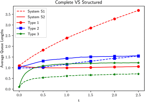
Figure 1 shows that the average queue length of type 1 servers in S1 almost monotonically increases as t increases, which implies that the average queue length of type 1 servers in S1 is unbounded. However, in the system S2, the average queue length of each type of servers is bounded. From this numerical result, we observe that with an appropriately designed graph structure, the performance of the system can be improved. Although we tried to plot the 95% confidence interval (CI) for each point $t=0.5,1.0,1.5,2.0,2.5$, the CI is narrow, and its size is smaller than that of markers in the plot. One reasonable explanation for such a narrow CI is that for large-enough N, the scaled occupancy process ${\mathbf{q}}^N$ is close to the fluid limit q. In other words, the error of the mean-field approximation is quite small, which can be of independent interest. With a similar heterogeneous setting, Allmeier and Gast (2022) show that the error of the mean-field approximation is $O(1/N)$.

6.2. Convergence of Global Occupancy States

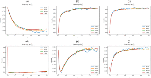
In this experiment, we generate systems by irg(${\mathbf{p}}^1$) and simulate the evolution of systems with size n = 100, 500, 1,000. For each system, we also simulate 100 times and plot the mean trajectories of $q_{m,1}^N$ and $q_{m,2}^N,\hspace{0.17em}m\in \{1,2,3\}$ in Figure 2. Also, we plot the evolution of $q_{m,1}$ and $q_{m,2}$, m = 1, 2, 3, of the limit system. The simulation results show that the evolution of the global occupancy of the Nth system converges to that of the limit system as N goes to infinity. From the simulation result, we find that $q_{1,1}^N$ and especially, $q_{1,2}^N$ decrease very fast when their initial values are large. In other words, when the average queue length of type 1 servers is large, it will decrease very fast. The reason is because of our designed compatibility matrix such that compared with other type servers, type 1 servers are sampled much less often.

6.3. Uniqueness of the Fixed Point of the Limit System

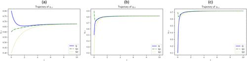
From Theorem 4, we have that for all $\mathbf{q}\in \mathcal{S},\hspace{0.17em}{\lim }_{\to \infty } \overline{\mathbf{q}}(t,{\mathbf{q}}_0)={\mathbf{q}}^{*}$. In order to verify this, we use a simulation of the evolution of $\overline{\mathbf{q}}(t,{\mathbf{q}}_0)$ with different ${\mathbf{q}}_0\in \mathcal{S}$ (i.e., consider the different Q mentioned). We also simulate the system with $Q_1=\left[\begin{array}{ccc}0.4& 0.3& 0.3\\ 0.1& 0.8& 0.1\\ 0.3& 0.6& 0.1\end{array}\right]$ and $Q_2=\left[\begin{array}{ccc}0.6& 0.3& 0.1\\ 0.8& 0.1& 0.1\\ 0.7& 0.2& 0.1\end{array}\right]$. Figure 3 shows that with different $\mathbf{q}\in \mathcal{S},\hspace{0.17em}{\lim }_{t\to \infty }{q}_{m,1}(t)$, m = 1, 2, 3, are the same. If $q_{m,1}$, m = 1, 2, 3 are fixed, then the values of all $q_{m,l},\hspace{0.17em}l\ge 2$, m = 1, 2, 3 are fixed as well by using (5.1). Hence, Figure 3 verifies the uniqueness of the fixed point.

7. Conclusion

In this paper, we model a heterogeneous system as a bipartite graph and investigate how we can impose the data locality to significantly improve the system performance even if the individual task assignment remains oblivious to the service rates. We figure out that if the sequence of systems satisfies the capacity sufficiency, we can always design an appropriate graph structure between dispatchers and servers such that the vanilla JSQ(d) policy achieves maximal throughput and the tail of queue-length distribution decreases doubly exponentially. However, it is worthwhile to mention that although we consider the data locality, which restricts the compatible servers for each dispatcher, our work is not really to investigate the sparsest system. It is an interesting future research direction to see what is the sparsest in which such a compatibility graph can achieve similar favorable properties, like the double-exponential tail decay.

References

- (1995) Parallel randomized load balancing. Proc. 27th Ann. ACM Sympos. Theory Comput. (STOC ’95) (Association for Computing Machinery, New York), 238–247.Google Scholar
- (2022) Mean field and refined mean field approximations for heterogeneous systems: It works! Proc. ACM Measurement Anal. Comput. Systems 6(1):13.Google Scholar
- (2022) Asymptotic optimality of speed-aware JSQ for heterogeneous service systems. Performance Evaluation 157–158(2022):10232.Google Scholar
- (2011) Stability of join the shortest queue networks. Ann. Appl. Probab. 21(4):1568–1625.Google Scholar
- (2019) Supermarket model on graphs. Ann. Appl. Probab. 29(3):1740–1777.Google Scholar
- (2005) Inequalities for eigenvalues of a clamped plate problem. Trans. Amer. Math. Soc. 358(6):2625–2635.Google Scholar
- (2020) Stability of JSQ in queues with general server-job class compatibilities. Queueing Systems 95(3–4):271–279.Google Scholar
- (2009) Markov Processes: Characterization and Convergence (John Wiley & Sons, Hoboken, NJ).Google Scholar
- (1998) On the stability of a partially accessible multi-station queue with state-dependent routing. Queueing Systems 29(1):55–73.Google Scholar
- (2021) Scalable load balancing in the presence of heterogeneous servers. Performance Evaluation 145(2021):102151.Google Scholar
- (2015) The power of two choices on graphs: The pair-approximation is accurate. Performance Evaluation Rev. 43(2):69–71.Google Scholar
- (1998) Probabilistic Methods for Algorithmic Discrete Mathematics, vol. 16 (Springer, Berlin).Google Scholar
- (2021) Throughput and delay optimality of power-of-d choices in inhomogeneous load balancing systems. Oper. Res. Lett. 49(4):616–622.Google Scholar
- (1999) Fast Jackson networks. Ann. Appl. Probab. 9(3):854–870.Google Scholar
- (1996)
Asymptotic behaviour of some interacting particle systems; Mckean–Vlasov and Boltzmann models . Talay D, Tubaro L, eds. Probabilistic Models for Nonlinear Partial Differential Equations, Lecture Notes in Mathematics, vol. 1627 (Springer, Berlin), 42–95.Google Scholar - (1996a) Load balancing and density dependent jump Markov processes. Proc. 37th Conf. Foundations Comput. Sci. (IEEE, Piscataway, NJ), 213–222.Google Scholar
- (1996b) The power of two choices in randomized load balancing. PhD thesis, University of California, Berkeley.Google Scholar
- (2018a) Asymptotically optimal load balancing topologies. Proc. ACM Measurement Anal. Comput. Systems 2(1):14.Google Scholar
- (2018b) Universality of power-of-d load balancing in many-server systems. Stochastic Systems 8(4):265–292.Link, Google Scholar
- (2016) Analysis of randomized Join-the-Shortest-Queue (JSQ) schemes in large heterogeneous processor-sharing systems. IEEE Trans. Control Network Systems 3(2):116–126.Google Scholar
- (2016) Randomized assignment of jobs to servers in heterogeneous clusters of shared servers for low delay. Stochastic Systems 6(1):90–131.Google Scholar
- (2022) Load balancing under strict compatibility constraints. Math. Oper. Res. 48(1):227–256.Google Scholar
- (2005) Optimal routing in output-queued flexible server systems. Probab. Engrg. Inform. Sci. 19(2):141–189.Google Scholar
- (2015) Pull-based load distribution in large-scale heterogeneous service systems. Queueing Systems 80(4):341–361.Google Scholar
- (2017) Pull-based load distribution among heterogeneous parallel servers: The case of multiple routers. Queueing Systems 85(1):31–65.Google Scholar
- (1991) Topics in Propagation of Chaos (Springer, Berlin).Google Scholar
- (2020) Borg: The next generation. Proc. 15th Eur. Conf. Comput. Systems (EuroSys ’20) (Association for Computing Machinery, New York), 1–14.Google Scholar
- (2013) Queueing system topologies with limited flexibility. Proc. ACM SIGMETRICS/Internat. Conf. Measurement and Modeling Comput. Systems (SIGMETRICS ’13) (Association for Computing Machinery, New York), 167–178.Google Scholar
- (2017) Flexible queueing architectures. Oper. Res. 65(5):1398–1413.Link, Google Scholar
- (1998) The effect of increasing routing choice on resource pooling. Probab. Engrg. Inform. Sci. 12(1):109–124.Google Scholar
- (2022) Scalable load balancing in networked systems: A survey of recent advances. SIAM Rev. 64(3):554–622.Google Scholar
- (1996) Queueing system with selection of the shortest of two queues: An asymptotic approach. Problemy Peredachi Informatsii 32(1):20–34.Google Scholar
- (2020) Optimal load balancing with locality constraints. Proc. ACM Measurement Anal. Comput. Systems 4(3):45.Google Scholar