Appointment Requests from Multiple Channels: Characterizing Optimal Set of Appointment Days to Offer with Patient Preferences

1. Introduction

Developed countries have been facing a challenge to balance the trade-off between providing good and timely healthcare services and limiting the associated costs. OECD (2021) shows that the average share of total health expenditure in gross domestic product (GDP) is 8.9% in 2019, while the average share of expenditure on outpatient care in GDP is 2.4% over 35 Organisation for Economic Co-operation and Development (OECD) countries. These figures raise to 16.8% and 7.7% in the United States for total health expenditure and outpatient care expenditure, respectively. This shows that the outpatient care is responsible for 27.4% and 45.7% of the total health expenditure in OECD countries and in the United States, respectively. Hence, the share of outpatient care is quite significant, which suggests that improving outpatient care will considerably enhance the healthcare system and reduce the associated costs.

Appointment scheduling systems constitute a major component of outpatient care. An effective appointment system provides a fast response that will induce short indirect wait times, as well as low levels of cancellation and no-show rates. Consequently, the facility can improve both the overall patient satisfaction and the operations of the system at the same time. Patients usually have preferences for the physician and the date of the appointment. Some studies show that satisfying patient preferences is another factor that decreases cancellation and no-show rates (Bowser et al. 2010). In addition, in many countries, including, but not limited to, Belgium, Germany, Netherlands, Denmark, Switzerland, Austria, Slovenia, Portugal, Turkey, Ireland, Brazil, and the United States, two types of healthcare reimbursement systems exist: private insurance and public insurance (Montagu 2021, OECD 2021). Hence, outpatient clinics in such countries usually serve different patient types who bring different revenues, mostly due to different types of health insurance. In this paper, we develop an appointment scheduling model that aims to help the clinic acknowledge patient preferences and prioritize certain patient types in a way that maximizes the long-run average revenue of the clinic.

Patients usually make an appointment via a call center. However, recently, online appointment scheduling has also been a prominent contact channel, which can be used in different ways: providing real-time appointments online (which we call online appointments), gathering patient requests in a list to contact them later (which we call offline appointments), or a mixture of the two. Many healthcare facilities adopt a mixture of online and offline appointments, such as the Cleveland Clinic, the University of Illinois Hospital, and the Mayo Clinic,¹ whereas offline appointments are frequently used in other industries, such as travel agencies² and repair services.³

From the perspective of appointment scheduling, an online appointment is similar to a call center appointment because in both cases, the patient observes the available days immediately (either through the website or a call center agent) and decides on their appointment day. Here, the clinic can decide only on the available days. However, the offline appointment presents a new challenge and a new opportunity at the same time because the clinic can also choose the patient type to prioritize when contacting the patients in the list.

The university hospital with which we work collects appointment requests through two channels: a call center and a website that provides only offline appointments. The website instructs the patients to enter all the relevant information, in addition to their requests, and collects all requests throughout the day. The list of website requests is shared with the clinic the following morning, upon which the clinic contacts the patients. In every interaction (including the ones via the call center), the clinic offers a patient a set of appointment days. Then, the patient either chooses one of these days or declines the offer. This process is typical in most systems, as the clinics generally quote a set of available days to the patients, and the websites that offer offline appointments always promise to contact the patients within one or two days. Hence, we build our model to represent these features.

Clinics usually plan their appointments over a rolling horizon. This, together with how website patient lists are handled, induces a periodicity to the appointment scheduling process, where every morning, a new day with no prior appointments appears at the end of the rolling horizon, and the schedule of the website patients is finalized. The revenue generated by a patient usually depends on the type of her health insurance, as the hospital fees may vary with respect to the payers. Hence, clinics may assign different priorities to patients based on their insurance status to maximize their expected revenue. This kind of appointment scheduling system is not unique to outpatient care, but can also be observed in other settings, like travel agencies or repair services, as well as in other components of the healthcare system. In particular, our modeling approach and solution techniques are closely related to the literature on ambulatory surgical scheduling, to which we benchmark our contribution in Section 2.

Our first model, Model 1, is a Markov Decision Process (MDP) model that represents both channels and the inherent periodicity of the system. Model 1 aims to determine a dynamic optimal policy, which decides on the set of days to offer to each patient type by accounting for the patient preferences, as well as the revenues. The policy also chooses the patient type to be prioritized in the website list. We show that Model 1 has certain structural properties. Moreover, we adopt the notion of “preferred” from stochastic knapsacks to this setting (Örmeci et al. 2001, Örmeci and Burnetas 2004, Savin et al. 2005) and analyze the conditions for a patient type to be preferred. Surprisingly, generating higher revenues is not sufficient to be preferred, though both types receive the same service, due to the significant effect of patient preferences.

Model 1 serves two purposes: (1) It provides a novel contribution to the literature in the appointment and ambulatory surgical scheduling, as well as in stochastic modeling, as it exhibits valuable structural properties and generates theoretical insights into the optimal sets of choices to offer patients calling in for appointments, while accommodating several features simultaneously: the periodicity of the process due to the rolling time horizon; two channels that collect the appointment requests, one represented by single arrivals and the other by patient lists; and two patient types, who bring different rewards and have different preferences for appointment days, represented by multinomial logit model formulation. (2) Our main motivation is to analyze a constrained MDP model (Model 2), which represents the appointment system of the university hospital with which we work. Model 1 facilitates constructing and understanding Model 2. Moreover, the algorithms developed for Model 1 provide a significant part of the solution methodology built for Model 2.

Model 2 incorporates a service-level requirement in the setting of Model 1. The university hospital with which we work is obliged to accept patients with state insurance, who are similar to Medicare patients in the United States, in addition to patients with private insurance, who generate more revenue. To comply with the government regulations, the hospital has decided to generate at least a certain proportion of the revenues from patients with state insurance. Then, the priority between patient types may change dynamically to satisfy the constraint, depending on the latest figures of the revenues generated by the two patient types. This type of constraints can be seen in different industries as well: a travel agency may be given a sales target for a certain type of vacation, or a bank branch may be required to generate a percentage of the overall sales using a certain service like credits. We characterize the optimal policy of Model 2 as a mixture of two deterministic policies, which will remain valid even when the constraint is altered to another type—for example, the percentage of patients from one type over all patients who receive service should be greater than a given threshold.

Both models are complex and cannot be solved optimally. Hence, our solution methodology focuses on finding good policies of booking limit type, which are easy to implement and quite effective, as shown in the literature; see, for example, Ayvaz and Huh (2010). We first develop a booking limit improvement algorithm (BLIA) to obtain a good solution for Model 1. Then, a constrained problem algorithm (CPA) is proposed for Model 2, based on the characterization of its optimal policy. Repeated use of the BLIA in conjunction with CPA results in our proposed policy, which we call the Mixed Booking Limit (MBL) policy.

Our paper makes the following contributions to the literature.

1. We develop a periodic MDP model that represents an appointment scheduling system, which receives patient requests from a call center and a website providing offline appointments (Model 1). Model 1 determines the optimal set to be offered to each patient and the patient type to be prioritized when contacting the website patients to maximize the long-run average revenue.

2. We analyze the properties of the optimal policy for Model 1: We characterize certain monotonicity properties of the bias function to characterize the structure of the optimal sets (Lemma 1 and Proposition 1). Then, we extend the definition of preferred type to appointment scheduling systems. We derive sufficient conditions for type 1 patients to be preferred and not to be preferred (Proposition 2). We also present sufficient conditions under which the offer-all policy (a commonly used appointment scheduling policy that offers all available days to all patients) is not optimal (Proposition 3). Finally, we show that the bias function has certain monotonicity properties when a booking limit type of policy is adopted (Proposition 4).

3. We extend Model 1 to a constrained MDP model, Model 2, which ensures that the percentage of revenue generated by patients who bring lower rewards should be greater than a fixed threshold. We show that the optimal policy for Model 2 is characterized by a mixture of two deterministic policies, which can differ in, at most, one state (Theorem 1).

4. We propose novel solution methodologies to both Models 1 and 2: Model 1 is solved by BLIA that combines simulation optimization and approximate dynamic programming (ADP). The solution techniques that build up our methodology (explicitly, subgradient method, finite differences estimation algorithm, stochastic gradient algorithm, and ADP imitating the value iteration algorithm using a simulation-based regression) are individually implemented in the literature, yet we combine all of them in a novel way to construct the BLIA. Our solution method for Model 2, CPA, on the other hand, obtains a good randomized policy, as a mixture of two booking limit policies, for Model 2 under the guidance of Theorem 1, where the mixing booking limit policies are generated by the BLIA.

5. We perform a numerical analysis based on the case of a university hospital with which we work. In this context, we describe plausible policies for Model 2 and compare their performance with that of MBL policy. MBL policy generates the highest revenue in almost all cases, by achieving the highest average percent performance of 87.94%, where average percent performance is defined as the percentage of the average revenue that a policy generates relative to the upper bound described in Section 7. When we modify this policy for systems where patients may not show up with certain probabilities, its performance remains similar, with an average percent performance of 84.07%.

The managerial insights generated by the analyses of Model 1 and Model 2 are valuable for both outpatient appointment and ambulatory surgical scheduling. Moreover, the solution methodologies for both models are novel and effective, which can be adopted in different settings that involve large MDP models with or without a constraint, as we discuss in Sections 6 and 8. Hence, we believe that this paper contributes the literature significantly on many fronts.

The organization of the paper is as follows: Section 2 offers a review on the related literature. In Section 3, we introduce Model 1. Section 4 presents the results about the structure of the optimal policy for Model 1. In Section 5, we introduce Model 2 and analyze the structure of its optimal policy. Section 6 develops an algorithm to obtain solutions for both models. In Section 7, we conduct numerical experiments to compare the proposed algorithm with benchmark policies by offering a case study. Finally, we discuss the possible extensions that can be incorporated to our model for future research in Section 8.

2. Literature Review

This section reviews the related papers in appointment scheduling, as well as in assortment planning and revenue management (RM). The analyses of the models and the solution methodologies are related to other subjects as well. We discuss simulation optimization in RM here, while deferring the reviews of others to the corresponding sections.

The literature on appointment scheduling is vast, and there are excellent reviews, such as Çayırlı and Veral (2003), Gupta and Denton (2008), Ahmadi-Javid et al. (2017), and Marynissen and Demeulemeester (2019). We focus on the following features of appointment scheduling: patient types differentiated through their rewards, as well as their preferences for appointment days; different channels that collect the patient requests; rolling horizon; and a constraint on the proportion of rewards collected by the two patient types.

Liu et al. (2010) study an outpatient clinic that schedules appointment requests with the objective of maximizing the long-run average expected net reward. They develop heuristic dynamic policies accounting for the cancellation and no-show behavior of the patients. Studies on patient preferences, on the other hand, consider two settings: Gupta and Wang (2008) and Wang and Gupta (2011) assume that patients inform the clinic about their preferred time slots and physicians, after which the clinic decides to assign the patient to one of his preferences or to reject. In the other setting, the clinic offers the patient a set of time slots (and physicians, in some cases) without knowing the exact patient preferences, and the patient either chooses one of these days or opts for an outside option—for example, Wang and Fung (2015). Liu et al. (2019) seek an answer to an interesting question in the latter setting: is a nonsequential system, where patients are offered a single set of days, or a sequential one, where they are offered multiple sets sequentially, more beneficial? Our model focuses on a nonsequential system, which accounts for appointment requests through both the clinic website (represented by a patient list) and the call center (represented by single arrivals), as opposed to only single arrivals in these studies. Note that modeling website patients and the rolling horizon together also imposes a periodic process that is significantly different than those in the existing literature.

The closest study to our work within the outpatient appointment scheduling literature is by Feldman et al. (2014). They consider a clinic that receives identical patients requesting appointments from a single resource. The patients may cancel their appointments or simply may not show up. They decide dynamically on the set to be offered to the patients, while accounting for the appointment day preferences of the patients. Our model differs from that of Feldman et al. (2014) in several aspects: We consider multiple patient types and a rolling horizon, as opposed to a single patient type and a fixed scheduling horizon. The requests form a stream of single arrivals in Feldman et al. (2014), whereas our model allows both single arrivals via the call center and a patient list through the facility website. Furthermore, our model maximizes the expected average revenue subject to a constraint, whereas the model of Feldman et al. (2014) does not include any constraint. Most importantly, we incorporate a completely different solution methodology.

To the best of our knowledge, Feldman et al. (2014) propose the only model in the literature that considers patient preferences over multiple days. Ahmadi-Javid et al. (2017) also emphasize this fact and the limited work in advance appointment scheduling with patient preferences. Hence, our paper presents the first model in the appointment scheduling literature that considers the rolling horizon, periodicity, multiple priority classes, patient choices, and a service-level constraint for patients generating lower rewards. Furthermore, none of the papers has modeled multiple channels to collect appointment requests as in our paper, which accounts for the demand through both the facility website (requests emerge as a list) and the call center (requests arrive sequentially).

When the appointment slots on the days over the rolling horizon are viewed more generally as resources requested by customers, one can easily see the similarity of our work to the studies in assortment optimization and revenue management. Strauss et al. (2018) review the literature that incorporates customer choice behavior in these two areas. In the area of assortment planning, our work is closest to Bernstein et al. (2015), who optimize the set of products offered to multiple customer segments, while representing the customer choice behavior by the multinomial logit (MNL) model. They assume that all products have the same price, that their inventory level is limited, and that customers arrive sequentially.

In addition to appointment scheduling, the present paper also contributes to advance ambulatory surgical scheduling⁴ with a focus on elective surgeries, whereby each patient is assigned to a future date in the booking horizon. In healthcare systems, there has been a significant shift from inpatient care to ambulatory care, which consists of standardized procedures such as routine surgeries, diagnostic procedures, or imaging (e.g., MRI, ultrasound) (Al-Amin and Housman 2012, Koenig and Gu 2013, Samudra et al. 2016). Hospitals usually allocate available blocks or time slots for an operating room to specific disciplines or specific surgeons. For such hospitals, the surgical scheduling problem consists of three steps: (i) deciding on the amount of time assigned to each surgeon (or each discipline), (ii) developing a block schedule based on the required amount of time for each surgeon, and (iii) assigning individual patients to available time slots or blocks of a specific surgeon (Blake and Donald 2002, Santibáñez et al. 2007, Testi et al. 2007). This paper builds on the third step, which could be classified as an operational decision rather than a strategic decision. In particular, we focus on the standardized ambulatory surgeries of a specific surgeon. Hence, we can plausibly assume that the required surgery duration is fixed and identical for all patients, which are common assumptions in this literature (see, e.g., Gerchak et al. 1996, Gupta 2007, and Min and Yih 2010 for identically distributed surgery durations and Green et al. 2006 and Patrick et al. 2008 for fixed surgery durations).

Within advance surgical scheduling, another categorization is made based on when a surgery date is assigned to a patient. More specifically, in dynamic scheduling, a surgery date is scheduled for a patient immediately during her consultation, whereas in static scheduling, those patients that require a surgery are added to a waiting list, and the patients on the waiting list are contacted and given a date periodically (e.g., at the end of each week or at the beginning of each working day) (Samudra et al. 2016). Although it is being implemented in a substantial number of hospitals, dynamic surgery scheduling has received limited attention in the literature (Samudra et al. 2017), and the majority of the papers investigate the static case (for dynamic surgical scheduling papers, see, e.g., Dexter et al. 1999, 2000, 2001, and Gocgun and Ghate 2012). Patrick et al. (2008), a major study in static surgery scheduling, formulate a model in which available capacity is allocated to the incoming demand of patients with waiting time targets and different priorities. Saure et al. (2012) and Gocgun and Puterman (2014) extend this model to cases when patients request more than one appointment and when the system satisfies certain target dates and tolerances, respectively. All these studies establish priorities over patient types, where patient requests form a waiting list. However, although some of these studies in advance surgery scheduling literature consider target dates and due dates for the surgeries, none of them accounts for patient day preferences explicitly. Furthermore, they either account for static surgery scheduling problems or dynamic surgery scheduling problems (although less frequently), whereas we consider the combination of these two categories. For further information on surgical scheduling, we refer the reader to the review papers of Samudra et al. (2016), Zhu et al. (2019, section 2.3.1), and Abdalkareem et al. 2021, section 4.3).

Finally, we review the papers that use simulation optimization techniques to solve for the RM models. Bertsimas and De Boer (2005) and Van Ryzin and Vulcano (2008b) focus on the RM problem on a flight network. Van Ryzin and Vulcano (2008a) extend this model by taking customer preferences into account. While constructing the general structure of our algorithm, we are inspired by Bertsimas and De Boer (2005), who apply a simulation-based booking limit policy by using an approximation of the value function. We use a parametric approximation, which is different from their approximation methods. Van Ryzin and Vulcano (2008a, b) use stochastic gradient algorithms to improve booking limits for the airline by calculating the sample path gradient vector of the value function using a recursion. Our work is different from these three papers in the following aspects: First, our model allows patient requests to arrive sequentially or emerge as a list, whereas customers arrive only sequentially in their models. Second, we aim to find the optimal set of appointment days to offer without knowing the patient preference, whereas their model accepts or rejects the customer after learning her preference. Lastly, our model has to satisfy a constraint on the proportion of revenues generated by the two patient types. We refer the reader to Amaran et al. (2016) for a detailed review on simulation optimization. We also note that Ahmadi-Javid et al. (2017) offer a section on appointment scheduling papers using this method.

3. The Appointment Scheduling Problem

In this section, we first describe the basic components of the appointment scheduling problem, then present a periodic MDP model, labeled as Model 1.

3.1. Basic Components

3.1.1. Scheduler.

The scheduler controls the appointments of a single care provider, who can examine at most C patients per day, with the aim of maximizing the long-run average revenue. The appointments are given over an N-day rolling horizon. We set $\mathcal{N}=\{0,1,\dots ,N\}$, where day 0 corresponds to today and day n denotes the nth day from today. The scheduler records the number of booked patients on each day over the N-day booking horizon, denoted by $\overrightarrow{x}=(x_0,x_1,\dots ,x_N)$, where x_n denotes the number of booked patients on day n. We define $\overline{S}\subseteq \mathcal{N}$ as the set of all days with available capacity—that is, $\overline{S}=\{n\in \mathcal{N}|x_n<C\}$. For a given set $\mathcal{C}$, we let ${\mathcal{P}}_{\varnothing }(\mathcal{C})$ denote the set that contains all subsets of $\mathcal{C}$, except for the empty set.

We consider a healthcare setting, where ethical issues prohibit rejecting service requests unless the entire horizon is completely booked. Hence, the scheduler offers a set of days $S\in {\mathcal{P}}_{\varnothing }(\overline{S})$ to all patients she contacts, whenever there exists at least a day with available capacity in the booking horizon ($\overline{S}\ne \varnothing$). Patients either select one of the appointment days in the offered set or leave without making an appointment. The empty set is offered only if all slots in the rolling horizon are booked ($\overline{S}=\varnothing$), which occurs rarely for a sufficiently long booking horizon. Therefore, the system rejects a patient only scarcely in this setting. In other settings or in some healthcare settings where the facility can deny access to certain patients (Stanciu 2009, Stanciu et al. 2010), it is possible to reject a service request more often. Our model and solution techniques can handle such situations as well. In fact, some of our results are stronger when the reject decision is allowed in all states.

Finally, we note that the scheduler keeps track of two more components of information in addition to $\overrightarrow{x}$: the list of patients who convey their appointment requests through the website and the time interval within a day, which will be explained below.

3.1.2. Patients.

The single care provider serves two patient types, where a type-i patient brings a reward of r_i with $r_1\ge r_2$. We assume that patients do not cancel their appointments and that they always show up. Hence, collecting the reward at the time of making the appointment is equivalent to collecting it after the service is given when the objective is to maximize the long-run average revenue, and our model is based on the former case. Patients can seek appointments through two different channels: the website or the call center. We assume that call center appointment requests arrive one by one during the working hours, whereas website appointment requests are collected during the day and emerge as a list in the beginning of the following day. The number of website requests has a joint distribution, where $P(y_1,y_2)$ denotes the probability that y₁ type-1 and y₂ type-2 patients request an appointment on a day. We assume that the daily website requests can be at most Y—that is, $y_1+y_2\le Y$ for all (y₁, y₂) with $P(y_1,y_2)>0$.

We model patient preferences based on the multinomial logit model (see Anderson et al. 1992 for detailed information about the MNL model). A type-i patient selects day n over an offered set $S\in {\mathcal{P}}_{\varnothing }(\overline{S})$ with probability $p_{in}(S)$. Letting v_in and $v_i^0$ denote the utility weights of a type-i patient for the option of scheduling an appointment on day n and of leaving the system with no appointment, respectively, we have:

Then, a type-i patient leaves the system without an appointment with probability $p_i^0(S)$:

We note that $p_{in}(S)=0$ if $n\notin S$. Furthermore, in case the entire booking horizon is sold out ($\overline{S}=\varnothing$)—that is, x_n = C for all $n\in \mathcal{N}$—then the empty set is offered, and $p_i^0(\varnothing )=1$.

3.2. Model 1: MDP Model with No Constraint

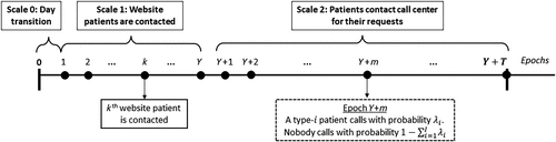
The appointment scheduling system uses a rolling horizon of N days (a total of N + 1 days are considered to include day 0 as today), so that in the beginning of a day, a new day appears in the end of the horizon with no appointments. Each day is planned to have $Y+T+1$ time intervals and three distinct phases, as shown in Figure 1. Hence, the system evolves periodically in multiple time scales, where both the days (denoted by n) and the time intervals within a day (denoted by t) should be taken into account. Jacobson et al. (2003) introduce the so-called Periodically Time-Inhomogeneous Markov Decision Processes (PTMDP) model for such systems, where they identify periods as slow-scale cycles, which consist of shorter time intervals. Two different types of events are labeled as time-homogeneous fast-scale epochs and periodic slow-scale epochs. Our setting is similar, but slightly more complicated, because we have three types of events. This difference requires tracking the time intervals, so that the state should include the time interval as well. Consequently, we build a periodic MDP model, instead of a PTMDP model. However, we adopt the concepts of PTMDPs because they perfectly reflect the properties of the process. We label a working day as a slow-scale cycle, which consists of three scales:

• Scale 0 (t = 0) is a slow-scale epoch in which the system transitions from one day to the next by accounting for the rolling time horizon. Moreover, the scheduler receives the list of patients who asked for appointments via the website throughout the previous day as $\widehat{y}=(y_1,y_2)$. We let w_i denote the number of outstanding type-i website requests and set $\widehat{w}=(w_1,w_2)$. Hence, $\widehat{w}=\widehat{y}$ in scale 0.

• Scale 1 ($1\le t\le Y$) consists of first-order fast-scale epochs in which the scheduler contacts all website patients. She selects a patient type—say, type-j—and contacts a type-j patient in the list to offer a set of days, S. The patient chooses his action according to the MNL model. The scheduler updates the number of outstanding type-i website requests, $\widehat{w}=(w_1,w_2)$, until all patients in the list are contacted—that is, until $\widehat{w}=\widehat{0}$, where $\widehat{0}=(0,0)$. Scale 1 has Y intervals to accommodate all potential contacts due to a website request because the maximum number of website requests is Y.

• Scale 2 ($Y<t\le Y+T$) consists of second-order fast-scale epochs in which the scheduler starts receiving calls from patients who request appointments. We assume that a working day is divided into T identical intervals: The probability that a type-i request arrives in an interval is λ_i, while the probability that nobody calls in an interval is $1-{\lambda }_1-{\lambda }_2$. Upon a call, the scheduler learns the type of the patient, offers a set of days, S, and records his preference. Note that the requests made via the website during the day are not visible to the scheduler in this scale, so the list remains empty—that is, $\widehat{w}=\widehat{0}$—throughout scale 2.

3.2.1. State Space.

The state of the system consists of three components. The first component is the current interval (t); the second component represents the number of website appointment requests waiting to be scheduled (w_i); and the third is the vector that represents the number of already booked appointments (x_n). Hence, the state is:

The state space can now be expressed as:

where $\mathcal{T}=\{0,1,\dots ,Y+T\},\hspace{0.17em}\mathcal{Y}=\{0,1,\dots ,Y\}$ and $\mathcal{C}=\{0,1,\dots ,C\}$. Then, we let $\overline{S}(\mathbf{s})$ be the set of appointment days with available capacity when the state of the system is s—that is, $\overline{S}(\mathbf{s})=\{n\in \mathcal{N}|x_n<C\}$. Finally, letting ${\overrightarrow{e}}_n$ denote a unit vector with N + 1 dimensions, we define the following:

The Transformation (3.3) corresponds to the end of the day when $t=Y+T$, so that the next time interval becomes interval 0 of the following day.

3.2.2. Dynamic Programming Operators.

We start by defining the operator that decides on the set of days to offer when a type-i patient is contacted, noting that $f(\mathbf{s})$ is a generic function defined on the state space $\mathcal{D}$—that is, $f:\mathcal{D}\to \mathbb{R}$:

where

Operator $L_i(S)$ updates the system state for a given set of days offered to a type-i patient, S, whereas operator L_i selects the revenue-maximizing set that will be offered to a type-i patient who is contacted in interval t. The first term in (3.7) accounts for the case when the patient selects day $n\in S$, while the second term corresponds to the possibility that the patient rejects the offer. In scale 1, operator $L_i(S)$ represents the event that a type-i patient in the website list is contacted. Hence, he is removed from the list by the update ${\widehat{w}}_{-i}$ given by (3.4). In scale 2, on the other hand, operator $L_i(S)$ is used when a type-i patient conveys his request via the call center. Because $\widehat{w}=\widehat{0}$ in scale 2, $\widehat{w}$ remains as $\widehat{0}$ after the update (3.4). Now, we introduce the dynamic programming operators for each scale.

• Scale 0: Slow-scale epoch: Let L_s represent the operator for the slow-scale transition (between-day transitions). We define L_s as:

  $$L_{s}f(0,\widehat{0},\overrightarrow{x})={\displaystyle \sum _{y_1=0}^Y{\displaystyle \sum _{y_2=0}^{Y-y_1}P}}(y_1,y_2)f(1,\widehat{y},\overrightarrow{x\prime }),$$(3.8)
  where $\widehat{y}=(y_1,y_2)$ and $\overrightarrow{x\prime }=(x_1,x_2,\dots ,x_N,0)$. Operator L_s has two components: (1) adjusting $\overrightarrow{x}$ to account for the rolling horizon by removing x₀ and adding the $N^{\text{th}}$ day, which has no prior appointments; and (2) bringing the list of website patients, (y₁, y₂), to the state.

• Scale 1: First-order fast-scale epochs: This scale decides on the optimal patient type to be contacted according to an optimal decision rule, ${\mathit{\delta }}^{*}$, given by:

  $${\mathit{\delta }}^{*}(\mathbf{s})=\{\begin{array}{ll}\text{arg}\hspace{0.17em}\text{max}\{L_{i}f(\mathbf{s}):i=1,2\},\hfill & \text{if}\hspace{0.17em}{w}_1>{0 \text{and} w}_2>0,\hfill \\ 1,\hfill & \text{if} w_1>0 \text{and} w_2=0,\hfill \\ 2,\hfill & \text{if} w_1=0 \text{and} w_2>0,\hfill \\ 0,\hfill & \text{if} w_1=0 \text{and} w_2=0,\hfill \end{array}$$(3.9)
  which chooses the patient type that the scheduler should contact first, when the website list includes patients from both types. The optimal set to be offered is determined by $L_{{\mathit{\delta }}^{*}(\mathbf{s})}$, and we set operator $L_{w}f(\mathbf{s})=L_{{\mathit{\delta }}^{*}(\mathbf{s})}f(\mathbf{s})$, where L_i is given by (3.6) for i = 1, 2. Note that ${\mathit{\delta }}^{*}(\mathbf{s})=0$ corresponds to offering an empty set and $p_i^0(\varnothing )=1$, so the state remains the same in (3.7), except for updating the time interval t.

• Scale 2: Second-order fast-scale epochs: Let L_c represent the operator for the second-order fast-scale decisions (call center appointment requests). We define L_c as:

  $$L_{c}f(\mathbf{s})=L_{c}f(t,\widehat{0},\overrightarrow{x})={\displaystyle \sum _{i=1}^2{\lambda }_i}{L}_{i}f(t,\widehat{0},\overrightarrow{x})+\left(1-{\lambda }_1-{\lambda }_2\right)f(\overline{t},\widehat{0},\overrightarrow{x}).$$(3.10)

  The second term in (3.10) corresponds to the event that nobody calls the clinic, whereas the first term is the expectation across all patient types.

Finally, we consider an arbitrary policy ψ and define the corresponding operators for website patients and call center patients as $L_w^{\psi }$ and $L_c^{\psi }$, respectively. Operators $L_w^{\psi }$ and $L_c^{\psi }$ simply use $L_i(S^{\psi })$, where set $S^{\psi }$ is specified by policy ψ. We let ${\delta }^{\psi }(\mathbf{s})$ denote the patient type that policy ψ prioritizes in the website list in state s.

3.2.3. MDP Model.

For an initial state ${\mathbf{s}}_0=\mathbf{s}$, the long-run average revenue per day under an arbitrary policy ψ is

where $H_k({\mathbf{s}}_k)$ is the immediate revenue obtained at decision epoch k in state ${\mathbf{s}}_k$. We solve the following problem to maximize the long-run average revenue over an infinite horizon:where $\mathcal{A}$ is the set of all admissible policies. All patients can reject all the days offered with a positive probability, so the underlying Markov chain is unichain under all policies. Hence, $g^{*}(\mathbf{s})=g$ for all $\mathbf{s}\in S$. Then, there exists an optimal policy, ${\psi }^{*}$, that is deterministic and stationary. Moreover, Model 1 can be represented by the following Bellman equations:that find both the optimal bias function, $h(\mathbf{s})$, and the optimal policy, ${\psi }^{*}$.

The sequel presents the results only for the criterion of the long-run average revenue. However, we prove all the results first for the value functions of the discounted criterion (defined in Online Appendix A), which are then inherited by the bias functions of the long-run average criterion (Puterman 1994).

4. Structural Properties of Model 1

This section explores the structural properties of the optimal policies. We first analyze the optimal sets to offer a type-i patient. Then, we define a preferred patient type and develop sufficient conditions to guarantee its existence. Finally, the structure of the bias function is characterized when the system adopts a booking limit type of policy.

4.1. Structure of Optimal Sets

The structure of the optimal sets in Model 1, given by (3.13), depends on the main trade-off that operator L_i presents, which can be observed by rewriting L_i as follows:

Hence, operator L_i essentially compares the marginal benefit of adding a new type-i patient on day n with a revenue of r_i (denoted by $r_i+f(\overline{t},{\widehat{w}}_{-i},{\overrightarrow{x}}_{+n})$) with that of removing him from the system (denoted by $f(\overline{t},{\widehat{w}}_{-i},\overrightarrow{x})$). To reflect this trade-off, we define the expected marginal benefit of scheduling a type-i patient on day n in state s for scale 1 and 2 separately:

In scale 1, the dependence of the bias function $h(t,\widehat{w},\overrightarrow{x})$ on the time interval t is artificial. Time intervals in scale 1 are defined just to represent all potential decision epochs, so that the actual number of remaining intervals in scale 1 is $w_1+w_2$, not Y – t. Hence, the marginal benefit depends only on $\widehat{w}$ and $\overrightarrow{x}$ in scale 1:

Now, consider scale 2, in which $\widehat{w}=\widehat{0}$. Accordingly, the marginal benefit depends neither on $\widehat{w}$ nor on patient type in scale 2:

It is straightforward to see that if day n is in the optimal set of days to be offered, S, then all days with a higher marginal benefit should also be in set S. Similarly, if a day n is not in set S, then all days with a lower marginal benefit should also be excluded. To utilize this reasoning, we let the sequence of days $(n_1,\dots ,n_{N+1})$ and $(m_1,\dots ,m_{N+1})$ satisfy:

We define sets $S_{ik}^w(\mathbf{s})=\{n_1,n_2,\dots ,n_k\}$ and $S_k^c(\mathbf{s})=\{m_1,m_2,\dots ,m_k\}$ to include the first k days based on the Orders (4.4) and (4.5), respectively. We also let ${\overline{S}}_{ik}^w(\mathbf{s})=S_{ik}^w(\mathbf{s})\cap \overline{S}(\mathbf{s})$ and ${\overline{S}}_k^c(\mathbf{s})=S_k^c(\mathbf{s})\cap \overline{S}(\mathbf{s})$. The next lemma reveals the structure of the optimal sets.

Lemma 1.

1. In scale 1, it is optimal to offer one of the sets ${\overline{S}}_{i1}^w(\mathbf{s}),\hspace{0.17em}{\overline{S}}_{i2}^w(\mathbf{s})$,…, ${\overline{S}}_{i,N+1}^w(\mathbf{s})$ to a type-i patient in state s.

2. In scale 2, it is optimal to offer one of the sets ${\overline{S}}_1^c(\mathbf{s}),\hspace{0.17em}{\overline{S}}_2^c(\mathbf{s})$,…, ${\overline{S}}_{N+1}^c(\mathbf{s})$ to a patient in state s.

Lemma 1 characterizes the potential sets to offer in both scales. The potential sets depend on the patient type in scale 1, whereas they are the same for both patient types in scale 2, due to the definition of ${\mathrm{\Delta }}_n^c(t,\overrightarrow{x})$. Because the only decision of scale 2 is which set to offer, Lemma 1 provides a simple computational basis for finding the optimal decisions in this scale. However, the decisions in scale 1 require not only an optimal set of days to be offered, but also identification of the patient type to be contacted with, ${\mathit{\delta }}^{*}\mathbf{s}$, which Lemma 1 is short of pointing out. The marginal benefit of scheduling a website patient depends on the patient type, as seen in (4.2). Then, choosing the optimal patient type requires comparing the two marginal benefits ${\mathrm{\Delta }}_{1n}^w(\widehat{w},\overrightarrow{x})$ and ${\mathrm{\Delta }}_{2n}^w(\widehat{w},\overrightarrow{x})$. Section 4.2 will shed some light on this issue by presenting sufficient conditions on having preferred patient types. Nevertheless, Lemma 1 specifies the structure of the candidate sets in both scales, which constitutes the building block of the so-called State-Dependent Controlled Scheduling Algorithm, which is a part of the solution methodology.

The analysis of the marginal benefits is very similar to that in Bernstein et al. (2015), who analyze a model on assortment optimization. However, having a rolling horizon means changing the assortment every day by removing one item (today) and adding a new one (day N). The significance of this change reveals itself when the system has a single patient type. Such systems are plausible because sometimes patient types cannot be distinguished at the time of the appointment request, so that all patients bring the same expected revenue and constitute a single patient type. Bernstein et al. (2015) show that the so-called Offer-All (OA) policy, which offers all days with available capacity to all patients, is optimal in systems with single customer type. However, in our case, OA policy is not necessarily optimal due to the rolling horizon. When all days are offered, patients may choose a day later in the horizon, instead of choosing, say, today, which may result in unused capacity. Accordingly, managers should be more cautious with offering all options, even when the system has a single patient type. As a result, we can only prove that the order of the days to be offered coincides with the order of days in real time when n = 2:

Proposition 1.

If the appointment scheduling system has a single patient type that brings a revenue of r and works with a two-day booking horizon, it is optimal to offer either $\{0\}\cap \overline{S}(\mathbf{s})$ or $\{0,1\}\cap \overline{S}(\mathbf{s})$ to an arriving patient.

4.2. Existence of Preferred Patient Types

The concept of preferred types has been introduced in the context of stochastic knapsacks, where different customer types offer different rewards, while requiring different amounts of service. In our problem, both patient types use the same amount of resource. However, the actions (offering a set of days) and their consequences (which depend on patient preferences) are quite complicated when compared with these studies, which assume that the customers can be simply admitted or rejected. Hence, we first need to define a preferred patient type in the context of appointment scheduling:

Definition 1.

Type-i patients are called preferred if (1) it is optimal to schedule type-i website patients first, and (2) it is optimal to offer all days n with $x_n<C$ to type-i patients (both call center and website patients).

Because both patient types request one slot of the physician and type-1 patients offer a higher reward, one can expect that type-1 patients are always preferred. However, this is not always the case, as patient preferences play a crucial role. We consider two simple examples: First assume that both types have the same utility for balking. Moreover, type-1 patients have the same utility for all days in the rolling horizon, whereas type-2 patients have a zero utility for a specific day—say, day k. Hence, day k can be used only by type-1 patients. Then, to fill out the appointments on day k, the optimal policy will probably offer day k to all type-1 patients, while excluding all or some of the other days from the optimal set to maximize the probability that type-1 patients choose day k. In the other example, we assume that the utility of type-1 patients for balking is one ($v_1^0=1$), their utility for day k is two ($v_{1k}=2$), and the utility of all other days is one ($v_{1n}=1$ for all $n\ne k$), while we set the utilities for type 2 as $v_2^0=2$ and $v_{2n}=1$ for all n. Hence, the tendency of type-1 patients to balk is lower than that of type-2 patients. Then, to keep type-2 patients in the system, type-1 patients can be offered only a subset of all available days, especially when there is availability on day k, because they are more likely to choose that day. In both examples, type 1 may not be preferred. The following proposition formalizes this claim and identifies the sufficient conditions under which type-1 patients are preferred and cannot be preferred.

Proposition 2.

1. If

   $$r_2\frac{v_2^0}{v_{2n}}\le r_1\frac{v_1^0}{v_{1n}}\hspace{0.17em} \mathit{\text{for}} \mathit{\text{all}} n\in \mathcal{N},$$(4.6)
   then type-1 patients are preferred.

2. Let ${\widehat{\alpha }}_i,\hspace{0.17em}\widehat{\alpha }$ and ${\widehat{q}}_n$ denote

   $$\begin{array}{ll}\hfill & {\widehat{\alpha }}_i=\frac{{\max }_{n\in \mathcal{N}}{v}_{in}}{v_i^0+{\max }_{n\in \mathcal{N}}{v}_{in}}\hspace{0.17em} \mathit{\text{for}} \mathit{\text{all}} i\in \{1,2\},\hfill \\ \hfill & \widehat{\alpha }=\max \{{\widehat{\alpha }}_1,{\widehat{\alpha }}_2\},\hfill \\ \hfill & {\widehat{q}}_{k\mathcal{\ell }}=\frac{\frac{v_{1\mathcal{\ell }}}{v_1^0+v_{1k}+v_{1\mathcal{\ell }}}·v_1^0/v_{1k}}{\frac{v_{2k}}{v_2^0+v_{2k}}\left(v_2^0/v_{2k}-v_1^0/v_{1k}\right)}\hspace{0.17em} \mathit{\text{for}} \mathit{\text{some}} k,\mathcal{\ell }\in \mathcal{N}.\hfill \end{array}$$

If there exist $k,\mathcal{\ell }\in \mathcal{N}$ with

$$\frac{v_2^0}{v_{2k}}\ge \frac{v_1^0}{v_{1k}},$$(4.7)

and

$$\frac{r_2}{r_1}\ge \frac{1+{\widehat{q}}_{k\mathcal{\ell }}-{(1-\widehat{\alpha })}^{Y(k+1)}{(1-{\lambda }_1{\widehat{\alpha }}_1-{\lambda }_2{\widehat{\alpha }}_2)}^{T(k+1)}}{1+{\widehat{q}}_{k\mathcal{\ell }}},$$(4.8)

then type-1 patients cannot be preferred.

Condition (4.6) in part (1) of Proposition 2 demonstrates that when the revenue from type-1 patients is high enough relative to that from type-2 patients and type-1 patients have higher tendency to balk, then type-1 patients are preferred. On the other hand, part 2 of Proposition 2 establishes that type-1 patients cannot be preferred when (i) type-2 patients have a higher tendency to balk (Condition (4.7)); and (ii) the rewards of the two patient types are close enough and/or the number of time epochs (T) and/or the maximum number of website patients (Y) are too small (Condition (4.8)). Indeed, these conditions ensure that there exists at least one state in which it is not profitable to reserve slots for type-1 patients. More explicitly, it is optimal to schedule type-2 website patients first and offer them all the days with available capacity in at least one state. We note that most of the instances satisfy (4.6) in our numerical experiments, which are based on the data and expert opinion from a university hospital. Therefore, we can conclude that type 1 is preferred in most realistic cases. Accordingly, our solution methodology for Model 1 assumes that type 1 is preferred and finds the booking limits for type 2 only. Hence, the type of the website patients to be contacted next, ${\mathit{\delta }}^{*}\mathbf{s}$, is set to type 1 in scale 1, which significantly speeds up the solution algorithms. Our next result is a negative one, in the sense that we derive sufficient conditions under which OA policy, one of the most commonly used policies in practice, is not optimal.

Proposition 3.

Suppose $T\ge 1$ and set:

$${\zeta }_{in}=\frac{v_{in}}{v_i^0+{\sum }_{k\in \mathcal{N}}{v}_{ik}}\frac{v_i^0}{v_i^0+{\sum }_{k\in \mathcal{N}-\{n\}}{v}_{ik}} \mathit{\text{for}} \mathit{\text{all}} i\in \{1,2\} \mathit{\text{and}} n\in \mathcal{N},$$(4.9)

$${\overline{p}}_{k\mathcal{\ell }}^i=\frac{v_{ik}}{v_i^0+v_{ik}+v_{i\mathcal{\ell }}}\frac{v_i^0}{v_i^0+v_{i\mathcal{\ell }}} \mathit{\text{for}} \mathit{\text{some}} k,\mathcal{\ell }\in \mathcal{N} \mathit{\text{and}} \mathit{\text{for}} \mathit{\text{all}} i\in \{1,2\}.$$(4.10)

Let one of the following conditions hold:

1. There exists an $n\in \mathcal{N}$, which satisfies $\frac{r_2}{r_1}<\frac{{\lambda }_1{\zeta }_{1n}}{1-{\lambda }_2{\zeta }_{2n}}$.

2. $Y\ge C$, and there exist $k,\mathcal{\ell }\in \mathcal{N}$, which satisfies $v_{i\mathcal{\ell }}\ge v_{ik}$ for all $i\in \{1,2\}$ and the following inequality:

   $$\frac{r_2}{r_1}<\frac{(1-{(1-{\lambda }_1{\overline{p}}_{k\mathcal{\ell }}^1-{\lambda }_2{\overline{p}}_{k\mathcal{\ell }}^2)}^{T-1})\frac{{\lambda }_1{\overline{p}}_{k\mathcal{\ell }}^1}{{\lambda }_1{\overline{p}}_{k\mathcal{\ell }}^1+{\lambda }_2{\overline{p}}_{k\mathcal{\ell }}^2}}{1-(1-{(1-{\lambda }_1{\overline{p}}_{k\mathcal{\ell }}^1-{\lambda }_2{\overline{p}}_{k\mathcal{\ell }}^2)}^{T-1})\frac{{\lambda }_2{\overline{p}}_{k\mathcal{\ell }}^2}{{\lambda }_1{\overline{p}}_{k\mathcal{\ell }}^1+{\lambda }_2{\overline{p}}_{k\mathcal{\ell }}^2}}.$$(4.11)

3. $Y<C<Y+T$ and there exist $k,\mathcal{\ell }\in \mathcal{N}$, which satisfies $v_{i\mathcal{\ell }}\ge v_{ik}$ for all $i\in \{1,2\}$ and the following inequality:

   $$\frac{r_2}{r_1}<\frac{(1-{(1-{\lambda }_1{\overline{p}}_{k\mathcal{\ell }}^1-{\lambda }_2{\overline{p}}_{k\mathcal{\ell }}^2)}^{Y+T-C-1})\frac{{\lambda }_1{\overline{p}}_{k\mathcal{\ell }}^1}{{\lambda }_1{\overline{p}}_{k\mathcal{\ell }}^1+{\lambda }_2{\overline{p}}_{k\mathcal{\ell }}^2}}{1-(1-{(1-{\lambda }_1{\overline{p}}_{k\mathcal{\ell }}^1-{\lambda }_2{\overline{p}}_{k\mathcal{\ell }}^2)}^{Y+T-C-1})\frac{{\lambda }_2{\overline{p}}_{k\mathcal{\ell }}^2}{{\lambda }_1{\overline{p}}_{k\mathcal{\ell }}^1+{\lambda }_2{\overline{p}}_{k\mathcal{\ell }}^2}}.$$(4.12)

Then, it is not optimal to follow the OA policy.

We note that ζ_in denotes the probability that a type-i patient prefers day n when all days are offered, while preferring to balk when all days except for day n are offered. On the other hand, ${\overline{p}}_{k\mathcal{\ell }}^i$ denotes the probability that a type-i patient prefers day k when the set $\{k,\mathcal{\ell }\}$ is offered, while preferring to balk when only day $\mathcal{\ell }$ is offered. Hence, we can interpret ζ_in as an expression capturing the preference of a type-i patient for day n relative to all other days, whereas ${\overline{p}}_{k\mathcal{\ell }}^i$ is the one capturing his preference for day k relative to day $\mathcal{\ell }$. The first part of Proposition 3 establishes that the offer-all policy is suboptimal when (i) there exists an appointment day in the booking horizon (say, day n) such that type-2 patients are flexible for day n—that is, they are likely to accept another alternative day if day n is not offered—whereas type-1 patients have a strong preference for it—they have a high tendency to balk, even when all days other than day n is offered (${\zeta }_{1n}$ is high and ${\zeta }_{2n}$ is low); and (ii) the reward and arrival probability of type-1 patients are high relative to those of type-2 patients. On the other hand, provided that there exist two arbitrary days that both type-1 and type-2 patients sort in the same way, according to their utility weights, the second and third parts of Proposition 3 ensure that the offer-all policy is never optimal if the number of decision epochs (T)—or, equivalently, total arrival rate of type-1 and type-2 patients—is sufficiently high (observe in (4.11) and (4.12) that the right-hand side converges to one as T tends to infinity). Note that at least one of these conditions is satisfied in all instances (with a realistic size) of our numerical experiments, suggesting that, in most real cases, OA policy is not optimal.

4.3. Structure of the Bias Functions Under Booking Limit Policies

Appointment scheduling policies in this setting can vary substantially, which poses serious difficulties in analyzing the policy structure. Hence, we restrict our attention to booking limit type of policies, which are known to be effective and easily implementable (Bertsimas and De Boer 2005; Van Ryzin and Vulcano 2008a, b; Ayvaz and Huh 2010; Aydın et al. 2012). In our setting, all appointment slots are shared by all patients, so that whenever a patient makes an appointment, she steals that slot from all other patients. Accordingly, we define the so-called modified booking limit policy⁵ with theft nesting:

Definition 2.

Let $\underset{¯}{n}(\mathbf{s})={\text{arg}\hspace{0.17em}\text{min}}_{n\in \overline{S}(\mathbf{s})} x_n$⁶ and $\mathbf{b}=({\mathbf{b}}_1,{\mathbf{b}}_2)$, where ${\mathbf{b}}_i=(b_{i0},\dots ,b_{in},\dots ,b_{iN})$ is the vector of booking limits for a type-i patient and satisfies $0\le b_{in}\le C$ for all (i, n). Recall that $\overline{S}(\mathbf{s})$ is the set of appointment days with available capacity, and let us define ${\overline{S}}_i^b(\mathbf{s})=\{n\in \mathcal{N}|x_n<b_{in}\}$ and $S_i^{{\varphi }^b}(\mathbf{s})$ as

$$S_i^{{\varphi }^b}(\mathbf{s})=\{\begin{array}{ll}{\overline{S}}_i^b(\mathbf{s}),\hfill & \text{if} {\overline{S}}_i^b(\mathbf{s})\ne \varnothing ,\hfill \\ \left\{\underset{¯}{n}(\mathbf{s})\right\},\hfill & \text{if} {\overline{S}}_i^b(\mathbf{s})=\varnothing \text{and} \overline{S}(\mathbf{s})\ne \varnothing ,\hfill \\ \varnothing ,\hfill & \text{if} \overline{S}(\mathbf{s})=\varnothing .\hfill \end{array}$$

A policy ${\varphi }^b$ denotes a modified booking limit policy if it offers a set of days, $S_i^{{\varphi }^b}(\mathbf{s})$, to a type-i patient in state s. We let $\mathrm{\Phi }$ denote the set of all modified booking limit type policies.

This type of booking limit policy specifies the optimal set of days to be offered to each patient type in all states. More specifically, the scheduler decides on the set of days offered to a patient accounting for both a certain vector of thresholds (b) and the current state of the system—that is, the number of scheduled appointments $(\overrightarrow{x})$. In this respect, for a type-i patient, when there exists at least one day for which the number of scheduled appointments (x_n) is less than the threshold for that day (b_in), the scheduler offers those days that have fewer scheduled patients than the threshold. On the other hand, when the number of scheduled appointments on the entire booking horizon exceeds the thresholds for a type-i patient, the scheduler offers the least crowded day. However, it does not determine which patient type should be contacted first in the website list. We assume that a decision rule $\mathit{\delta }$ to select the patient type to be prioritized is given and set policy $\varphi (\mathit{\delta })$ as the policy composed of the booking limit policy ${\varphi }^b$ and decision rule $\mathit{\delta }$. Then, we can find the best booking limit policy that uses decision rule $\mathit{\delta }$ by solving the equations:

$$h^{\mathit{\delta }}\left(\mathbf{s}\right)+g^{\mathit{\delta }}={\mathcal{L}}^{b,\mathit{\delta }}{h}^{\mathit{\delta }}=\underset{{\varphi }^b\in \mathrm{\Phi }}{\max }\left\{{(L_c^{\varphi (\mathit{\delta })})}^T{(L_w^{\varphi (\mathit{\delta })})}^Y{L}_s{h}^{\mathit{\delta }}(\mathbf{s})\right\},$$(4.13)

where $g^{\mathit{\delta }}$ and $h^{\mathit{\delta }}$ are the corresponding long-run average revenue and the bias function, respectively. When type-i is preferred (denoted by $\mathit{\delta }\equiv \mathit{i}$), type-i website patients are always prioritized, and the booking limits for this type are set to C—that is, $b_{in}=C$ for all n. Characterizing structural properties for the general case is difficult, even for this type of policy. Hence, we consider the system that operates with a booking horizon of two days:

Proposition 4.

Let ${\widehat{\alpha }}_i$ and $\widehat{\alpha }$ denote

$$\begin{array}{ll}\hfill & {\widehat{\alpha }}_i=\frac{{\max }_{n\in \mathcal{N}}{v}_{in}}{v_i^0+{\max }_{n\in \mathcal{N}}{v}_{in}}\hspace{0.17em} \mathit{\text{for}} \mathit{\text{all}} i\in \{1,2\},\hfill \\ \hfill & \widehat{\alpha }=\max \{{\widehat{\alpha }}_1,{\widehat{\alpha }}_2\}.\hfill \end{array}$$

Assume that type-1 patients are preferred—that is, $\mathit{\delta }\equiv \mathbf{1}$—the booking horizon consists of two days (n = 2), and policy ${\varphi }^{b*}$ denotes the optimal modified booking limit type of policy. If

$$\frac{r_2}{r_1}\ge 1-{\left(1-\widehat{\alpha }\right)}^{Y(N+1)}{\left(1-{\lambda }_1{\widehat{\alpha }}_1-{\lambda }_2{\widehat{\alpha }}_2\right)}^{T(N+1)},$$(4.14)

then the bias function $h^{\mathit{i}}(\mathbf{s})$ is componentwise concave and submodular in $\overrightarrow{x}$ for all t and $\widehat{w}$ when policy ${\varphi }^{b*}$ is adopted.

A similar result is obtained when the system has a single patient type (Corollary A1 in Online Appendix B.2). We note that Proposition 2 presents explicit sufficient conditions to guarantee that type 1 is preferred. Hence, Proposition 4 definitely holds under these conditions. We require Condition (4.14) to ensure the submodularity and concavity at the boundaries—that is, when the entire rolling horizon is completely booked. However, the system hits the boundaries very rarely in realistic settings because the rolling horizon is usually long enough. Hence, we observe that the bias function is componentwise concave and submodular, even when Condition (4.14) is not satisfied. Furthermore, when it is possible to offer the empty set in all states, Proposition 4 holds without Condition (4.14).

These results characterize the properties of the optimal solution in stylized settings, but, more importantly, they generate insights into finding the optimal sets when the booking horizon is longer than two days. Indeed, Proposition 4 inspired us to develop an approximation for the bias function, a building block in the solution algorithm in Section 6.1.

5. Model 2: MDP Model with the Constraint

Hospitals, even for-profit hospitals, mainly operate for the public good. Hence, hospital management often needs to balance the benefit of different patient groups. In the university hospital with which we have worked, this balance is represented with the requirement of generating at least a certain fraction of the overall revenue from type-2 patients who bring a lower reward. This prevents the scheduler from reserving too many slots for type-1 patients. Other hospitals may have different requirements, such as having a minimum percentage of patients from each patient type. All such necessities can be addressed with the approach developed in this section. Section 5.1 presents the formulation for the constrained problem, while Section 5.2 analyzes the structure of the corresponding optimal policy.

5.1. Constrained MDP Model

The objective of the constrained problem is to maximize the long-run average revenue per day, subject to the constraint that the fraction of average revenue generated by type-2 patients is more than a user-specified fixed threshold, $\alpha \in (0,1)$. Optimal policies for MDP formulations with constraints are not necessarily deterministic. Instead, they can be characterized as randomized stationary (or Markovian) policies, where a randomized stationary policy, which we denote by $\mathit{\psi }$, maps the set of states into the set of probability distributions over all feasible actions (Puterman 1994).

The underlying Markov chain is still unichain for the constrained problem, so that the long-run average revenue is independent of the initial state under all policies. We let $g_{i,\mathit{\psi }}$ denote the long-run average revenue per day generated by type-i patients under policy $\mathit{\psi }$. Hence, the long-run average revenue per day under policy $\mathit{\psi }$ is:

Then, Model 2 is given by:

We can solve Model 2 by relaxing the constraint with the Lagrangian multiplier $\theta \ge 0$ (Altman 1999):

whereand $g^{\theta }$ is the optimal long-run average revenue for a fixed Lagrangian multiplier θ. The Relaxed Problem (5.3) is reduced to Model 1 (3.11) with the following immediate rewards:due to (5.4). Accordingly, Problem (5.3) can be solved by using Bellman Equations (3.13) with the immediate rewards ${\widehat{r}}_1$ and ${\widehat{r}}_2$ for a given θ. There exists a stationary randomized policy ${\psi }^{*}$ such that:by theorem 12.7 of Altman (1999), and policy ${\psi }^{*}$ is optimal for Model 2 given by (5.2).

5.2. Structural Properties of Model 2

An optimal policy for Model 2 is either deterministic and stationary, which happens when the optimal policy of the original problem (i.e., θ = 0) satisfies the constraint, or a randomized policy that guarantees $\alpha g_{\mathit{\psi }}=g_{2,\mathit{\psi }}$ for $\theta >0$ (formally stated in Lemma A6 in the online appendix). It is difficult, if not impossible, to determine optimal randomized policies for constrained MDP models, unless they have a certain structure. Following Sennott (1993), we can show that the optimal policy for Model 2 is a special kind of randomized policy.

Definition 3.

A mixed policy $\mathit{\psi }=({\psi }_1,{\psi }_2,q)$ is a randomized stationary policy that chooses policy ψ₁ with probability q and policy ψ₂ with probability $1-q$ at each decision epoch, where $0<q\le 1$, and both mixing policies ψ₁ and ψ₂ are stationary and deterministic.

We now show that the optimal policy of Model 2 is a mixed policy using two policies that are identical, except for one state.

Theorem 1.

Let ${\mu }_i={\sum }_{y_1=0}^Y{\sum }_{y_2=0}^{Y-y_1}{y}_{i}P(y_1,y_2)$ denote the expected number of type-i website patients appearing on the list each day. If

$$\frac{r_2\left({\mu }_2+{\lambda }_{2}T\right)}{r_1\left({\mu }_1+{\lambda }_{1}T\right)}\left(\underset{n\in \mathcal{N}}{\min }\frac{v_{2n}/(v_2^0+v_{2n})}{v_{1n}/(v_1^0+v_{1n})}\right)\ge \frac{\alpha }{1-\alpha },$$(5.7)

holds, Model 2 has a feasible solution, and the optimal policy for Model 2 given by (5.2) is a mixed policy $\mathit{\psi }=({\psi }_1,{\psi }_2,q)$. Furthermore, policies ψ₁ and ψ₂ can differ in at most one state.

Condition (5.7) ensures that the fraction of the revenue generated by type-2 patients is more than α, even in the worst-case scenario that the only available day in the booking horizon is always the one that is preferred much less by type-2 patients relative to type-1 patients—that is, the day minimizing $\frac{v_{2n}/(v_2^0+v_{2n})}{v_{1n}/(v_1^0+v_{1n})}$. Obviously, such a condition is quite strong, and, thus, it is highly possible that Model 2 has a feasible solution, even if (5.7) is not satisfied. Indeed, in our numerical experiments, there exists a feasible policy for Model 2, even in the instances that do not satisfy (5.7). Although for the optimal solution of Model 2, we focus on mixed policies, introduced under Definition 3, there also exists an optimal policy, which can be characterized as Bernoulli-modulated simple policy (see Sennott 1993 for details). Under the optimal mixed policy with q < 1, the constraint in (5.2) is satisfied with equality, as shown by Lemma A7 in Online Appendix B.3. To that end, when q < 1, the left-hand side (LHS) of the constraint in (5.2) is slightly less than zero under one of the mixing policies, whereas it is slightly more than zero under the other mixing policy. Moreover, these policies instruct the same actions, except for one state. Theorem 1 forms the basis for CPA (Constrained Problem Algorithm) in Section 6.3.

6. The Solution Methodology

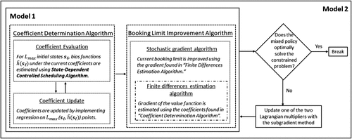
The combinatorial nature of the problem, along with the high-dimensional state, prohibits solving the problem optimally. Hence, we again draw our attention to modified booking limit type policies. This section presents the solution methodology that produces booking limit policies for models 1 and 2. The coefficient determination algorithm (CDA) and the BLIA together find the best modified booking limit policy (or, interchangeably, booking limit policy) for Model 1. The CPA, on the other hand, works with two booking limit policies in each iteration, where one policy produces a positive LHS and the other a negative LHS in the constraint of (5.2). The CPA updates these policies by playing with the Lagrange multiplier θ, until the mixture of the two policies yields to approximately zero in the LHS, upon which it stops with the so-called MBL policy. The structure of the solution methodology is presented in Figure 2. It is worth noting that the CDA and the BLIA together present an alternative solution method for some models proposed in the literature, such as Feldman et al. (2014) and Bernstein et al. (2015). Moreover, solving extensions of these models that include a constraint is possible by implementing CPA in these settings. The three main components—namely, the CDA, the BLIA, and the CPA—are explained in the subsequent sections. The detailed descriptions of all algorithms introduced in this section are presented in Online Appendix C. Throughout this section, we assume that the booking limits, as well as the number of scheduled patients $\overrightarrow{x}$, are continuous to guarantee the convergence of the algorithm.

6.1. Coefficient Determination Algorithm

This section develops an approximation for the bias function and proposes an algorithm to compute this approximation. Because we focus only on booking limit policies, we let $h^{\theta }(\mathbf{s})$ and $g^{\theta }$ denote the bias function and the long-run average revenue, respectively, that correspond to the best-performing booking limit policy, instead of the optimal policy with a slight abuse of notation. Then, we approximate the bias function $h^{\theta }(\mathbf{s})$ by:

which depends only on $\overrightarrow{x}$, but not on t or $\widehat{w}$. The effect of $\widehat{w}$ is absorbed in coefficient K, mainly because $\widehat{w}$ is a realization of the website patients, which has a stationary distribution $P(y_1,y_2)$ that is independent of the system state. The effect of t, on the other hand, is quite low because it refers to a very short time interval.

The optimal policy corresponding to Approximation (6.1) is of booking limit type. Moreover, ${\tilde{h}}^{\theta }(\mathbf{s})$ is componentwise concave and submodular in $\overrightarrow{x}$ for $c_n\le 0$. Remember that the bias function, $h(\mathbf{s})$, is also componentwise concave and submodular in $\overrightarrow{x}$ under booking limit policies for n = 2 by Proposition 4.

For a given set of coefficients $\{K,c_0,c_1\dots ,c_N\}$, we can find the set of days to be offered to a type-i patient using Lemma 1, which depends on the marginal benefits given by (4.2) and (4.3). The estimation of both marginal benefits coincides under Approximation (6.1):

which we denote by ${\tilde{\mathrm{\Delta }}}_n(\overrightarrow{x})$. Ordering the days as ${\tilde{\mathrm{\Delta }}}_{a_{N+1}}(\overrightarrow{x})\le \cdots \le {\tilde{\mathrm{\Delta }}}_{a_2}(\overrightarrow{x})\le {\tilde{\mathrm{\Delta }}}_{a_1}(\overrightarrow{x})$, we define ${\tilde{S}}_m(\mathbf{s})={\tilde{S}}_m(\overrightarrow{x})=\{a_1,a_2,\dots ,a_m\}\cap \overline{S}(\mathbf{s})$. Then, we specify the set of days to be offered to a type-i patient, regardless of whether he contacts through website or call center, in state s:

Hence, when the coefficients of the approximate bias function, ${\tilde{h}}^{\theta }(\mathbf{s})$, is known, we can easily find the optimal sets to be offered to both types.

Now, we consider how coefficients $\{K,c_0,c_1\dots ,c_N\}$ can be estimated. We propose an algorithm that iteratively finds these estimates, where each iteration builds a regression model that relates ${\tilde{h}}^{\theta }(\overrightarrow{x})$ with $\overrightarrow{x}$ using a predetermined number of samples (M). We let $c_n^k$ be the value of the coefficient for x_n and K^k be the value of the constant in iteration k. We set $K^0=0$ as well as $c_n^0=0$ for all n. The initialization sets t = 0 and generates one sample to represent the initial number of appointment requests ($\widehat{w}$), as well as M + 1 samples of the initial number of scheduled appointments ($\{{\overrightarrow{x}}_{\mathcal{\ell }}:\mathcal{\ell }=0,1,\dots ,M\}$), one of which is chosen as the benchmark state (${\mathbf{s}}_0=(0,\widehat{w},{\overrightarrow{x}}_0)$) to estimate the bias function. Hence, in sample $\mathcal{\ell }$, the system starts in state ${\mathbf{s}}_{\mathcal{\ell }}=(0,\widehat{w},{\overrightarrow{x}}_{\mathcal{\ell }})$. Note that the same set of initial states is used in each iteration. Finally, the duration of the simulation is chosen as D days.

Iteration k starts with running the so-called State-Dependent Controlled Scheduling Algorithm (SDCS Algorithm) for M + 1 times, corresponding to M + 1 initial states. This algorithm simulates the system for a given initial state (${\mathbf{s}}_{\mathcal{\ell }}$) over a given number of days D. The algorithm implements decision rule ${\mathit{\delta }}^{\text{sim}}$ to determine the patient type to be contacted in scale 1: If the constraint is satisfied at the current decision epoch, a type-1 patient from the website list is contacted; otherwise, the patient type with the highest ${\widehat{r}}_i$ is chosen. The algorithm determines the set to offer a patient using (6.3) with coefficients $\{K^{k-1},c_0^{k-1},\dots ,c_N^{k-1}\}$. The total reward generated when the system starts in state ${\mathbf{s}}_{\mathcal{\ell }}$ and runs for D days, denoted by $R_k^{\theta }({\mathbf{s}}_{\mathcal{\ell }})$, is recorded at the end of the simulation.

Once simulations for all initial states are completed, the bias function is estimated as ${\tilde{h}}_k^{\theta }({\mathbf{s}}_{\mathcal{\ell }})=R_k^{\theta }({\mathbf{s}}_{\mathcal{\ell }})-R_k^{\theta }({\mathbf{s}}_0)$ for each initial state ${\mathbf{s}}_{\mathcal{\ell }}$. Hence, the simulations in iteration k generate a sample $\{({\mathbf{s}}_{\mathcal{\ell }},{\tilde{h}}_k^{\theta }({\mathbf{s}}_{\mathcal{\ell }})):\mathcal{\ell }=1,\dots ,M\}$, which is used in a regression model to estimate the coefficients $\{K^k,c_0^k,\dots ,c_N^k\}$. If the two sets of coefficients $\{K^{k-1},c_0^{k-1},\dots ,c_N^{k-1}\}$ and $\{K^k,c_0^k,\dots ,c_N^k\}$ are close to each other, the algorithm stops with $\{K^k,c_0^k,\dots ,c_N^k\}$; otherwise, it continues until the maximum number of iterations, I, is reached and stops with $\{K^I,c_0^I,\dots ,c_N^I\}$. The resulting coefficients are used in the BLIA.

6.2. Booking Limit Improvement

This section aims to identify the best booking limit policy that uses decision rule ${\mathit{\delta }}^{\text{sim}}$ (as in the SDCS Algorithm), and the approximations ${\tilde{h}}^{\theta }$ and $\tilde{g}$, with the objective of providing a good solution to the Relaxed Problem (5.3) with a certain Lagrangian multiplier θ. Hence, setting $\varphi =\varphi ({\mathit{\delta }}^{\text{sim}})$, we solve:

Note that the solution of (6.4) presents a good solution to Model 1 where θ = 0.

To find the best booking policy, we propose an algorithm that improves a given booking limit policy $\varphi$ with booking limits b. Our algorithm is based on a classical method, generally known as stochastic approximation, which is widely used in RM; see, for example, Bertsimas and De Boer (2005). This type of algorithms employs a Stochastic Gradient Algorithm (SGA). A generic SGA starts with an initial set of booking limits, ${\mathbf{b}}^0=(b_{in}^0:i=1,2;n\in \mathcal{N})$. Each iteration estimates a sample path gradient and computes a new set of booking limits using the step size and the gradient. It takes the orthogonal projection of the new booking limits onto the feasible set of booking limits, $\mathrm{\Phi }$, when necessary. The algorithm runs for J iterations and returns the latest set of booking limits. Now, we describe the distinct features of our implementation.

We define the indices i₁ and i₂ such that ${\widehat{r}}_{i_2}\le {\widehat{r}}_{i_1}$. We assume that type-i₁ patients are always offered all available days—that is, $b_{i_{1}n}^k=C$ for all $n\in \mathcal{N}$ in all iterations k. Accordingly, the SGA focuses only on the booking limits of type i₂, so we drop i₂ by setting ${\overrightarrow{b}}^k={\overrightarrow{b}}^k(i_2)$. Moreover, the initial booking limits are set to the Expected marginal seat revenue (EMSR) booking limits for type i₂.

Now, we explain the method of estimating the gradients because this is a component of the SGA that varies with respect to the models. We use a Finite Differences Estimation Algorithm (FDEA) to estimate the gradient of the daily average revenue, $g^{\theta }({\overrightarrow{b}}^k)$, with respect to each booking limit, where ${\overrightarrow{b}}^k$ gives the booking limits for type i₂. SGA calls FDEA in iteration k with current booking limits ${\overrightarrow{b}}^k$. We define:

where ${\widehat{\nabla }}_n^k{g}^{\theta }({\overrightarrow{b}}^k)$ denotes the estimate of the marginal improvement in average daily revenue when the booking limit for type-i₂ patients is increased by one on day n.

FDEA generates $\overline{\mathcal{\ell }}$ number of replications, where replication $\mathcal{\ell }$ creates a stream of appointment requests ${\mathbf{d}}^{\mathcal{\ell }}$ for one working day. In each replication, the system starts from the initial state equal to the booking limits—that is, ${\overrightarrow{x}}^0={\overrightarrow{b}}^k=(b_0^k,b_1^k,\dots ,b_N^k)$—so that we can definitely observe the effect of an increase in the booking limits. Replication $\mathcal{\ell }$ simulates the system over $\overline{d}$ days for N + 2 times with $({\overrightarrow{x}}^0,{\mathbf{d}}^{\mathcal{\ell }})$: For ${\overrightarrow{b}}^k$ and ${\overrightarrow{b}}^k+{\overrightarrow{e}}_n$ for $n\in \mathcal{N}$, the average reward for these $\overline{d}$ days is recorded as ${\overline{R}}_{\mathcal{\ell }}^{\theta }({\overrightarrow{b}}^k)$ and ${\overline{R}}_{\mathcal{\ell }}^{\theta }({\overrightarrow{b}}^k+{\overrightarrow{e}}_n)$, whereas the state of the system in the end of $\overline{d}$ days as ${\overrightarrow{x}}^{\varnothing }$ and ${\overrightarrow{x}}^{(n)}$, respectively. Then, the first finite difference for the booking limit $b_n^k$ can be estimated as:

which estimates the improvement through Approximation (6.1) in replication $\mathcal{\ell }$ of FDEA and in iteration k of SGA when $b_n^k$ is increased by one. Thus, in iteration k, the $n^{\text{th}}$ entry of the gradient vector can be estimated by taking the average of ${\widehat{\mathrm{\Delta }}}_n{g}_{\mathcal{\ell }}^{\theta }({\overrightarrow{b}}^k)$ over the randomly generated $\overline{\mathcal{\ell }}$ replications:

We now show that the SGA algorithm using the features described above and in Online Appendix C converges to a local maximum for Model 1. Its proof follows from Van Ryzin and Vulcano (2008b) and Gaivoronski (1988), as shown in Online Appendix B.

Theorem 2.

Consider Model 1, where θ = 0. Then, the SGA converges to a local maximum for the Problem (6.4) in the set of all policies that have type i₁ preferred.

6.3. Constrained Problem Algorithm

The BLIA finds a good solution for Problem (5.3) for a given Lagrangian multiplier θ. However, our main objective is to solve for Model 2 given by (5.2). As opposed to the wide use of SGA, algorithms that solve constrained problems are rather scarce in literature; see, for example, Djonin and Krishnamurthy (2007). Theorem 1 suggests that a mixed policy composed of at most two booking limit policies and a randomization probability $q^{*}$ can provide a good solution to Model 2. This section introduces an algorithm that finds such a randomized policy. The algorithm is based on Formulations (5.3) and (5.6).

The main idea is to find two policies, ${\pi }^{+}$ and ${\pi }^{-}$, with booking limits, ${\overrightarrow{b}}^{+}$ and ${\overrightarrow{b}}^{-}$, where policy ${\pi }^{+}$ generates a strictly positive LHS of the constraint in (5.6), whereas policy ${\pi }^{-}$ generates a strictly negative LHS. Such policies are found by properly changing the Lagrange multiplier, θ. We first solve the problem without the constraint—that is, θ = 0. If the constraint is satisfied, the problem is solved. If not, the LHS is positive, so we have the initial ${\pi }^{+}$. We obtain an initial ${\pi }^{-}$ by solving Problem (5.3) with $\theta =1/\alpha$, so that ${\widehat{r}}_1=0$. Our first goal is to decrease the absolute value of the LHS for one of the policies at each step, until one of them falls in the $\mathcal{E}-$neighborhood of zero or the maximum number of iterations, L, is reached. For this purpose, we update the Lagrange multiplier as follows:

where γ is a positive constant, ν is the corresponding LHS, and ${ϵ}_{\mathcal{\ell }}$ is the step size. This part of the algorithm is computationally intensive because both CDA and BLIA are run for each θ. Hence, we switch to a simpler policy update once one of the policies generates a small enough absolute value for the LHS or the maximum number of iterations, L, is reached. Let policy ${\pi }^{*}$ denote the policy that generates the smallest absolute value for the LHS throughout the iterations of the first part.

In the second part, the algorithm uses the Lagrange multiplier θ and the coefficients $\{c_0,c_1,\dots ,c_N\}$ of policy ${\pi }^{*}$. Initialized with the booking limit of policy ${\pi }^{*}$, the booking limits are updated depending on the gradient of the approximation, given by (6.2), to move the LHS of both policies into the $\mathcal{E}-$neighborhood of zero. Once this is achieved, Bisection Algorithm calculates the randomization probability $q^{*}$ that satisfies the constraint with equality.

7. Numerical Experiments

This section first describes various heuristic policies that are commonly used in practice. Then, we present a case study based on expert opinion and a data set provided by a university hospital. We evaluate the performance of MBL policy, as well as that of other heuristics, in a numerical study built on this case.

7.1. Heuristic Policies

This section introduces the policies used in the numerical experiments. Because of the combinatorial nature of our problem, solving for Models 1 and 2 optimally is not possible in the instances with a realistic size. Therefore, we compare the revenues obtained from the heuristics to the maximum attainable revenue, which is labeled as Upper Bound (UB). We find this bound similarly to Wang and Gupta (2011): the UB is the objective function value of a linear program, which solves Model 2 without the integer constraints and by allowing offering the empty set⁷ when the sequences of appointment requests and day selection outcomes are known over the planning horizon, where these sequences are generated through simulation.

In addition to MBL policy, we introduce three simple heuristic policies that are used in practice:

• Straw Policy (SP) offers the first two days with available capacity.

• Offer-All Policy (OA) offers all the days in the booking horizon with available capacity.

• EMSR Policy (EMSR) implements the EMSR booking limits for Model 1 in the following modified way: The days for which the number of scheduled appointments (x_n) is less than the EMSR threshold are offered. If no such day exists—that is, if the number of scheduled appointments on the entire booking horizon exceeds the corresponding EMSR thresholds—the least crowded day is offered.

These policies satisfy the constraint by using a randomized policy that mixes the heuristic with the policy that always offers only the least crowded day to type-1 patients, which is found by the Bisection Algorithm.

7.2. A Case Study

We analyze the appointment scheduling process in the dermatology clinic of a private university hospital. The hospital receives two types of patients: those with private insurance constitute type-1 patients, whereas those with Social Security Institution (SSI) insurance are labeled as type-2 patients. At the time of our interaction, the insurance type of the patient is revealed before a set of appointment days is offered, and the offer-all policy is implemented by the clinic scheduler.

7.2.1. Data Analysis and Experimental Setup.

The clinic employs multiple physicians, but we focus on the appointment schedule of a specific physician—say, Physician A. The hospital shared a data set, which includes the type of the patient, the contact channel, the physician with which the patient consulted, and the corresponding appointment date for all requests over a month. We estimate the ratio of type-i patients, as well as the ratio of call center patients from this set. Hence, we set ${\mathrm{\Lambda }}_2=2{\mathrm{\Lambda }}_1$ and p_c = 85% in the base instance. We assume that the number of type-i website requests is truncated Poisson with rate ${\mathrm{\Lambda }}_i(1-p_c)$ and truncation parameter $2{\mathrm{\Lambda }}_i(1-p_c)$. We set the number of time intervals for calls over a day, T, to the smallest number that limits the probability of receiving more than one call in a time interval by 1%. Accordingly, T depends on Λ and p_c. The other parameters of the base instance are specified according to the expert opinion obtained from the hospital. Table 1 presents the parameter values used in the numerical experiments and labels the base case parameters by ^b and the small instance parameters by ${}^{\diamond }$.

Table 1. Values of Parameters

The number of available appointments is 13 per day. The hospital aims to collect at least 52.6% of the revenue from SSI patients—that is, $\alpha =0.526$. At the time of the data collection, the hospital was relatively young, and the daily number of appointments was quite low. However, now, the hospital is well known in the community and attracts many patients. Accordingly, we set the total arrival rates as ${\mathrm{\Lambda }}_1=7$ and ${\mathrm{\Lambda }}_2=14$ in our base instance.

We consider three sets of utility weights to represent patient preferences. The base case, denoted by scenario 0, aims to reflect the call center experience, which shows that all patients have higher preference for days 0 and 1. Consequently, we set $v_{i0}^0=v_{i1}^0=5$. The utility weight of type-1 patients decreases sharply for the remaining days, as their private insurance provides them the flexibility of looking for alternative healthcare providers, represented by setting $v_1^{00}=1$. Such alternatives are scarce for the SSI patients, indicated by $v_2^{00}=0.3$. Accordingly, type-2 patients have high utility for the other days as well, and we set $v_{22}^0=5$ and $v_{2n}^0=3$ for $n=3,\dots ,6$. These are also consistent with the socioeconomic background of the patient types. In this setting, type-1 patients are inflexible, with a strict preference for days 0 and 1, whereas type-2 patients are flexible, with a high preference for accessing service throughout the rolling horizon.

In scenario 1, type 1 is still inflexible with the same utility weights as in the base case, whereas type-2 patients have a clear preference for days 2–6, when compared with the earlier days or leaving the system. Even though it may seem that preferences of the two types are complementary, this scenario represents one of the more competitive cases: type-2 patients are likely to fill out the appointments for later days, leaving no room for type-1 patients when they call in for appointments on day 0 or 1 due to the rolling horizon. Finally, scenario 2 sets the same utility weights to both patient types. In this case, day 1 is preferred the most with a weight of six, after which the weights decrease by one every day, while alternative healthcare providers are also viable and the preference for day 0 is rather low. The other parameters we experiment with are percentage of call center patients (p_c), type-2 reward (r₂), minimum proportion of the revenue generated by type-2 patients (α), and total arrival rate of patients (${\mathrm{\Lambda }}_1,{\mathrm{\Lambda }}_2$), as shown in Table 1.

7.2.2. Performance Analysis of Policies.

Our numerical experiments compare the performance of all policies to the upper bound. To understand the quality of this upper bound, we created small-scale instances that can be solved optimally, by setting the duration of the rolling horizon to two and the number of slots per day to four and updating the arrival rates and the utility weights accordingly, while keeping the rest of the parameters the same as in the general setting. As a result, we construct 12 ($2\times 3\times 2$) small-scale instances by changing type-2 reward (r₂), arrival rates $({\mathrm{\Lambda }}_1,{\mathrm{\Lambda }}_2)$, and percentage of call center requests (p_c) (see the parameters indicated by “${}^{\diamond }$” in Table 1). We solve all these instances optimally and run 100 replications under MBL policy for 90 days with a warm-up period of 10 days. The average percentage of daily revenue under MBL policy relative to the optimal revenue is 98.73%. Furthermore, average percentage of daily revenue under MBL policy relative to the upper bound is 96.01%. This shows that MBL policy performs very closely to the optimal policy, whereas the upper bound is rather loose.

Now, we evaluate the performance of policies in the base case and investigate the effects of the changes with one-way sensitivity analysis: The values of the parameters, p_c, u, α, $\widehat{r},\hspace{0.17em}({\mathrm{\Lambda }}_1,{\mathrm{\Lambda }}_2)$ (given in Table 1), are changed one by one in the base case. Hence, we create a total of 10 instances, as shown in Table 2. For each instance, we run the simulation for 90 days with a warm-up period of 10 days. We use the same sample path while simulating all policies and conduct 30 replications. We implemented these experiments on a computer with a 2.60-GHz CPU and 8 GB of RAM. We used MATLAB 9.11.0 under the Windows 10 operating system to run the codes. The average CPU times for SP, OA, EMSR, and MBL policies are 30.56, 40.06, 36.08, and 643.89 seconds, respectively. By testing several other algorithm implementation parameters, we decided to run our experiments with the ones provided in Online Appendix C, which we believe maintains the trade-off between the computation time and the quality of the solution in the best manner concerning our criteria. However, one can further reduce the computation time (possibly) at the expense of the solution quality by changing these parameters—for example, by decreasing the precision (higher $\mathcal{E}$) in the Constrained Problem Algorithm or by decreasing the maximum number of iterations in the Stochastic Gradient Algorithm (lower J).

Table 2. Performance of Policies with Respect to the Upper Bound

Table 2 shows the percentage of the average revenue for each policy relative to the upper bound, which we refer to as percent performance. The upper bounds are obtained through simulations, so depict some randomness. Still, they are insensitive to the model parameters (ranging between 2,228 and 2,410), except for α and r₂, which significantly decrease and increase the UBs, respectively. The average daily revenue under MBL policy is 87.94% of the upper bound. We observe that MBL performs significantly better than all the simple heuristics with a significance level of 5%, in all instances except for one: in this case, where $\alpha =72.6\%$, OA performs better than MBL on the average, but the two policies practically perform the same without a statistical difference.

Both SP and OA, which do not consider any of the RM issues, perform badly, with an average of 79.67% and 81.48%, respectively. The classical RM tool, EMSR, improves them with an average of 83.29%, which is still considerably worse than MBL. The difference between the performance of EMSR and MBL can be accounted for by the two distinguishing features of our problem: the patient preferences and the constraint on the percentage of revenues generated from type 2. When these features are ignored, the revenue loss can be quite substantial because even the small improvements in the daily revenues result in large profits for the yearly revenue of the hospital.

When the effects of parameters are considered, we observe that the performance of the heuristics with respect to the UB improves with α; in particular, all heuristics perform the worst and the best when the constraint that favors type-2 patients is at the least demanding value ($\alpha =32.6\%$) and at the most demanding value ($\alpha =72.6\%$), respectively. This is due to the worsening performance of the UB with respect to α—that is, all policies perform equally badly in more demanding environments. Another interesting observation is on the effect of the system load: The performances of all policies decrease substantially with the load due to the following rationale: As the load increases, the number of scheduled type-2 patients increases under all policies because the facility offers all patients a nonempty set of appointment days—as long as the entire rolling horizon is not completely booked—and type-2 patients are flexible enough so that they usually accept one of the offered appointment days, rather than balking. On the other hand, as the load becomes higher, the number of type-1 patients who prefer balking increases because they have strict preferences for days 0 and 1, which are already occupied by type-2 patients, and, thus, in most cases, they leave the system without making an appointment. We note that the UB does not change much with the load because the load is already high in the base case. In other words, increasing the arrival rates does not offer a high potential for improvement. In conclusion, MBL policy is the best-performing policy in all instances, and we expect it to generate high revenues in a wide range of parameter settings.

7.2.3. Numerical Experiments with No-Shows.

In healthcare systems, it is quite common to observe that patients do not show up for their appointments (Çayırlı and Veral 2003). Accordingly, this section focuses on systems where patients may not show up for their appointments with a certain probability. More specifically, we aim to assess the performance of a “modified” MBL policy in such systems. Our approach is similar to the previous section, as the same heuristic policies are evaluated with respect to an upper bound found by solving an appropriate linear program. We should note that no-shows bring an additional complication because hospitals need to schedule more patients than the daily slot capacity to protect themselves from working under capacity. This implementation may result in physician overtime. Hence, the objective function in this case should account for the expected overtime cost as well.

We let δ_i denote the probability that a type-i patient does not show up. MBL and EMSR can be easily modified by increasing the booking limits—say, b_ij—considering the effective arrival rate—that is, ${\mathrm{\Lambda }}_1(1-{\delta }_1)+{\mathrm{\Lambda }}_2(1-{\delta }_2)$—versus total arrival rate, Λ:

where the function $[a]$ returns the nearest integer to any real number a. We set the overtime cost, c_o, as 1.5 times of the average revenue:

In this setting, it is better to reserve the overtime capacity to type-1 patients because the revenue obtained from type-2 patients is much lower than the overtime cost.

We experiment with three sets of $({\delta }_1,{\delta }_2)$, which are $({\delta }_1,{\delta }_2)=(0.25,0.025),\hspace{0.17em}({\delta }_1,{\delta }_2)=(0.1,0.1)$, and $({\delta }_1,{\delta }_2)=(0.05,0.125)$. Noting that in our experiments, we set the relationship between the total arrival rates of type-1 and type-2 patients as ${\mathrm{\Lambda }}_2=2{\mathrm{\Lambda }}_1$ (recall Section 7.2.1 for a detailed explanation about the parameter setting), for all these three sets of $({\delta }_1,{\delta }_2)$, the weighted average no-show rate, denoted by $\overline{\delta }$, is equal to 0.1—that is, $\overline{\delta }=({\delta }_1{\mathrm{\Lambda }}_1+{\delta }_2{\mathrm{\Lambda }}_2)/\mathrm{\Lambda }=0.1$. Furthermore, to keep the system load the same as that in the experiments conducted in Section 7.2.2 without allowing no-shows, we set the total arrival rates as ${\mathrm{\Lambda }}_1=7/(1-\overline{\delta })$ and ${\mathrm{\Lambda }}_2=14/(1-\overline{\delta })$. Table 3 presents the results for $({\delta }_1,{\delta }_2)=(0.25,0.025)$, as this reflects the patient behavior the best, according to the expert opinion. The results for $({\delta }_1,{\delta }_2)=(0.1,0.1)$ and $({\delta }_1,{\delta }_2)=(0.05,0.125)$ are placed in Online Appendix D.1. Table 3 shows that the relative performance of heuristic policies with respect to each other is similar to the previous case. In particular, MBL still performs significantly better than all other heuristics in all cases, except for policy EMSR when $\alpha =72.6\%$. Hence, we can conclude that MBL is the best heuristic policy. The average performance of MBL with respect to the upper bound is 84.07%, which is close to its previous value, 87.94%, suggesting that the relative performance of MBL to the upper bound, as well as other policies, does not change too much in systems with no-shows. This also shows that the methodology used to compute MBL policy is robust, as it performs well, even when the underlying modeling assumptions are changed. Finally, we note that the average CPU times for SP, OA, EMSR, and MBL policies are 34.79, 31.87, 53.20, and 819.02 seconds, respectively.

Table 3. Performance of Policies with Respect to the Upper Bound When $({\delta }_1,{\delta }_2)=(0.25,0.025)$

8. Conclusion

We consider the appointment scheduling problem of a physician who receives two types of patients, differentiated by their revenues and utility weights for each appointment day. Furthermore, appointment requests may come via the website of the facility or the call center. We formulate this system as a periodic Markov decision process, denoted by Model 1, to maximize the expected average revenue by offering each patient a set of appointment days. Patients either select one of the appointment days in this set or reject the offer. We derive certain structural properties of Model 1, which provide new managerial insights for the appointment scheduling literature. In particular, we define “preferred patient types.” Interestingly, the type that generates higher rewards is not necessarily the preferred type—although both patient types require the same amount of service—that is, one appointment slot. This demonstrates that patient preferences play a crucial role in the preferred type. Moreover, we prove that the offer-all policy, a commonly used policy in healthcare systems, might be sometimes suboptimal. Our numerical results show further that implementing the offer-all policy can result in a severe revenue loss compared with the MBL policy in different settings, except when the appointment day preferences of the two patient types are not competitive (u = 2). We extend Model 1 to satisfy the constraint that the fraction of revenue generated by patients who bring a lower reward is above a threshold. The optimal policy of the latter model is a mixed policy obtained by randomizing between at most two deterministic policies. By utilizing this structure of the optimal policy, we develop an algorithm based on the simulation optimization.

We compare the performance of MBL policy, obtained by the proposed algorithms, with benchmark policies, including widely used policies, such as offer-all and EMSR, in a set of numerical experiments. The setting for the experiments is based on the data and expert opinion provided by a university hospital. We observe that MBL policy carefully selects the days to be offered to each patient, so that some slots are preserved for higher-priority patients. Hence, its performance is uniformly good over all experiments, practically obtaining the highest average revenue in all cases. These observations suggest that this methodology can be effectively implemented to solve other models in settings varying from appointment scheduling (e.g., Feldman et al. 2014) to assortment optimization (e.g., Bernstein et al. 2015). We note that the proposed methodology consists of different modules, which can be used separately in an effective way as well. For example, the simple EMSR policy considered in this paper can be extended to a policy composed of two different EMSR booking limits, by implementing the Constrained Problem Algorithm.

The setting we consider has some limitations: First, we do not consider the no-show and the cancellation behavior of the patients, but our model can be easily extended to represent these features. We illustrate this by modifying the MBL for systems where patients may not show up for their appointments. Our numerical experiments show that the performance of the modified MBL is close to that of the MBL in systems without no shows. Accordingly, we conclude that the methodology used to compute the MBL is quite robust with respect to different characteristics of the systems. Second, we assume that the duration of each appointment is fixed. Instead, a random service time can be introduced in the model. Another limitation of our formulation is to consider only the day preferences of patients, while ignoring the patient preferences for the appointment time. Indeed, this is a common assumption in both appointment and surgical scheduling literature (see, e.g., Patrick et al. 2008, Feldman et al. 2014, Parizi and Ghate 2016) because capturing both the day and time preferences poses a difficult combinatorial optimization problem with a very high-dimensional state. We present an extension of our formulation that additionally incorporates patients’ appointment time preferences over a day in Online Appendix D.2. We expect that our theoretical results will continue to hold in this case. However, it cannot escape the problems due to high dimensionality, especially for realistic scenarios. Finally, it is possible to schedule multiple physicians within the same department. In this case, patients who are not offered an appointment on their preferred day may switch to another physician who is available on that particular day. These extensions may be interesting topics for future research.

References

- (2021) Healthcare scheduling in optimization context: A review. Health Tech. 11:445–469.Google Scholar
- (2017) Outpatient appointment systems in healthcare: A review of optimization studies. Eur. J. Oper. Res. 258(1):3–34.Google Scholar
- (2012) Ambulatory surgery center and general hospital competition: Entry decisions and strategic choices. Health Care Management Rev. 37(3):223–234.Google Scholar
- (1999) Constrained Markov Decision Processes, vol. 7 (CRC Press, Boca Raton, FL).Google Scholar
- (2016) Simulation optimization: A review of algorithms and applications. Ann. Oper. Res. 240(1):351–380.Google Scholar
- (1992) Discrete Choice Theory of Product Differentiation (MIT Press, Cambridge, MA).Google Scholar
- (2012) Single-leg airline revenue management with overbooking. Transportation Sci. 47(4):560–583.Link, Google Scholar
- (2010) Allocation of hospital capacity to multiple types of patients. J. Revenue Pricing Management 9(5):386–398.Google Scholar
- (2015) Dynamic assortment customization with limited inventories. Manufacturing Service Oper. Management 17(4):538–553.Link, Google Scholar
- (2005) Simulation-based booking limits for airline revenue management. Oper. Res. 53(1):90–106.Link, Google Scholar
- (2002) Mount Sinai Hospital uses integer programming to allocate operating room time. Interfaces 32(2):63–73.Link, Google Scholar
- (2010) A systematic review of the relationship of diabetes mellitus, depression, and missed appointments in a low-income uninsured population. Arch. Psychiatr. Nurs. 24(5):317–329.Google Scholar
- (2003) Outpatient scheduling in healthcare: A review of literature. Production Oper. Management 12(4):519–549.Google Scholar
- (2001) The impact on revenue of increasing patient volume at surgical suites with relatively high operating room utilization. Anesthesia Analgesia 92(5):1215–1221.Google Scholar
- (2000) Scheduling surgical cases into overflow block time—Computer simulation of the effects of scheduling strategies on operating room labor costs. Anesthesia Analgesia 90(4):980–988.Google Scholar
- (1999) An operating room scheduling strategy to maximize the use of operating room block time: Computer simulation of patient scheduling and survey of patients’ preferences for surgical waiting time. Anesthesia Analgesia 89(1):7–20.Google Scholar
- Djonin DV, Krishnamurthy V (2007) Structural results on optimal transmission scheduling over dynamical fading channels: A constrained Markov decision process approach. Agrawal P, Fleming PJ, Zhang L, Andrews DM, Yin G, eds. Wireless Communications, The IMA Volumes in Mathematics and its Applications (Springer, New York), 75–98.Google Scholar
- (2014) Appointment scheduling under patient preference and no-show behavior. Oper. Res. 62(4):794–811.Link, Google Scholar
- Gaivoronski A (1988) Implementation of stochastic quasigradient methods. Ermoliev YM, Wets R-B, eds. Numerical Techniques for Stochastic Optimization (Springer-Verlag, Berlin, Heidelberg), 313–352.Google Scholar
- (1996) Reservation planning for elective surgery under uncertain demand for emergency surgery. Management Sci. 42(3):321–334.Link, Google Scholar
- (2012) Lagrangian relaxation and constraint generation for allocation and advanced scheduling. Comput. Oper. Res. 39(10):2323–2336.Google Scholar
- (2014) Dynamic scheduling with due dates and time windows: An application to chemotherapy patient appointment booking. Health Care Management Sci. 17(1):60–76.Google Scholar
- (2006) Managing patient service in a diagnostic medical facility. Oper. Res. 54(1):11–25.Link, Google Scholar
- (2007) Surgical suites’ operations management. Production Oper. Management 16(6):689–700.Google Scholar
- (2008) Appointment scheduling in healthcare: Challenges and opportunities. IIE Trans. 40(9):800–819.Google Scholar
- (2008) Revenue management for a primary-care clinic in the presence of patient choice. Oper. Res. 56(3):576–592.Link, Google Scholar
- (2003) Markov decision processes with slow scale periodic decisions. Math. Oper. Res. 28(4):777–800.Link, Google Scholar
- (2013) Growth of ambulatory surgical centers, surgery volume, and savings to Medicare. Amer. J. Gastroenterology 108(1):10–15.Google Scholar
- (2019) Managing appointment booking under customer choices. Management Sci. 65(9):4280–4298.Link, Google Scholar
- (2010) Dynamic scheduling of outpatient appointments under patient no-shows and cancellations. Manufacturing Service Oper. Management 12(2):347–364.Link, Google Scholar
- (2019) Literature review on multi-appointment scheduling problems in hospitals. Eur. J. Oper. Res. 272(2):407–419.Google Scholar
- (2010) An elective surgery scheduling problem considering patient priority. Comput. Oper. Res. 37(6):1091–1099.Google Scholar
- (2021) The provision of private healthcare services in European countries: Recent data and lessons for universal health coverage in other settings. Frontiers Public Health 9:636750.Google Scholar
OECD (2021) Health expenditure and financing. Accessed October 5, 2021, https://stats.oecd.org/index.aspx?datasetcode=sha.Google Scholar- (2004) Admission with batch arrivals. Oper. Res. Lett. 32:448–454.Google Scholar
- (2001) Admission policies for a two class loss system. Stochastic Models 17(4):513–539.Google Scholar
- (2016) Multi-class, multi-resource advance scheduling with no-shows, cancellations and overbooking. Comput. Oper. Res. 67:90–101.Google Scholar
- (2008) Dynamic multipriority patient scheduling for a diagnostic resource. Oper. Res. 56(6):1507–1525.Link, Google Scholar
- (1994) Markov Decision Processes (John Wiley & Sons, Hoboken, NJ).Google Scholar
- (2017) Due time driven surgery scheduling. Health Care Management Sci. 20:326–352.Google Scholar
- (2016) Scheduling operating rooms: Achievements, challenges and pitfalls. J. Scheduling 19:493–525.Google Scholar
- (2007) Surgical block scheduling in a system of hospitals: An application to resource and wait list management in a British Columbia health authority. Health Care Management Sci. 10:269–282.Google Scholar
- (2012) Dynamic multi-appointment patient scheduling for radiation therapy. Eur. J. Oper. Res. 223(2):573–584.Google Scholar
- (2005) Capacity management in rental businesses with two customer bases. Oper. Res. 53(4):617–631.Link, Google Scholar
- (1993) Constrained average cost Markov decision chains. Probab. Engrg. Inform. Sci. 7(1):69–83.Google Scholar
- (2009) Applications of revenue management in healthcare. Unpublished doctoral dissertation, University of Pittsburgh, Pittsburgh.Google Scholar
- Stanciu A, Vargas L, May J (2010) A revenue management approach for managing operating room capacity. Johansson B, Jain S, Montoya-Torres J, Hugan J, Yücesan E, eds. Proc. 2010 Winter Simulation Conf. (IEEE, Piscataway, NJ), 2444–2454.Google Scholar
- (2018) A review of choice-based revenue management: Theory and methods. Eur. J. Oper. Res. 271(2):375–387.Google Scholar
- Testi A, Tanfani E, Torre G (2007) A three-phase approach for operating theatre schedules. Health Care Management Sci. 10:163–172.Google Scholar
- (2008a) Computing virtual nesting controls for network revenue management under customer choice behavior. Manufacturing Service Oper. Management 10(3):448–467.Link, Google Scholar
- (2008b) Simulation-based optimization of virtual nesting controls for network revenue management. Oper. Res. 56(4):865–880.Link, Google Scholar
- (2015) Dynamic appointment scheduling with patient preferences and choices. Indust. Management Data Systems 115(4):700–717.Google Scholar
- (2011) Adaptive appointment systems with patient preferences. Manufacturing Service Oper. Management 13(3):373–389.Link, Google Scholar
- (2019) Operating room planning and surgical case scheduling: A review of literature. J. Comb. Optim. 37:757–805.Google Scholar