Ergodic Control of Bipartite Matching Queues with Class Change and Matching Failure
Abstract
Motivated by transplant applications, we study a bipartite matching queue with multiclass customers and multitype resources. Customers may change their classes or abandon the system while waiting in queue, and they may decline the offered resource units which results in matching failure. We are interested in designing efficient instantaneous matching policies that allocate resources upon arrival to waiting customers. Our objective is bicriteria and formulated as a cost functional that linearly combines the long-run average expected reward due to successful matches and the long-run average expected cost from customer waiting and abandonment. We first develop a stability condition on the class change and abandonment rates, which requires at least one customer queue with abandonment and that any queue without abandonment have a class transition path to a queue with abandonment. Under this condition, we construct a simple linear program, referred to as the fluid control problem (FCP), which serves as a lower bound for the original stochastic control problem under any admissible policy. We then propose a randomized matching policy based on the solution of the FCP and show that the proposed policy is asymptotically optimal under both the long-run average and ergodic cost criteria. In addition, we apply our method to study two X matching models with two customer classes and two resource types to provide insights on how the class change and matching failure impact the optimal policies.
1. Introduction
1.1. Motivation and Problem Statement
Although matching supply and demand has been a long-lasting problem (Roth and Sotomayor 1992), the advent and diffusion of online platform applications have spurred notable research in the operations community (Chen et al. 2020). Demand and supply are usually heterogeneous belonging to different classes/types. In many applications such as organ transplant matching systems and ridesharing systems, demand is from impatient customers and those customers may abandon the system if they wait too long, and supply should be allocated to waiting demand quickly. In addition, customers may change classes while waiting in the system. For example, in organ transplant and other healthcare applications, patients’ classes can change because of their health deterioration or improvement, and in service systems, customers can switch between regular and VIP classes. Motivated by these applications, we study a multiclass bipartite matching queue with class change, and focus on instantaneous matching policies that assign each supply unit upon arrival to waiting customers.
In the queueing system we consider, customers belonging to different classes arrive to one side of the system according to Poisson processes, join their class-dependent queues, and wait in queue to be matched with resources. On the other side, resources with different types arrive according to Poisson processes and are allocated to the waiting customers on arrival. The value of a match may depend on the resource type and customer class. While waiting, the customers can join another queue or abandon the system after an exponentially distributed amount of time. Furthermore, we incorporate the matching disruption feature into the system, that is, the customers may refuse the offered resources with some class-dependent probabilities. In this case, the resources will be wasted, and the customers remain in queue, that is, the matching fails. Figure 1 shows a schematic view of the matching system with the existence of customer class change and matching failure.
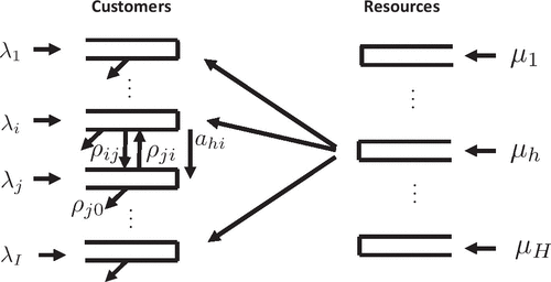
Notes. For and , λi and μh are the arrival rates for customers of class i and resources of type h, and ρij represents the class change rate from customer queue i to queue j. Finally, ahi is the probability of successful matching between type h resources and class i customers.
One motivation for the current setting stems from the organ transplant application, where both the class change and matching failure features have been observed and studied. Fluid models that capture patients’ health change were proposed in Akan et al. (2012) to study the organ allocation control problems over a finite time horizon. The optimal policy is of priority type, where the priority indices dynamically depend on the shadow price process of the optimal control problem. The stochastic version of this problem was investigated in Khademi and Liu (2021), where the asymptotic optimality of the dynamic priority rule is established under a strictly overloaded condition in fluid scaling. In another related work, motivated by patient health deterioration in hospitals, Hu et al. (2021) developed a multiclass many-server queueing system, where customers of class i can move to adjacent classes i − 1 and i + 1. Focusing on the fluid dynamics of the setting with two customer classes, they developed a modified rule to optimize a long-run average cost function and investigated the stability of the state process under the proposed policy. They further studied an associated transient control problem (see Section 2 for a more complete literature review of related works). Considering a general multiclass bipartite matching system in a Markovian setting, our current work exploits the class change feature to develop a stability condition under which the system is stable for any arrival rates of customers and resources and any admissible control, and propose asymptotically optimal policies by studying a simple linear program (LP).
We consider a decision maker (DM) who is interested in maximizing the long-run average expected matching values and minimizing the long-run average expected cost. To this end, a bicriteria objective is formulated as a single objective via a linear combination of the two objectives with flexible weights. By this transformation, we study the bicriteria objective as a minimization problem, where the bicriteria objective is referred to as the weighted cost function. Both the class change and matching failure play important roles in designing efficient control policies. To showcase the complexity, we consider a simple system with two customer classes and one resource type. Customer class 1 has high matching value and low cost, whereas customer class 2 has low matching value and high cost. This assumption is motivated from a healthcare application, where class 1 customers correspond to patients in better conditions comparing with class 2 customers in more urgent conditions. The matching value may represent the treatment effect and the cost may include the waiting and abandonment costs. We observe that without the class change or matching failure features, if the objective is to maximize matching values, customer class 1 should be prioritized, whereas if the objective is to minimize the cost, a rule developed in Atar et al. (2010) should be applied (noting that the service rates for both classes are the same in this setting and equal to the arrival rate of the resource). Clearly, designing an efficient policy for our bicriteria objective depends on the weighted cost and should properly balance the matching values and costs. Now, if we include the customer class change feature, the outflow from each queue before matching consists of the abandonment and transitions to other queues, and similarly the inflow into each queue includes the transitions from other queues in addition to the external arrivals. When considering minimizing the cost, a modified rule was developed in Hu et al. (2021) for which the class change rates appear in the indices of the rule. As shown in our Section 4.2, these modified indices can be characterized in terms of the inverse of a matrix that collects the class change and abandonment rates, see the matrix P defined in (12). Finally, the introduction of matching failure will reduce the priority of the corresponding queue. The larger the matching failure probability, the less chance we allocate the resource to this queue. For a general multiclass bipartite system with multitype resources, the interplay of different features becomes more complex. Our work provides a unified approach to develop efficient policies in the presence of all these features.
1.2. Main Contributions and Results
Our main contributions and results are summarized as follows.
We provide a suitable stability condition (Assumption 1) on the class change and abandonment rates, under which the matching system is stable for any arrival rates of customers and resources and under any admissible control. The stability condition does not require all the abandonment rates to be positive. Instead, it exploits the class change structure and requires the existence of a class transition path from the customer queue without abandonment to a queue with abandonment. This condition can be applied for general parallel queues with class change.
We create a deterministic fluid control problem (FCP) that serves as a lower bound for the original queueing control problem (QCP) under any admissible control as the planning horizon T approaches infinity (Proposition 1). We introduce a class transition rate matrix P (see (12)) that can capture the class change and abandonment feature, show that P satisfies some regularity conditions (see Section 4.2.1 for details) under the established stability condition and characterize important properties of (Lemma 1). These results on P play a crucial role in establishing the lower bound in Proposition 1. Moreover, using , the FCP can be reformulated as a simpler LP that can be solved efficiently.
We solve the FCP analytically for two low dimensional matching systems with two classes of customers and two types of resources (known as X models), which may be of independent interest for applications, to illustrate how the class change and matching failure impact the optimal policy. The first system models a transplant queueing system with two patient classes (“Sick” and “Healthy”) and two organ types (“Low-quality” and “High-quality”). By Healthy, we mean a patient whose health condition is not severely deteriorated. We observe that the optimal policy is of assortative or priority type depending on a threshold, which is characterized in terms of the class change and abandonment rates, and the probability that Healthy patients decline Low-quality organs (Lemma 2). For the second matching system, we assume that there is no matching failure. The optimal policy is a simple index policy with indices given as the products of the linear cost (row) vector c and the columns of the matrix . The policy is thus referred to as the rule. It generalizes the well-known rule developed in Atar et al. (2010) and the modified rule developed in Hu et al. (2021) to an X matching model (Lemma 3).
We develop a large-scale asymptotic framework under which we propose a randomized matching policy for the QCP based on the optimal solution of the FCP and show that the proposed policy is asymptotically optimal under both the long-run average cost criterion and the ergodic cost criterion. Under the asymptotic framework, the volumes of both demand and supply are assumed to be high and of order (the factor n measures the size of the system, e.g., the total demand rate). We show that for sufficiently long planning horizon T, the FCP lower bound is attained under the proposed policy as the system size , and furthermore, for sufficiently large system with size n, the same FCP lower bound is attained under the proposed policy as the planning horizon (Theorem 1). The former result is the asymptotic optimality under the long-run average cost criterion and the latter gives the asymptotic optimality for the ergodic cost. These two results yield the interchange limit theorem for the state process and the matching process as T and n both approach infinity (Theorem 2). An important tool to prove these results is a Lyapunov function (see (44) and (50)) that is constructed using the M-matrix property of the class change rate matrix P. In particular, we show that the fluid limit (derived as ) of the state process under the proposed policy is a reflected ordinary differential equation (ODE) that is also known as a projected dynamical system. Using the associated variational problem and constructing a Lyapunov function, we show that the reflected ODE admits a unique equilibrium point that is exponentially stable (Proposition 5). Next, with a similar Lyapunov function, we make evident that the matching system under the proposed policy is ergodic (derived as ) and the fluid limit of the stationary distribution turns out to be the unique equilibrium point of the reflected ODE (Proposition 7). We believe that the constructed Lyapunov function can be potentially used to analyze the stability of parallel queues with class change under different types of policies.
1.3. Organization of the Paper
The rest of the paper is organized as follows. Section 2 reviews some related literature on matching queues, queues with class change, and scheduling control of multiclass queues. In Section 3, we develop the queueing model and the QCP. In Section 4, we formally introduce the FCP and the stability condition under which the FCP is reformulated as a simple LP, and prove that the FCP provides a lower bound for the QCP under any admissible control policy. In Section 4.4, we propose the randomized matching policy based on an optimal solution of the FCP. Section 5 studies two X matching systems and solves the corresponding FCPs to provide insights on how the class change and matching failure impact the optimal policies. Section 6 is devoted to constructing the asymptotic large-scale framework. In Section 6.1, we show that the proposed policy is asymptotically optimal under both the long-run average cost and the ergodic cost criteria. The detailed asymptotic analysis is provided in Sections 6.2 and 6.3. Section 7 conducts some numerical experiments using simulation. Section 8 discusses some of the assumptions that we make in the model and their implications and potential relaxations. All the proofs are presented in the appendix.
2. Literature Review
There are several streams of literature related to our study.
2.1. Allocation Control in Bipartite Matching Systems
The bipartite matching models have been widely used in organ transplant applications. For example, Hasankhani and Khademi (2021) extended the fluid model of Akan et al. (2012) to incorporate fairness constraints and showed that the optimal policy is still of a dynamic priority rule type. Ata et al. (2021) advanced the fluid transplant model to incorporate patient choice in accepting/declining the offered organ and showed that under some natural assumptions there exists a unique Nash equilibrium. The current literature on organ transplant applications mainly uses deterministic fluid models to address a variety of decision-making problems. In the current work, we consider a stochastic bipartite matching system and develop asymptotically optimal policies construced by the corresponding fluid model. The fluid model was also considered in Arnosti and Shi (2020) for the public housing application. They studied a matching queue with strategic waiting agents, where the DM has to strike a balance between targeting individuals with the highest need (fairness) and matching individuals with the resources that produce high value (efficiency). The recent work by Ding et al. (2021) studied a matching queue where the DM allocates the resource to the customer with the highest score, which is the sum of customer’s waiting time and matching score. The system is formulated as a stochastic model, the authors studied a fluid sample path of the system and developed an efficient algorithm to analyze the steady state of the fluid sample path. In the study of a ridesharing system, Özkan and Ward (2020) studied a stochastic matching system of drivers and customers with time-varying arrival rates. They developed asymptotically optimal matching policies based on a continuous linear program for a finite horizon control problem. Compared with this work, we consider a Markovian system which allows class change for a long-run average control problem and prove the asymptotic optimality under both long-run average and ergodic cost criteria.
All the aforementioned works including the current work focus on optimizing the demand side of the system and the supply is either matched or wasted, and thus can be viewed as one-sided controlled matching systems. If resources can also be queued in addition to customers, the system becomes a two-sided controlled system. For example, Aveklouris et al. (2021) proposed a two-sided matching queue with generally distributed patience times and studied the tradeoff between making quick valuable matches and waiting to make better decisions with the risk of losing impatient demand and supply. Afeche et al. (2021) studied the design of matching topology in a multiclass multiserver queueing system under a first come first served - assign longest idle server (FCFS-ALIS) service discipline. Beyond bipartite matching queues, Gurvich and Ward (2015) modeled a matching queue in which items arrive to their dedicated queue and wait to be matched with items of other queues based on match feasibility to minimize a finite-horizon cumulative holding cost function.
2.2. Queueing Systems with Class Change Feature
In addition to the aforementioned transplant queueing models and the work by Hu et al. (2021), Down and Lewis (2010) studied the effect of class change on the stability and optimal policies for a Markovian N model with two customer classes and two service stations (with multiple servers), where station 1 is flexible in serving both customer classes and station 2 is dedicated to customer class 2, and class 1 customers are allowed to be upgraded to class 2. In Cao and Xie (2016), a two-class single-server queue was studied, where class 1 customers can change to class 2. The queueing control problem is formulated as a continuous-time Markov decision process and the main results establish the existence of optimal nonidling stationary policies and the conditions under which a modified rule remains optimal. Xie et al. (2017) computed the stationary distribution of a two-class single-server priority queue that allows priority upgrade for nonpriority customers. These three works focus on the low-dimensional systems and do not consider abandonment or large-scale asymptotic setting. In Pang and Yao (2013), a collection of Markovian many-server queues, each queue with its own service pool, were considered, where a job waiting in a queue can switch over to another queue or abandon the system after an exponentially distributed time. The work is concerned with system performance analysis and establishes the fluid and diffusion limits under different large-scale regimes (quality-and-efficiency-driven and efficiency-driven regimes).
2.3. Scheduling Control of Multiclass Queueing Systems in Heavy Traffic
There is a significant literature on scheduling control of queues, where there is a fixed number of service stations/server pools in the system that serve randomly arriving heterogeneous customers. We review some related works in the many-server setting, focusing on the long-run average type objectives, or related to the X model. None of these works consider the class change feature studied in the current work. The works by Atar et al. (2010, 2011) developed the well-known rule for the Markovian multiclass many-server (in a single pool) queueing system with abandonments to minimize the long-run average cost, and showed that rule is asymptotically optimal under both the long-run average cost and ergodic cost criteria in the fluid scaling. For an overloaded (i.e., in the efficiency driven regime) multiclass many-server queue with multiple server pools, Stolyar and Tezcan (2011) proposed the shadow routing algorithm for reward maximization (SHADOW-RM) policy, and proved its asymptotic optimality for maximizing the long-run reward rate. For other works in scheduling overloaded multiclass many-server (in a single pool) queues, we refer the readers to the tutorial paper (Puha and Ward 2019) and the references therein. The literature on the ergodic control of many-server queues seems scarce. Armony and Ward (2010) designed a threshold policy for a single-class multipool many-server queue (known as the inverted V model) and showed that it is asymptotically optimal for minimizing the steady-state customer waiting time subject to a “fairness” constraint on the workload division in quality-and-efficiency driven regime. The ergodic control problem of the Markovian multiclass many-server (in a single pool) queues was studied in Arapostathis et al. (2015), and the study was extended to multipool setting in Arapostathis and Pang (2016). Both works are considered in the quality-and-efficiency driven regime. Comparing with these studies, our system assumes heterogeneity on both sides and class change feature for the customer side. We do not assume specific regimes and prove that the proposed policy is asymptotically optimal under both the long-run average cost and ergodic cost criteria.
As the simplest multiclass multipool queueing system, the X model has been studied in a series of work by Perry and Whitt (2009, 2011, 2013, 2015). Perry and Whitt (2009) studied two service systems (modeled as single-class single-pool many-server queues with abandonment) that can help each other when one encounters overload, and proposes an efficient fixed-queue-ratio-with-thresholds (FQR-T) control. In the sequels, Perry and Whitt (2011, 2013, 2015) developed fluid approximations and new algorithms for the overloaded X model under the FQR-T control. Our study of the X matching models focuses on exploring the impact of the class change rates and acceptance probabilities on fluid control problems.
3. Model Formulation
We study a bipartite matching queue where customers arrive to one side of the system and resources arrive to the other side. Customers and resources are differentiated by their classes and types. The customer class is indexed by so that there are totally I different customer classes. Customers of class i arrive to the system according to a Poisson process with rate λi and will join queue i on arrival. Customers in queue may abandon the system or join another queue while waiting. More precisely, the transition mechanism works as follows: Each customer in queue i is associated with I + 1 independent transition clocks, and for , the jth clock rings after an exponentially distributed time with rate ρij. If the jth clock rings first, the customer will join queue j, where queue j = 0 is interpreted as the outside of the system, that is, the customer will abandon the system. We assume that , which indicates that the customers in queue i will not leave their current position to join queue i again. There will be H types of resources, and the units of resource of type arrive to the system according to a Poisson process with rate μh. We assume each customer is matched with one resource unit and the matching is instantaneous, that is, each resource unit should be allocated to a customer immediately on arrival.
For each resource type h, let denote the index set of customer classes for which the resource type h is a feasible match. For each customer class i, let denote the set of resource types that are feasible for class i customers. Without loss of generality, we assume that for all h, and for all i, that is, for each resource type (respectively, customer class) there is at least one customer class (respectively, resource type) such that their matching is feasible because otherwise we can exclude that resource type (respectively, customer class) from analysis upfront without affecting the system. The matching topology is characterized by and for and and is assumed to be fixed.
On arrival of each resource unit, the DM will allocate it to the head-of-line of a feasible customer queue, and if all feasible customer queues are empty, the unit will be wasted and removed from the system. A match may fail and we let ahi denote the probability that a match of the customer class with the resource type is successful. If the match is successful, the customer leaves the system instantaneously with the offered resource unit; otherwise, the customer will stay in the system and the resource unit is wasted and removed from the system. Figure 1 provides a schematic view of the system. One application for a matching failure is that customers may have a preference over resource types and a customer who is offered a resource unit may decline it for a hope that the future offer is of the type that the customer has a higher preference for. For this application our approach assumes that customer decisions in accepting/declining the resource are exogenous; that is, we model those decisions by considering acceptance probabilities ahi. For example, for the application of the proposed matching system for transplant systems, all the simulation models for organ allocation purposes developed by the United Network for Organ Sharing (LSAM for liver, TSAM for lung and heart, and KPSAM for kidney and pancreas) consider the acceptance probabilities for patients based on past observations (UNOS 2021). Another example is in ride sharing applications, where a customer may decline the offered driver with a probability that may depend on different factors (Özkan and Ward 2020). Another application for a matching failure is that the matching process is disrupted. For example, in a communication channel, packages sent from a supply node to a demand node may get lost or corrupted.
We now mathematically formulate the problem. Let be a complete probability space. All the random variables and stochastic processes in this section are assumed to be defined on this space. The expectation under the probability measure will be denoted by . For , denote by the number of customers of class i in the system at time t, the number of successful matches of resource type h to customer class i up to time t, and the number of resource units of type h assigned to customer class i up to time t. Let and , respectively, represent the Poisson arrival processes of customers of class i and resource units of type h. Because the transition clocks associated with each customer are independent and exponentially distributed, the transition processes between customer queues can be formulated using independent Poisson processes. Let be independent unit rate Poisson processes, which are independent of the arrival processes . Then, the number of customers in queue i that join the customer queue j by time t can be formulated as Consequently, the state process can be described as follows: For and ,
Furthermore, the random variables are assumed to be independent of the arrival processes and the Poisson processes
The allocation policy is represented by a matrix-valued stochastic process : At time t, , where each equals zero or one and there is at most one element equal to one in each row, that is, for each and for . Suppose that a unit of type h resource arrives at time t. If for some , the unit is assigned to the customer queue i. Otherwise, if for all , the unit will be wasted. We study nonanticipative allocation policies. To this end, define the following filtration: For
Given an admissible control policy , the allocation process and the successful matching process can be formulated as follows. Let denote the arrival time of the kth unit of resource type h (that is, the kth arrival time of the Poisson process ). We have for ,
Note that can also be completely characterized by the jump times of .
An assigned unit may result in a successful match or a waste. Let be an independently identically distributed (i.i.d.) sequence of Bernoulli random variables with successful probability ahi, which represents the probability of a successful match between customer class i and resource type h. Thus, for ,
We assume that for each the vector is independent of and all the external arrival processes and for and (noting that denotes matrix transpose). That is, the success of a match only depends on the class and type of the pair and is independent of the aforementioned system information.
Next, we provide the elements of the objective function. The DM considers the following factors in the matching system: (1) the value of successful matches, (2) the waiting cost of customers, and (3) the abandonment cost of customers. (One can also consider the wastage cost of a resource, see Section 8.) Specifically, the DM seeks to maximize the average value of the successful matches and minimize the average waiting and abandonment costs over a finite planning horizon (to establish asymptotic optimality, we will eventually consider a long horizon by letting ). Let denote the value of a successful match between a customer in class i and a resource unit of type h. Let denote the linear holding cost that a class i customer imposes to the system per unit time, and denote the cost that is imposed to the system if a customer of class i abandons the system. Let denote the total expected cost of holding and abandonment per customer of class i per unit time. Given an admissible allocation policy , the expected average holding and abandonment cost over the time interval is given by
In addition, the expected average value of successful matches is given by
Because the DM seeks to choose admissible policies to minimize the objective function (5), and to maximize the objective function (6), we combine the two objectives into one and consider a weighted average of the two objective functions by assigning a weight of to the minimization objective (5) and to the maximization objective (6), where . Without loss of generality, we present the objective in the minimization sense; that is, we consider the following expected “weighted cost” of an admissible allocation policy :
The direct analysis of the control problem (8) is rather complex, and the standard numerical methods do not apply because of the curse of dimensionality. Our goal is to (i) develop a stability condition under which a simple LP, referred to as the fluid control problem (FCP), provides a lower bound for the queue control problem (QCP) (8) when , (ii) construct asymptotically optimal allocation policies for the QCP (8) in a suitable large-scale setting by using the optimal solution of the LP, and (iii) show that under the proposed policy, the matching system in the large-scale setting is ergodic with a unique stationary distribution. The next section develops the FCP of interest.
4. FCP
In this section, we construct the FCP by considering the expectation of the stochastic processes constructed previously. We develop a suitable stability condition (Assumption 1) under which the FCP attains a simple reformulation, and its optimal value provides a lower bound for the QCP (Proposition 1).
4.1. Construction of the FCP
We first establish a lemma that will be used in the construction of the FCP. Recall the allocation process and the successful matching process from (3) and (4). It can be shown that for all . Taking expectation in (1) yields that for and
Next, taking expectation in (2), we have
Now define and for . We introduce the following deterministic control problem associated with the state process and the control process . This control problem serves as a transitional step to introduce the FCP of interest.
Given and , the transitional control problem selects to minimize
We are interested in analyzing the system for a long time horizon. Letting enables us to establish a deterministic control problem in equilibrium, which will be the focused FCP. Roughly speaking, we will think of admitting an equilibrium point such that as , and then the long-run average will converge to as well when Instead of considering directly, we study the proportion and denote by its formal equilibrium, that is, as . In other words, represents the proportion of type h resource assigned to class i customers.
(
The relationship between the original QCP (8), the transitional control problem (10), and the FCP (11) is characterized in Proposition 1. Before stating the result, we present the following stability condition. Let and . The set (respectively, ) collects the indices of customer queues for which the abandonment rate is positive (respectively, zero).
(
Assumption 1 says there exists at least one customer queue with a positive abandonment rate, and for any customer queue without abandonment, there exists a transition path from this queue to a customer queue with abandonment through class changes.
4.2. FCP Reformulation
We study some structural properties embedded in the FCP that will be crucial in further analysis. To that end, considering the matrix form of (11b), we let , and introduce the following matrices:
Now, equations in (11b) can be represented as .
The matrix plays a crucial role in the analysis throughout the paper. In Section 4.2.1, we present some important structural properties of . Next, in Section 4.2.2, we propose a reformulation to the LP (11), which facilitates the interpretation of the optimal solution.
4.2.1. Structure of Matrix and Its Inverse.
We develop some important properties of in Lemma 1. A square matrix is called a nonsingular M-matrix if it can be expressed as , where is the identity matrix, B is a matrix with nonnegative entries, and the scalar s is greater than the spectral radius of B. Nonsingular M-matrices appear in many applications and have rich properties (see Plemmons (1977) for a collection of equivalent definitions for M-matrices.
Under Assumption 1, (i) is a nonsingular M-matrix, (ii) its inverse has positive diagonal entries and nonnegative off-diagonal entries, and (iii) for and , the (i, j)th entry of is positive.
The proof of Lemma 1 is provided in Appendix B.1, and the key is to observe that the matrix P is a weakly chained diagonally dominant matrix.
For convenience, let . The entries of the matrix A could be rather complicated. In Appendix A, we investigate a special case when P is upper triangular to shed some light on its structure.
4.2.2. FCP Reformulation Presentation.
In this section, we provide a reformulation to the FCP (11) that will pave the way to provide insights on its optimal solutions. From Lemma 1, we have that , that is, Equation (11b) can be written as , and its substitution in Equation (11c) results in the following Equation (14b). Therefore, Formulation (11) can now be reformulated as follows:
The optimization problem (14) is an LP with a bounded convex nonempty solution space and thus admits an optimal solution at the boundary.
Under Assumption 1, the FCP admits an optimal solution.
Denote by an optimal solution and the corresponding optimal state. One may interpret as the optimal proportion of type h resource assigned to customers of class i. For an optimal solution, if the ith constraint in (14b) becomes active, then ; otherwise, because . If the hth constraint in (14c) becomes active, all the resource units of type h are used; otherwise, the optimal solution wastes some of it. Furthermore, if the optimal solution constraints in (14b) are all inactive, that is, for all , the system is “strictly overloaded.” Consequently, the optimization problem (14) becomes a knapsack problem whose solution is a priority policy by sorting ’s. In this case, for resource type h, customers’ priority will be based on . The exact optimal solution of the LP depends on the matching topology (i.e., the index sets and for each i and h) and the system parameters . To provide insight on the structure of the optimal solution, we study two low-dimensional matching systems in Section 5.
4.3. Lower Bound on QCP
We now present Proposition 1 that shows that the FCP serves as a lower bound for the QCP as the time horizon tends to infinity. This enables us to construct asymptotic (in a sense that will be clear later in Section 6) optimal policies for the QCP by using the optimal solution of the FCP. First, we show the following Lemma 3 that says under Assumption 1 the matching system is stable under any admissible control, and will be used in the proof of Proposition 1.
Under Assumption 1, there exist positive constants C1 and C2 that are independent of t such that for any ,
Under any admissible policy π for the QCP (8) and for any ,
The complete proofs of Lemma 3 and Proposition 1 are provided in Appendix B.1. Roughly speaking, the first part of Proposition 1 is true because the constraints in the FCP are created from those of the original stochastic control problem, as well as having the same objective. The second part holds because by Lemma 3, , which makes the constraints in (10) converge to those in (11).
4.4. Proposed Policy for QCP
We construct a simple randomized allocation policy for QCP using an optimal solution of the FCP. Under Assumption 1, denote by an optimal solution and the corresponding state of the FCP with parameter . For each , let representing the probability of wasting a resource unit of type h. We consider a generalized Bernoulli random vector according to the probability distribution More precisely, we consider a random vector such that each component Zhi is Bernoulli distributed with success probability and . The distribution of Zh is then given by
Denote by the previously described allocation policy. Clearly, it is admissible. The policy is not work-conserving; a resource unit is wasted when it is assigned to a customer queue that is empty, no matter other customer queues that can accept the resource be empty or not. Nevertheless, in Section 6.1, we will show that this policy is asymptotically optimal when the system scale is large, and the resource units wasted in the previous situation are asymptotically negligible.
5. FCPs for Two X Models
We analytically solve the FCP for two X matching models and investigate how their solutions depend on the class change rates and the success probability of matching. In the first model, we study a transplant system with two patient classes and two organ types and establish an optimal policy that is of assortative or priority type depending on a threshold. The threshold parameter is given in terms of the class change and abandonment rates, and the success probability of matching (Proposition 2). For the second model, an X model with no matching failure is considered where the FCP only minimizes the linear cost. We show that a simple index policy, referred to as the rule, is optimal and generalizes the well-known rule developed in Atar et al. (2010) and the modified rule developed in Hu et al. (2021) to an X matching model (Proposition 3).
5.1. An X Model for a Transplant System
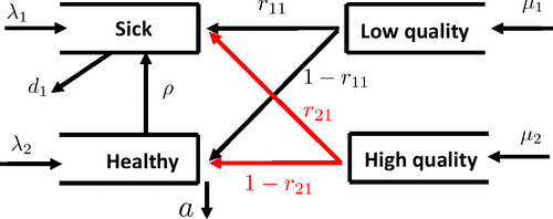
We consider a transplant queueing system with two patient classes (Sick and Healthy) and two organ types (Low-quality and High-quality). The arrival rates for Sick and Healthy patients are λ1 and λ2, and the arrival rates for Low-quality and High-quality organs are μ1 and μ2. Sick patients die with rate and Healthy patients become Sick with rate . We assume that Healthy patients do not die while waiting (i.e., ) and Sick patients do not become Healthy (i.e., ). We also assume that Sick patients accept both organs with probability one (i.e., ), Healthy patients accept High-quality organs with probability one (i.e., ), but accept Low-quality organs with probability . Figure 2 shows a schematic view of the system. In transplant queueing systems, it is natural to assume that , that is, the system is overloaded in the sense that the demand for organs exceeds the supply. Under this assumption, summing up (11b) over i = 1, 2 results in under any feasible allocation policy. Thus, no organ will be wasted (because of no available patients), which yields that the allocation rates must satisfy . The matrix and its inverse A are given by
In the FCP, the cost ci represents the pretransplant mortality, as well as the social costs corresponding to waiting on the list, and the matching values denote the posttransplant survival of a patient in class i on transplanting an organ of type h. It is natural to assume that and . That is, the posttransplant survival of Sick patients is less than or equal to that of Healthy patients. The FCP in (14) will be given by
Constraint (17b) is redundant because from the overloaded condition that , we have
Introduce
We note that , but C1 can be positive or negative or zero. For this system, we interpret the optimal allocation policy as being (i) assortative or (ii) of priority type. Assortative policies are those that assign high-quality organs to patients with lower risk (moderately healthy) and vice versa. We collect the optimal solutions of the FCP in the following Proposition 2; the proof is standard and provided in Appendix B.2.
When , we have is equal to one if , is equal to 0 if , and can take any value in if And is always equal to zero. When , the optimal solution is summarized in the following cases.
(1) If , and .
(2) If , and .
(3) If , and .
(4) If , any feasible point on the line is an optimal solution.
(5) If , and .
From Section 4.4, we can construct a randomized policy based on the solution of the FCP for QCP. For example, in Case (1), when , if , then This says proportion of High-quality organs should be assigned to Sick patients and proportion of High-quality organs should be assigned to Health patients. However, in view of the optimal solution and its associated optimal state, we can also interpret the policy being of priority type or assortative. In Case (1), indicating the type 1 (Low-quality) organs should prioritize class 1 (Sick) patients. Next, . This says if , all the type 2 (High-quality) organs are allocated to class 2 (Healthy) patients and , and if , the type 2 (High-quality) organs should prioritize the class 2 (Healthy) patients such that and the rest ( proportion) can be allocated to the class 1 (Sick) patients. In this way, we can propose an assortative policy for the QCP, which says the type 1 (Low-quality) organs should prioritize class 1 (Sick) patients and the type 2 (High-quality) organs should prioritize class 2 (Healthy) patients. Similar analysis can be applied to other cases. We summarize the results in Table 1.
However, not all optimal solutions of the FCP can be easily interpreted as being assortative or of priority type. For example, in Case (4) of the previous proposition, if we compute an optimal solution for which both and are within (0, 1) (this happens when the solution is in the interior of the line segment). In this situation, it is not straightforward to design an assortative or priority policies, and a randomized policy naturally arises, assigning proportion of Low-quality organs and proportion of High-quality organs to Sick patients, and the rest goes to Health patients.
The following two examples are concerned with two special cases to provide more insight: when and and when and .
|

Table 1. Intuition for Results in Proposition 2
| Case | Interpretation |
|---|---|
| (1) | The type 1 (Low-quality) organs should prioritize the class 1 (Sick) patients. |
| The type 2 (High-quality) organs should prioritize the class 2 (Healthy) patients, and any remaining organs will be allocated to the class 1 (Sick) patients. | |
| (3) | The type 2 (High-quality) organs should prioritize the class 2 (Healthy) patients, and if type 2 (High-quality) organs cannot satisfy all class 2 (Healthy) patients, the remaining requirements will be satisfied by type 1 (Low-quality) organs. |
| (5) | The type 1 (Low-quality) organs should prioritize the class 2 (Healthy) patients, and if type 1 (Low-quality) organs cannot satisfy all the class 2 (Healthy) patients, the remaining requirements will be satisfied by the type 2 (High-quality) organs. |
We consider the special case when and , in which the DM seeks to minimize pretransplant mortality, as well as social costs corresponding to waiting on the list. In terms of application, it means that the DM does not include posttransplant survival, that is, matching values, in the objective. This is aligned with practice for some organs. For example, UNOS allocation rules for liver and heart do not include donor risk profiles and in broad view are medical urgency based (OPTN 2021). We have
Thus, Case (5) of Proposition 2 does not happen. Proposition 2 provides the following insight into the optimal allocation: If the probability that class 2 (Healthy) patients accept type 1 (Low-quality) organs is less than the threshold , the optimal policy is assortative in that type 1 (Low-quality) organs are matched with class 1 (Sick) patients and type 2 (High-quality) organs are matched with class 2 (Healthy) patients. However, if the probability that class 2 (Healthy) patients accept type 1 (Low-quality) organs is greater than the threshold, the optimal policy prioritizes class 2 (Healthy) patients: High-quality and Low-quality organs will satisfy Healthy patients first, and the rest goes to the Sick patients.
We consider the special case when and , in which the DM maximizes the successful matching values, that is, posttransplant survival. We have
The threshold of the acceptance probability in (21) is given as , which only depends on the two matching values. From (22), we see that the relationship between and a is determined by the quantities and that represent the posttransplant survival difference between Healthy and Sick patients from the Low-quality and High-quality organs, respectively. More precisely, when , we have
If , then and ,
If , and , then and ,
If , and , then and ,
Thus, Case (5) of Proposition 2 happens only when and the acceptance probability a is large enough such that
Let be a lattice and be a function defined on it. The condition means that the function ϑ is supermodular (submodular). Becker (1973) showed that in a static matching market with equal-sized groups supermodularity (submodularity) of matching values results in a positive (negative) assortative matching, that is, mating of likes (unlikes). Results in Proposition 2 has an assortative flavor when . In particular, if , it seeks to maximize (the rate of assigning Low-quality organs to Sick patients) and minimize (the rate of assigning High-quality organs to Sick patients). Because of the existence of the acceptance probability a, the required condition becomes , with , which provides the following insight: Because the Healthy patients may decline Low-quality organs, the condition for positive assortative matching becomes “easier” to satisfy.
5.2. An X Model with No Matching Failure
In this section, we consider a matching system with two types of resources and two classes of customers. We assume that the matching process is perfect, that is, , and the matching topology is a complete bipartite graph, that is, and . The DM is interested in minimizing the linear cost by considering the LP (14) with and . Denote by the optimal value of the LP.
For this LP, if the system is underloaded or balanced, that is, , there is enough supply of resources for the demand of customers and the system will be empty under the optimal policy in the long run. When the system is overloaded, that is, , the optimal solution is a priority policy that assigns priority to each class according to the index for Recall that A is the inverse of the rate matrix P. We thus refer to this index policy as the rule, where c is understood to be the row vector (c1, c2) and the indices are given as the products of c and the columns of . The optimal solutions depend on the following two quantities:
Under the overloaded condition, U > 0 and , but it is possible that . Furthermore, the FCP is equivalent to the following LP:
Proposition 3 characterizes the optimal solutions of the LP in details. Its proof can be found in Appendix B.2, in which we also provide details on deriving the previous LP.
If , then with the optimal solution satisfying and
If , then , and the optimal solutions are given as follows.
(1) When (equivalently, ), and take their minimum feasible values, that is, Class 2 customers receive the higher priority from both types of resources.
If .
If such that .
(2) When (equivalently, ), and take their maximum feasible values, that is, Class 1 customers receive higher priority from both types of resources.
If .
If such that .
(3) When (equivalently, ), and can take any feasible values satisfying and , and the optimal value
We first understand the role of the quantities L and U in (i), and then in (ii) compare the cP−1 rule developed here with the cμ/θ rule.
(i) The quantities L and U are used to define the traffic intensities for the prioritized queues. In Proposition 3 part (1), from (23), we have
One can see that the ratio represents the traffic intensity for Class 2 customers when Class 2 is prioritized. Symmetrically, in Proposition 3 part (2), from (24),
Thus, the ratio represents the traffic intensity for Class 1 customers when Class 1 is prioritized. Under the corresponding priority policy, when the traffic intensity of the prioritized class is less than or equal to one, the prioritized class is always empty and the other class is always nonempty, otherwise, if the traffic intensity is greater than one, then both classes are nonempty.
Comparing with the well-known rule, the rule developed here only depends on the costs and class change rates, and does not depend on the resource arrival rates. In fact, different from the many-server queues considered in Atar et al. (2010, 2011) and Hu et al. (2021), in the bipartite matching queue with complete matching topology, there is no fixed “service rate” for each class of customers, instead each class of customers can be matched with all types of resources. In particular, in a many server queue there is a fixed pool of servers and each server serves class i customers with rate μi. However, in our bipartite matching queue, a “server” of type h arrives randomly over time and serves all customer classes with rate μh. Different resource types in our model impose different matching values, but in this example, matching values are ignored. (Recall that in an strictly overloaded system, for each resource type h, the priority is given by , which depends on matching values as well.) Furthermore, if there is only one resource type, the rule is reduced to be the modified rule as in Hu et al. (2021), and if there is no class change, the rule is simplified to be the rule, which shows that the index policy generalizes the rule and the modified rule to an X matching model.
6. Asymptotic Framework
This section develops an asymptotic framework, in which suitably scaled stochastic control problems attain the FCP lower bound as the system scale and the time horizon T grow to infinity. We introduce the parameter n that represents the system scale and can be considered as the average number of customers and resource units arriving during a unit time interval. We introduce a sequence of queueing systems as described in Section 3, indexed by . For the nth system, we append a superscript n to all system processes, random variables, and parameters. However, for simplicity, we assume that the Bernoulli random variables and its success probability ahi, and the matching value and cost ci in the objective function are all independent of n.
To construct the asymptotic setting, we study a large market setup in the following sense.
(
Furthermore, the matrix satisfies Assumption 1.
In the nth system, represents the number of customers of class i in the system at time t, is the number of successful matches of type h resource to class i customers up to time t, and is the number of resource units of type h assigned to customer class i up to time t.
(
We also recall that and respectively represent the Poisson arrival processes of customers of class i and resource units of type h for and and are independent unit rate Poisson processes, which are independent of the arrival processes . The state and control processes , and are described as follows: For , and ,
The control problem for the nth system is to choose an admissible allocation policy to minimize the following fluid scaled average cost function
The previous control problem, the same as the original control problem (8), is intractable in direct analysis. Our goal in this section is to show that the proposed randomized allocation policy associated with the fluid-limit parameter (see Section 4.4 for the definition of the policy) is asymptotically optimal in the following sense:
In (29) and (30), we consider both orders of the two limits as and . To establish (29), we first let to derive a deterministic fluid limit of under the proposed policy and then let to study the stability of the fluid limit, whereas in the study of (30), we first let to reach the steady state of (which is a Markov chain under the proposed policy) and then let to derive the fluid limit of the steady states. In particular, the study of (30) yields the ergodicity of the Markov chain under the proposed policy for each sufficiently large n. The allocation policies satisfying (29) and (30) are thus asymptotically optimal under the long-run average cost criterion as in (29) and the ergodic cost criterion as in (30).
6.1. Asymptotic Optimality of the Proposed Policy
Let and be an optimal solution and the corresponding optimal state of the FCP associated with Following Section 4.4, we construct the randomized policy based on . Thus, does not depend on n. We consider for each of the nth system. We next present our main results: Theorems 1 and 2. The proofs will be decomposed into various intermediate results shown in Sections 6.2 and 6.3. The complete proofs of both theorems are provided in Appendix B.3.3.
The first result is on the asymptotic optimality of the proposed policy.
The proposed policy is asymptotically optimal under the long-run average cost criterion as in (29) and the ergodic cost criterion as in (30).
The next theorem establishes the interchange limit theorem for the bipartite matching system under the proposed allocation policy .
Under the proposed policy is a Markov chain for each n, and if there exists such that when , it is irreducible, then for
Furthermore, for and ,
Although the proposed policy is independent of n, it is constructed by the fluid-limit parameter . In practice, one needs to identify n and the model parameters to compute , for example, However, the system scale n may not be easily identified. Instead of considering the fluid-limit parameters , one can construct the proposed policy according to an optimal solution of the FCP associated with the unscaled system parameters. To be more precise, assume that we have the Nth system with N being large but unknown. Under Assumption 2, the FCP associated with can also be reformulated as a simple linear program and admits an optimal solution with the optimal value . Now one can show that sufficient conditions in Wets 1985 (proposition 8) hold and by Wets 1985 (theorem 2), the linear program FCP associated with is continuous in its parameters. It follows that , which yields
Denote by the proposed policy according to . Combining (29) and (30) with (31), when T is also large, we have
As mentioned in Section 4.4, the randomized policy we propose is not work-conserving. In Corollary 1, we show that the policy is asymptotically work-conserving. For the kth arrival of the type h resource, let denote the generalized Bernoulli random according to the probability distribution (see Section 4.4 for more explanation on the distribution). Then the process of successful matching can be formulated as
Recall that is the sequence of arrival times of the Poisson arrival process of type h resource. Now define for ,
The quantity represents the number of type h resource units assigned to customer queue i over the time interval assuming the queue is nonempty for each assignment. The difference gives the number of type h resource units that are assigned to customer queue i and are wasted because of the emptiness of the queue over the time interval . The following result as a corollary of Theorem 2 shows that the long run average wasted resource is asymptotically negligible in the fluid scaling. The proof can be found in Appendix B.3.3. In Section 7, we numerically explore the convergence behavior of with respect to n and t (see Section 7 for the related discussion).
We have the following interchange limit result for .
The rest of the section will focus on the proofs of the two main theorems. Section 6.2 focuses on the study of (29). We first derive a deterministic limit, known as the fluid limit, of as under the proposed policy, and then study the stability property of the fluid limit as . In Section 6.3, we show that under the proposed policy, is a Markov chain admitting a stationary distribution and derive the fluid limit of the stationary distribution as In the following sections, we use the L2 norm for
6.2. Fluid Limit and Its Stability
We are interested in the asymptotic behavior of the matching system under the proposed policy as To that end, for a given T, we show that the scaled process under the proposed policy converges to a solution, denoted by , of a reflected ODE uniformly on . Then, the first natural question is: Does this dynamical system has a unique solution? Is , which is the corresponding optimal state of the FCP, an equilibrium point of ? The second natural question is: If converges to as , how fast is the convergence? This is equivalent to study the stability property of The main challenge in addressing these questions is that the dynamical system has a reflection boundary, which creates a type of discontinuity. We provide affirmative answers to these questions by constructing an appropriate Lyapunov function, adopting results in the generalized linear Skorokhod problem and the associated variational inequality problem for an equivalent projected dynamical system. The complete proofs of all results in this section are provided in Appendix B.3.1.
In the first step, we present a law of large number result for the successful matching process under the proposed policy. Recall from (33) that
By constructing proper martingales and applying convergence theorems for martingales, we can show the following Lemma 4.
Under the proposed policy , for any and ,
The following proposition establishes the fluid limits of the state and control processes under the proposed allocation policy
Under the proposed policy , for any T > 0 and ,
The proof of Proposition 4 follows a standard weak convergence argument. We first observe that is C-tight and uniformly integrable, and then show that its weak limit satisfies (38) and the generalized linear SP (39).
The next step involves exploring the stability properties of the reflected ODE given in (39). To ease notation, let function be such that for ,
Noting that is the corresponding state of the FCP under the optimal solution , the pair satisfies Constraint (11b), that is, Consequently, is an equilibrium point of the reflected ODE . The following proposition establishes the uniqueness of the equilibrium point as well as its stability.
The point is the unique equilibrium point of the reflected ODE , and it is globally exponentially stable; that is, there exist constants B > 0 and such that
Furthermore,
We provide here the main proof ideas of Proposition 5.
(i) The proof of the uniqueness of the equilibrium point in Proposition 5 relies on the observation that the reflected ODE is equivalent to the projected dynamical system (PDS) associated with and F, and the equilibrium points of the reflected ODE coincide with the solutions of the variational inequality (VI) problem associated with and F (Dupuis and Nagurney 1993, Nagurney and Zhang 2012). The rigorous definitions of the PDS and VI problem can be found in the proof of Proposition 5 in Appendix B.3.1.
(ii) A key tool for the proof of the globally exponential stability in Proposition 5 is an appropriate Lyapunov function. For the nonsingular M-matrix , there exists a positive diagonal matrix D such that is positive definite (Plemmons 1977). The Lyapunov function is defined as
(44)which measures a weighted distance from the point x to the equilibrium point
The following corollary follows from Propositions 4 and 5.
Under the proposed policy , for ,
6.3. Steady-State Analysis and Its Fluid Limit
Under the proposed allocation policy , the state process in the nth system is a Markov chain with the following generator , where is the set of measurable functions from to . For and ,
It is not clear upfront whether the Markov chain is irreducible because the transition rates can be zero among some customer queues. Nevertheless, we can consider the limiting behavior of the chain.
Under the proposed policy , for ,
When the chain is irreducible, it can be shown to be ergodic with a unique stationary distribution.
Under the proposed policy , there exists an such that when , if the Markov chain is irreducible, it is ergodic with a unique stationary distribution.
The proofs of the previous two propositions rely on constructing a similar Lyapunov function (see Appendix B.3.2 for the complete proofs). We consider the Lyapunov function defined in (44) and modify it for in the nth system. Define the matrix in the same way as in (12) with ρ replaced by ρn and r replaced by . Under Assumption 2, for large enough n, the matrix satisfies Assumption 1 and Lemma 1 still holds for . Then, there exists a positive diagonal matrix Dn such that is positive definite. Define the following Lyapunov function for any given ,
A crucial step is to study , which represents the rate of change of the weighted distance from x (a value of ) to and show that it decreases linearly in (see Lemma B.1 in the Appendix B.3.2).
7. Numerical Experiments
In this section, we provide numerical evidence for our results. We simulate a stochastic matching system and observe the performance of our proposed policy. In particular, we consider a heart transplant system with I = 4 queues for patients and H = 2 organ types. This categorization is inspired by the fact that health is a major factor for pre- and posttransplant survival for heart transplant and UNOS used four categories of “1A” (class 1), “1B” (class 2), “2” (class 3), and “Inactive” (class 4) for patient health group, where 1A denotes the sickest, 1B is less severe than 1A, 2 is less severe than 1B, and Inactive patients are not suitable for transplant (OPTN 2021). For organ type, donor age is crucial for posttransplant survival, and we consider donors with age [18,50) as type 1 and [50, 80] as type 2.
At each time the following sequence of events takes place in the simulation. First, for each patient queue i, a random number from a Poisson distribution with parameter is generated and patients are added to the corresponding queue. For each organ type h, a random number from a Poisson distribution with parameter is generated as the number of arrived organs of type h. For each arrived organ with type h, based on the given policy we decide which patient queue it will be matched to. Let i be that patient queue class. If patient queue i is empty, the organ is discarded. Otherwise, we offer the organ to the patient in the head of the queue, which is consistent with UNOS practice. We generate a uniform random number in and compare it to ahi to decide whether the organ is accepted or not. On success, the patient leaves the system. If the patient declines the organ, it is discarded, and the patient stays in queue. Third, we decide on the death (abandonment) and class change for patients. To that end, for each patient in the system we roll an -dimensional die with probabilities corresponding to abandonment and class change, that is, ρij for all , the result of which determines what will happen to the patient: Staying in the queue, abandonment, or moving to another queue.
We use Hasankhani and Khademi (2017) to estimate the parameters of the model. We consider each period as a month. The initial number of patients in each queue is generated randomly according to a discrete uniform distribution between 200 and 250. The arrival rate of patient classes is approximately patients per month and that of organs is approximately organs per month. The death rate for patient classes is patients per month. The estimate of class change rates is shown in Table 2. To estimate the values for matching an organ to a patient, we use posttransplant life months. In particular, for type 1 organ, the posttransplant life months of four patient classes are estimated as , and for type 2 organ those are estimated as . For Inactive patients, we set posttransplant life months to be zero because they do not receive organs while in that state. For the holding costs in queue, we consider pretransplant costs while waiting on the wait list. Specifically, based on the results of Evans (1987) and adjustment for the inflation rate, we estimate a value of $319,010 per year for the holding cost for each patient class. However, to be consistent with match values, which are based on life months, we convert this yearly cost to life months. To that end, we note that in cost-effective analysis in healthcare, each life year is roughly worth $100,000 (Goodman 2016). Therefore, the holding cost for each patient class will be around 3.2 life months per month. To estimate the abandonment (death) costs, we use the expected life months gained due to transplantation, which are 194 months for class 1A, 187.7 months for class 1B, 114.5 months for class 2, and 0 months for Inactive patients. We assume that two objectives of minimizing cost and maximizing value have the same weight and set and . For this system, and and . The value of the lower bound, the optimal objective function, is .
|
Table 2. Estimates of Patient Class Change Rates
| 1A | 1B | 2 | Inactive | |
|---|---|---|---|---|
| 1A | — | 0.1344 | 0.0036 | 0.1344 |
| 1B | 0.56448 | — | 0.0156 | 0.07029 |
| 2 | 0.0036 | 0.0213 | — | 0.07479 |
| Inactive | 0.0063 | 0.0036 | 0.0093 | — |
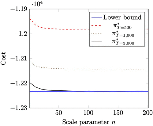
We explore the convergence behavior with respect to n and T. To that end, we set three values for T, that is, T = 500, T = 1,000, and T = 3,000 and then change n from 1 to 201 with increments of 10, that is, . We report the average numbers for 30 simulation replications. Figure 3 shows the value of the scaled cost and lower bound. The result for T = 500 is denoted by a dashed red curve, for T = 1,000 by a dotted brown curve, and for T = 3,000 by a solid black curve. As can be seen, the objective of the nth system stabilizes after n = 50 for all three cases for T. For T = 500, the scaled cost converges to −11,981, and for T = 1,000, it converges to −12,142. When T = 3,000, it converges to −12,231.5, which is roughly equal to the lower bound optimal value .
Note. The subscript in denotes that is applied when T = t.
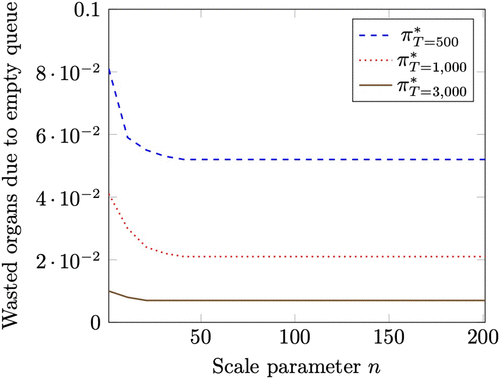
Furthermore, recall that the proposed policy will discard an organ upon its arrival if the result of the randomization is an empty queue. For example, in our numerical result, and if an organ of type 1 arrives and queue 3 is empty, it will be wasted. In this section, we numerically find in our simulation and present it in Figure 4, which by Corollary 1 is asymptotically negligible. In particular, Figure 4 shows that the average (over simulation runs) of the scaled number of organs wasted because the corresponding queue is empty on organ arrival. For T = 500, T = 1,000, and T = 3,000, the scaled wasted organs stabilize at 0.052, 0.021, and 0.007, respectively. The quantity roughly represents the number of organs that are discarded because of the emptiness of the assigned patient queues over the time interval . Also recall that the total arrival rate of the two types of organs is per month. Therefore, for T = 500, there are organs wasted during 500 months out of roughly 150 × 500 = 75,000 total organs. Such wastage is indeed asymptotically negligible.
In addition, we assume that if an organ is declined by a patient, it will be discarded. Next, we construct a policy that assigns organs to queues as does, but if the patient in the head of the queue declined the organ, the policy offers the organ to the next patient in that queue and continues this process until the organ is accepted by a patient or all the patients in the queue declined it. Our simulation results for T = 3,000 and n = 201, where the objective value is essentially equal to the lower bound, shows that the improvement of policy over is around 6%. This 6% improvement is notable because if a declined organ is eventually accepted, it will improve the objective function by increasing the life years instead of having a waiting cost. Under the policy , the acceptance probability for each organ becomes larger because it can be offered multiple times. See Section 8 for more discussion on the acceptance probabilities. In fact, does not fall into the set of admissible policies we define for the contact acceptance probability.
8. Discussion
In this section, we discuss some major assumptions in the model and the implications of their relaxation. First, we assume that resources will not queue; for example, in the transplant application, if an organ arrives and finds all queues empty, it will be wasted. This is a simplifying assumption, but it is not restrictive in overloaded systems, that is, when the demand significantly exceeds supply. We make this argument rigorous in the following way: The scaled overall allocation process for a resource converges to the arrival process of that resource type. To that end, the first step is to observe the following result.
If in (11), for all .
It implies that if customer queue i is positive in equilibrium, all the resources that supply patient queue i are exhausted. Let . We call the system “overloaded” if ; that is, there are enough positive queues in equilibrium such that all resource types are exhausted. Therefore, we have the following result.
If the system is overloaded in the sense mentioned previously, for each ,
The proofs of both results can be found in Appendix B.4. Second, we assume that if a resource is declined by a customer, it will be wasted. In organ transplant systems, however, if a patient declines an offered organ, it will be offered to the next patient in the waiting list based on patient scores. However, formulating the general allocation policy is challenging. In fact, if the patient in the head of the queue declines the organ, the policy should check whether there are other patients in that queue. If there are, it should check whether this patient accepts the organ or not by considering another Bernoulli random variable. This process continues until there are no more tried patients or the number of feasible offers are exhausted. If the process has to continue and all patients of the current queue have been tried, the policy must decide what queue is next. Therefore, the policy must completely characterize the path for organ offer, which makes the analysis challenging. Current fluid models in the literature approximate this process by considering the overall probability of organ acceptance. Specifically, let N denote the maximum number of times an organ can be offered. Recall that ahi is the probability that a class i patient accepts an organ type h. Thus, assuming queue i has at least N patients, the probability of eventual organ acceptance is , which is used instead of ahi in Equation (11b) (Akan et al. 2012). Nonetheless, our proposed model applies to organs with short cold ischemic time. For example, unlike a kidney with a cold ischemic time of 48 hours, a heart only has a cold ischemic time of 4 hours, making it difficult to reoffer it after a decline. In our numerical results, we consider a policy that assigns organs to patient classes as , but when the head of the queue patient declines the offered organ, it will offer it to the next patient in line until the organ is accepted or the organ is offered to all patients in the queue and declined. The probability of organ acceptance becomes and is state dependent. Our results show that the improvement in the objective function of over is around 6% for large n and T.
Third, in the model, we assume that there is no cost for resource wastage. The total wastage for resource type h up to time t is . If the wastage cost of one unit of resource type h is , the average wastage cost will be . This addition will only add a corresponding term in the objective function and the constraints will not change. Because we have already showed the asymptotic results for , all the results will hold by adding this extra term.
Finally, our proposed policy is randomized, and on arrival of a resource, a queue is determined randomly for assignment. If the queue is nonempty, the resource is assigned to the head of the queue; otherwise, the resource is wasted. In Corollary 1, we show that this randomized policy is asymptotically work-conserving. In our numerical example in Section 7, we show that the impact of nonconserving property becomes negligible for large n and T.
9. Conclusion and Future Work
We studied a bipartite matching system where customers of different classes and resources of different types arrive and need to be matched. Customers will join a corresponding queue on arrival and may change their queue or abandon the system probabilistically. Resources on arrival will be matched to customers where a match may be unsuccessful. Resources will be wasted if the match is unsuccessful or no customer is in queues. The DM will incur a cost due to customer waiting and abandonment and will accrue a reward for successful matches. We constructed a corresponding fluid control problem, which is an LP, and proposed a randomized policy based on its solution for the original problem. We showed that under the fluid scaling the proposed policy is asymptotically optimal and interchange of steady state and fluid limit holds. We also investigated the structure of the proposed policy under two X models.
There are some natural paths for future work. First, we assumed that resources must be assigned on arrival and cannot be kept in inventory. Although this assumption may be appropriate for overloaded queues (Corollary 3) like transplant systems, in underloaded queues, these resources may be kept in queues to model matching systems more realistically. Second, a match will be successful in the model based on a probability distribution. However, customers may be strategic in deciding to accept or decline a resource by solving an optimal stopping problem. The equilibrium analysis of this extension will provide more insight about this feature of the problem. Third, we assumed that the parameters of the model are known. However, some of the model parameters may be unknown but can be learned over time by sampling. The analysis of regret for such matching systems can be an interesting topic for future investigation. Last, we used a fluid-based approach to analyze the model, but considering a diffusion-based analysis will provide further realism.
Appendix A. Additional Results
A.1. Structure of
We investigate a special case when P is upper triangular to shed light on the structure of . We consider an upper triangular (the lower triangular case can be treated similarly). The motivation for such an upper triangular matrix stems in healthcare queueing systems, where healthier patients become sicker over time while waiting for service. This can be done without loss of generality by ordering queue classes such that queue 1 (respectively, I) presents the sickest (respectively, healthiest) patient group. For this class of problems, we provide a closed form for and interpret the results. Introducing , we have
The matrix is given as follows:
For i < j, the previous formula enumerates all the paths from queue j to queue i and adds the ratio of the product of class change rates in the numerator to the product of total out-class rates in the denominator. For example, for i = 1 and j = 4,
Appendix B. Proofs
We collect all the proofs in this appendix.
B.1. Proofs for Section 4
We start with some definitions on matrices. For an I × I square matrix C, its ith column is called weakly diagonally dominant (WDD) if and is called strongly diagonally dominant (SDD) if . The matrix C is called column WDD (respectively, SDD) if all its columns are WDD (respectively, SDD). The direct graph of matrix C consists of the vertex set with an edge from i to j if the (i, j)th entry is nonzero. A matrix is called weakly chained diagonally dominant (WCDD) if (i) it is column WDD and (ii) if a column i is not SDD. There exists a path in the direct graph of the matrix from vertex i to a vertex whose associated column is SDD. Observe that under Assumption 1, the matrix defined in (12) is WCDD. From Bramble and Hubbard (1964), the matrix is a nonsingular WDD M-matrix. From Plemmons (1977), exists and A has nonnegative entries. Finally, being an M-matrix, for some nonnegative matrix B and a positive constant s that is greater than the spectral radius of B. It follows that , which implies that the diagonal entries of A must be positive. Finally, we show that for and , if there exist such that , then Fix such a pair of i and j. We consider the linear equation , which yields and Because A has positive diagonal entries and nonnegative off-diagonal entries, and Suppose . We claim that all for and yj = 0, which is a contradiction to . Thus we must have . Under the assumption that , we consider the ith component of and have
Under Assumption 1, the FCP formulation is equivalent to the LP (14). The LP formulation (14) is nonempty because if we set all , all three set of constraints are satisfied. Also, the solution space of (14) is bounded; in the first set of constraints, all coefficients on the left-hand side are nonnegative and the right-hand side is also nonnegative with an inequality sign of . The second and third set of constraints clearly create a bounded region. Furthermore, all constraints are hyperplanes, so the solution space is convex. The result simply follows from the fundamental result in linear programming. □
Recall and for . To show (16), for each and , define
We claim that for all and (it will be proved at the end). By summing s over all and taking , we have
Using the Gronwall’s inequality, we have for ,
Next,
Now from Lemma 1, for , there exists a such that . Using (B.3), we have
Let Then from (B.4), we have
Using Gronwall’s inequality again gives
Combining (B.2) and (B.6) gives
At last, we show that for each and . Let . We have
We note that for all . Let . Without loss of generality, we assume the i0th component decreases below zero at t0, that is, and for for some We also assume that neither of the other components are below zero over the interval If more than one component falls below zero at t0, we can consider the sum of these components. Now for , we have
The original stochastic control problem (8) and the transitional control problem (10) share the same objective function. Furthermore, the constraints in the transitional control problem (10) are created from those of (8), which shows that the set of feasible solutions for (10) is a relaxation of (8). This shows (15).
From Lemma 3, we have for
Now dividing (10b) by t gives for each
From (B.7), for any , there exists such that when Fix such a T0 and define
We note that is an admissible solution to the FCP (11) associated with system parameters , and is the corresponding state process. Letting denote the corresponding optimal value, then
Finally, by the continuity of the solution of the FCP with respect to its parameters (Wets 1985, theorem 2 and proposition 8),
Combining (B.8) and (B.9) yields
B.2. Proofs for Section 5
We consider two cases: (i) and (ii) .
In Case (i) the constraint (17c) is redundant. Therefore, the optimization is over the two-dimensional cube . We have because , and
In Case (ii), the second constraint (17c) is not redundant. When , Constraint (17c) is reduced to be , which always holds true. Consequently, Constraint (17c) is feasible. When and should take the maximum and minimum feasible values, respectively. That is
When should still take the minimum feasible value, while can take any feasible value. That is,
Now when , we need to compare the ratios with , where the latter is the slope of the boundary of Constraint (17c). When , the optimal solution is achieved when takes the minimum feasible value. That is,
Symmetrically, when , the optimal solution is achieved when takes the minimum feasible value. That is,
At last if , then any feasible point on is an optimal solution. This completes the proof. □
The FCP in (11) for this problem is given by
We have the matrices
To reformulate the previous LP, we consider
When , there exists solutions to the equation
Under such a solution, , which implies that the optimal solution of the FCP must be zero. Now suppose Adding the two state equations yields
Noting that one of ρ10 and ρ20 must be positive, we have . Therefore, for a nonidling scheduling control, there should be no waste of resources. Consequently, we have and at optimality. Using (B.10), we have
The nonnegativity of and can be written as
We next consider the objective function. We note that
Therefore, the reformulation of the FCP for this problem is given by
When , an optimal should take its minimum feasible value, when , an optimal should take its maximum feasible value, and when , an optimal can take any feasible value. Finally, using the explicit form of the matrix A, the index
(i) When and take their minimum feasible values, and Class 2 customers receives a higher priority from both types of resources. More precisely,
If , and ,
If L > 0, such that , and
When and take their maximum feasible values, and Class 1 customers receives a higher priority from both types of resources.
If , and
If such that , and
When , the value function equals zero and and can take any feasible values. □
B.3. Proofs for Section 6
B.3.1. Proofs for Section 6.2
From proposition 7.1 of Khademi and Liu (2021), the sequence of processes is C-tight and uniformly integrable (there is no matching failure in Khademi and Liu (2021), and the allocation process there is denoted by Un). From (4), and for , which implies that is also C-tight and uniformly integrable. Consequently, is C-tight and uniformly integrable. It suffices to show the convergence in probability.
We let and . We first recall from (4) that
For the first step (B.12), fix h and i, and for , define
We observe that and random variables and are independent of each other and of . Therefore,
Hence, is a martingale difference. Next define for ,
We show that is a martingale, that is, for s < t. To that end, observe that
Finally, we observe that
Observing that
Using Doob’s inequality, it follows that for any and as
This shows (B.12) and completes the first step.
For the second step (B.13), define for Noting that is a Poisson process, is an square integrable martingale, and its quadratic variation is given by
Now observe that
By Assumption 2, the second integral above converges to zero almost surely. For the previous first integral, we have
This shows (B.13) and completes the second step. This completes the proof. □
The sequence is C-tight and uniformly integrable. It suffices to show the convergence in probability. We first introduce the following scaled centered process. For ,
We note that and the latter is stochastically bounded. From the strong law of large numbers for Poisson processes together with Assumption 2 and Lemma 4, we see that in probability.
The fluid scaled state process can be represented by
Let
From Assumption 2, in probability, where
Next, is nondecreasing in t, and Hence, , where and are generalized linear Skorokhod mappings associated with and the identity reflection matrix presented in the appendix of Reed and Ward (2004). By the Lipschitz continuity of maps and , we have in probability, where
Finally, using the convergence of , we have
B.3.2. Proofs for Section 6.3
We first introduce the (projected dynamical system) PDS and (variational inequality) VI problem associated with and the function F defined in (40). Recall that ei denotes the I-dimensional unit vector with one being the ith component and zero for the other components. For , let , and define the set of inward normals at x by
When , we define
For an and , define as the projection of v at x along inward normals such that (i) if , and (ii) if ,
From chapter 1 of Nagurney and Zhang (2012), for any initial condition , the function is a solution to the PDS associated with and F if is absolutely continuous and for almost every t. The VI problem associated with and F is to find such that
Lemma 1 and theorem 2 of Dupuis and Nagurney (1993) yield that the pair solves the reflected ODE (39) if and only if solves the PDS associated with and F, and the equilibrium points of the reflected ODE coincide with the solutions of the VI problem.
To show the uniqueness of the , we note that a point can be an equilibrium point of the reflected ODE if either (i) or (ii) , such that for and . The unique solution for (i) is . Let’s now consider (ii). We note that results in
We next show the stability of . Recall the Lyapunov function defined in (44). Clearly, , V (x) > 0 for any , and as . Furthermore, we have that
From lemma 2.1 in Nagurney and Zhang (2012),
Considering the last equation (B.20), we see that
For the second term in (B.20), if , then β = 0 and the second term equals zero. Now if , then and . We further note that
Because is positive definite, letting κ to be a positive constant that is smaller than the eigenvalues and diagonal entries of , then is also positive definite. Consequently, we have
The results follows from the Lyapunov criterion for globally exponential stability.
Last, from (41), we observe that
From (42), , which yields that
We first establish Lemmas B.1 and B.2, which play an important role in the proof of (48) in Proposition 6. Recall the Lyapunov function Vn defined in (50).
There exists an such that when
From Assumption 2, there exists such that when , the matrix Pn is a nonsingular M-matrix. We let . For notational convenience, we let represent the total supply allocation rate to customers of Class i, and . From (47),
The quantity in (B.24) can be bounded by for some independent of n and x. In (B.25), the quantity satisfies
Hence, for , independent of x, converging to zero,
Also noting that for all and , where , independent of x, converges to zero as , now (B.25) can be rewritten as
We note that from Tartar (1971), the matrices Dn and D can be constructed such that as Then for any ,
Combining the estimate for (B.24), and (B.27) and (B.28), we have for some independent of n and x,
The result follows by taking . □
The next result shows that for a fixed time t, the expected value of the norm of the state process grows at most linearly in n for sufficiently large n.
There exists such that when ,
From the proof of Lemma 3, , where
Let and We then have
From Assumption 2, there exists such that
From (B.2), we have
Now from Lemma 1, for , there exists a such that . Noting that and , from Assumption 2, there exists such that
Then from (B.6), we have
Combining (B.30) and (B.31) gives
We now start the proof of Proposition 6. We first consider (48). Recall that is a Markov chain with generator . Also, . By assumption, has a finite second moment and is finite for any n and T. Therefore, the following process is a martingale for the defined quadratic
Thus, we have
Dividing (B.32) by n2, from Lemma B.1, we have
Let . Using Lemma B.2, we then have
By the comparison principle for solutions of differential inequalities . Finally, for some independent of n and t, we have
We now focus on proving (49). It suffices to show that
Following the proof of Lemma 4, we have that
Considering the first term in (B.38), we let for ,
Using the same proof as for in the proof of Lemma 4, we have for , as ,
Next using the strong law of large numbers for Poisson processes in t, we have for each almost surely. Finally, for any ,
The second term in (B.38) has the following quadratic variation:
(B.39) and (B.40) show that converges to zero in probability as and then . We next observe that , which is uniformly integrable for all t and n. Thus, (B.36) follows. To show (B.37), we consider the fluid scaled state process under the proposed policy . Let and . Then for and ,
Consider large enough n such that ρn satisfies Assumption 1. From the proof of Proposition 1, . From (48),
Now combining the previous convergence and (B.36) yields that
Consequently, (B.37) follows. □
We verify the sufficient condition of ergodicity in proposition 8.14 of Robert (2013). In particular, we consider the function for ( is the fluid scaled version of the Lyapunov function that is defined in (50)). We will show that for large enough n, there exists positive K and γ (possibly depending on n) such that
(a) If , then ,
(b) and ,
(c) The set is finite.
From Lemma B.1, for large enough n,
Let for ,
The right-hand side of (B.41) can be estimated as follows:
We next observe that from (B.42), when for some K large enough, Thus, we can choose K such that the quantity in (B.44) is less than
This shows condition (a). To show (b), from Lemma B.2, we have for each ,
Noting that for some , we have
B.3.3. Proofs for Section 6.1
We first prove (29). Let be an arbitrary limit along a subsequence of {n}. Using Fatou’s lemma, we have
Also, we have , and is an admissible control to the transitional control problem defined in Definition 1 with initial value and parameters . Thus, (B.45) is equivalent to
Finally, from Proposition 1, we have
We now consider the proposed randomized policy and prove the first part of (29). From Proposition 4, we have for each T > 0, and
Thus,
Corollary 2 yields that
We now prove (30). For any admissible control πn, from Proposition 1,
From Wets (1985), the LP (14) is continuous in its parameters; thus, we have
This completes the proof of the first part of (30). The theorem follows now. □
It is an immediate corollary from Corollary 2 and Propositions 6 and 7. □
For each , using the functional law of large numbers for i.i.d. sequence, we have
Using functional law of large numbers for the Poisson processes and the continuous mapping theorem,
The corollary follows now from Theorem 2. □
B.4. Proofs for Section 8
Recall that we have
We first observe that for because resource type h serves customer i, that is, and we know that Aii > 0 and ahi > 0. Therefore, for if , we can increase by a small enough and decrease the value of by still satisfying constraint. Thus, the value of and will decrease, which contradicts with the optimality of . □
Because processes and are only different in terms of the Bernoulli random variable for the success of each match, setting ahi = 1 in Theorem 2 yields for and ,
Because , we have
Strong law of large numbers for Poisson processes yields
Therefore, we have
References
- (2021) On the optimal design of a bipartite matching queueing system. Oper. Res. 70(1):363–401.Google Scholar
- (2012) A broader view of designing the liver allocation system. Oper. Res. 60(4):757–770.Link, Google Scholar
- (2016) Ergodic diffusion control of multiclass multi-pool networks in the halfin–whitt regime. Ann. Appl. Probabilities 26(5):3110–3153.Google Scholar
- (2015) Ergodic control of multi-class m/m/n + m queues in the halfin–whitt regime. Ann. Appl. Probabilities 25(6):3511–3570.Google Scholar
- (2010) Fair dynamic routing in large-scale heterogeneous-server systems. Oper. Res. 58(3):624–637.Link, Google Scholar
- (2020) Design of lotteries and wait-lists for affordable housing allocation. Management Sci. 66(6):2291–2307.Link, Google Scholar
- (2021) An achievable-region-based approach for kidney allocation policy design with endogenous patient choice. Manufacturing Service Oper. Management 23(1):36–54.Link, Google Scholar
- (2010) The cμ/θ rule for many-server queues with abandonment. Oper. Res. 58(5):1427–1439.Link, Google Scholar
- (2011) On the asymptotic optimality of the cμ/θ rule under ergodic cost. Queueing Systems 67(2):127–144.Google Scholar
- (2021) Matching impatient and heterogeneous demand and supply. Preprint, submitted February 4, https://arxiv.org/abs/2102.02710.Google Scholar
- (1967) Weighted sums of certain dependent random variables. Tohoku Math. J. 19(3):357–367.Google Scholar
- (1973) A theory of marriage: Part I. J. Political Econom. 81(4):813–846.Google Scholar
- (1964) On a finite difference analogue of an elliptic boundary problem which is neither diagonally dominant nor of non-negative type. J. Math. Phys. 43(1–4):117–132.Google Scholar
- (2016) Optimal control of a multiclass queueing system when customers can change types. Queueing Systems 82(3–4):285–313.Google Scholar
- (2020) OM Forum: Innovative online platforms: Research opportunities. Manufacturing Service Oper. Management 22(3):430–445.Link, Google Scholar
- (2021) A fluid model for one-sided bipartite matching queues with match-dependent rewards. Oper. Res. 69(4):1256–1281.Google Scholar
- (2010) The N-network model with upgrades. Probability Engrg. Inform. Sci. 24(2):171–200.Google Scholar
- (1993) Dynamical systems and variational inequalities. Ann. Oper. Res. 44(1):7–42.Google Scholar
- (1987) The economics of heart transplantation. Circulation 75(1):63–76.Google Scholar
- (2016) What is a year of life worth? Accessed November 1, 2022, https://www.forbes.com/sites/johngoodman/2014/12/22/what-is-a-year-of-life-worth/?sh=9491956ad982.Google Scholar
- (2015) On the dynamic control of matching queues. Stochastic Systems 4(2):479–523.Link, Google Scholar
- (2017) Efficient and fair heart allocation policies for transplantation. MDM Policy Practice 2(1):2381468317709475.Google Scholar
- (2021) Is it time to include post-transplant survival in heart transplantation allocation rules? Production Oper. Management. 30(8):2653–2671.Google Scholar
- (1963) Probability inequalities for sums of bounded random variables. J. Amer. Statist. Assoc. 58:13–30.Google Scholar
- (2021) Optimal scheduling of proactive service with customer deterioration and improvement. Management Sci. 68(4):2533–2578.Google Scholar
- (2021) Asymptotically optimal allocation policies for transplant queueing systems. SIAM J. Appl. Math. 81(3):1116–1140.Google Scholar
- (2012) Projected Dynamical Systems and Variational Inequalities with Applications, vol. 2 (Springer Science & Business Media, Boston).Google Scholar
OPTN (2021) OPTN policies. Accessed May 15, 2021, https://optn.transplant.hrsa.gov/media/1200/optn_policies.pdf.Google Scholar- (2020) Dynamic matching for real-time ride sharing. Stochastic Systems 10(1):29–70.Link, Google Scholar
- (2013) Heavy-traffic limits for a many-server queueing network with switchover. Adv. Appl. Probabilities 45(3):645–672.Google Scholar
- (2009) Responding to unexpected overloads in large-scale service systems. Management Sci. 55(8):1353–1367.Link, Google Scholar
- (2011) A fluid approximation for service systems responding to unexpected overloads. Oper. Res. 59(5):1159–1170.Link, Google Scholar
- (2013) A fluid limit for an overloaded x model via a stochastic averaging principle. Math. Oper. Res. 38(2):294–349.Link, Google Scholar
- (2015) Achieving rapid recovery in an overload control for large-scale service systems. INFORMS J. Comput. 27(3):491–506.Link, Google Scholar
- (1977) M-matrix characterizations. I. Nonsingular M-matrices. Linear Algebra Appl. 18(2):175–188.Google Scholar
- (2019)
Scheduling an overloaded multiclass many-server queue with impatient customers . Operations Research & Management Science in the Age of Analytics (INFORMS), 189–217.Link, Google Scholar - (2004) A diffusion approximation for a generalized jackson network with reneging. Proc. 42nd Annual Allerton Conf. Comm. Control Computing (University of Illinois, Monticello, IL), 983–995.Google Scholar
- (2013) Stochastic Networks and Queues, vol. 52 (Springer Science & Business Media, Boston).Google Scholar
- (1992)
Two-sided matching . Aumann R, Hart S, eds. Handbook of Game Theory with Economic Applications, vol. 1 (North Holland, Amsterdam), 485–541.Google Scholar - (2011) Shadow-routing based control of flexible multiserver pools in overload. Oper. Res. 59(6):1427–1444.Link, Google Scholar
- (1971) Brève communication. Une nouvelle caractérisation des matrices. Rev. Française Informs. Res. Oper. Ser. Rouge 5(R3):127–128.Google Scholar
UNOS (2021) Simulated allocation models. Accessed March 1, 2021, https://www.srtr.org/requesting-srtr-data/simulated-allocation-models/.Google Scholar- (1985)
On the continuity of the value of a linear program and of related polyhedral-valued multifunctions . Mathematical Programming Essays in Honor of George B. Dantzig Part I (Springer, Berlin), 14–29.Google Scholar - (2017) Performance analysis of service systems with priority upgrades. Ann. Oper. Res. 253(1):683–705.Google Scholar