Convergence Rates of Epsilon-Greedy Global Optimization Under Radial Basis Function Interpolation
Abstract
We study a global optimization problem where the objective function can be observed exactly at individual design points with no derivative information. We suppose that the design points are determined sequentially using an epsilon-greedy algorithm, that is, by sampling uniformly on the design space with a certain probability and otherwise sampling in a local neighborhood of the current estimate of the best solution. We study the rate at which the estimate converges to the global optimum and derive two types of bounds: an asymptotic pathwise rate and a concentration inequality measuring the likelihood that the asymptotic rate has not yet gone into effect. The order of the rate becomes faster when the width of the local search neighborhood is made to shrink over time at a suitably chosen speed.
1. Introduction
Consider the optimization problem , where no closed-form expression for f is available. We can observe the function values at individual design points of our choosing (we assume that the observations are noiseless), but we have no information about the derivative of f at these points. This problem class is also known as “global optimization” and “derivative-free optimization” (Conn et al. 2009b) and is often applied to tune parameters in engineering simulators (Giuliani and Camponogara 2015) or machine learning models (Eitrich and Lang 2006).
When the domain is compact and connected, we construct a function (often called a “metamodel” or “surrogate model”) that interpolates the observed function values in some way. This allows us to predict values at points we have not yet observed and to approximate the optimal solution by calculating . We can also use the interpolation to guide the selection of new design points; that is, xn can be allowed to depend on . Thus, the quality of our estimate of the optimal solution (i.e., the difference ) is determined by two factors: (1) the particular interpolation method used to construct and 2) the policy used to determine based on previous observations.
In this paper, we derive new results on the convergence rate of under specific choices for the policy and interpolation. We assume that the metamodel is constructed using the method of radial basis functions (RBFs), which is widely used in global optimization, and is closely related to Gaussian process regression (itself a very popular technique). As for the choice of design points, we focus on a relatively simple sequential policy known as ε-greedy (Sutton and Barto 2018): at each time stage n, we either sample uniformly from a small neighborhood of (with probability ε), or we sample uniformly from the entire domain (with probability ); note that this policy is randomized. We will explain the reasons for this choice of policy further down, but first we will state the two main results of the paper: the pathwise convergence rate
Although the global optimization literature has a long history and many sophisticated sampling procedures have been developed, these types of results remain fairly rare: most studies focus on empirical performance and/or on weaker theoretical guarantees such as convergence to a first-order critical point. Among papers that do study convergence rates, many require additional structure on f, such as convexity (Bauschke et al. 2015, Duchi et al. 2015) or strong convexity (Berahas et al. 2019). Among the very few papers that do not require such assumptions, we highlight several that study convergence rates in Gaussian process regression, namely Srinivas et al. (2010), Bull (2011), and Vakili et al. (2020). There are some differences between the metrics and sampling procedures whose convergence rates are studied in these papers, but roughly speaking, our results are stronger than those of Bull (2011) because of the way we shrink the local search region (to be discussed further down); without this improvement, we would have obtained similar rates. Regarding the other papers, the results in Vakili et al. (2020) are comparable to those of Bull (2011), and stronger than those of Srinivas et al. (2010). The setting of our paper is more general than any of the three, as RBF is a more general class of interpolation models than Gaussian process regression, allowing fewer assumptions on the kernel function used to build the interpolant (in fact, Vakili et al. 2020 focuses on a single class of kernels, namely the Matérn family).
Several other results are worth mentioning. Recent work by Calvin et al. (2018) obtains a strong rate of on the optimality gap but requires a computationally expensive multilinear interpolation model and the numerical evaluation of complicated integrals; the constant c also vanishes very quickly in the dimension d. The uncertainty quantification literature has studied the convergence rate of the estimation error across the entire domain without an explicit optimization problem; an example is Teckentrup (2020), which studies Gaussian process regression with Matérn kernels. Last, Tikhomirov (2006) derived a bound on the time required to reach a certain accuracy using randomized direct search (without any interpolation model).
In light of this discussion, there is value in studying the ε-greedy policy, which has had a long history in reinforcement learning and is still actively used in applications such as recommender systems (Kamishima and Akaho 2011) and crowdsourcing (Raykar and Agrawal 2014). This simple policy captures the key tradeoff between local and global search, governed by the parameter ε. It enables a tractable analysis of convergence rates under RBF interpolation, and produces bounds that are competitive against the theoretical state of the art. We also present numerical evidence that ε-greedy can also be competitive in some practical situations where the function f is high-dimensional, multimodal, and badly scaled, creating challenges for more sophisticated methods. Furthermore, the rates that we derive also hold for generalizations of ε-greedy where global search is conducted by sampling from an arbitrary density on (this changes the multiplicative constant, but not the order of the rate), so in that sense our choice of policy is not restrictive. However, our analysis cannot improve the rates by using nonuniform sampling, because our proof technique relies on a connection between the estimation error under RBFs and the so-called “mesh norm,” which measures how evenly the design points are spread out over .
We do, however, obtain an insight into the optimal size of the local search region. Namely, we find that the size of the neighborhood around should shrink over time, at a rate proportional to . Essentially, if the local search region shrinks too slowly, we will be wasting design points that should have been used to explore the domain; however, if the local search region shrinks too quickly, there is a risk that it will no longer cover even when N is very large. Shrinking the local search region at the rate indicated above improves the convergence rate by a factor of that otherwise would not be there.
2. Literature Review
There is a large class of global optimization methods that either do not require a metamodel at all or can be applied very generally (with virtually any metamodel). These include heuristics such as evolutionary algorithms (Back 1996), simulated annealing (Corana et al. 1987), and particle swarm (Hu et al. 2004) algorithms. Such approaches have shown promise in global optimization (Schutte and Groenwold 2005, Yang 2010). To give some examples of the available theory, Van den Bergh and Engelbrecht (2006) proved convergence of particle swarm to stationary points, while Vaz and Vicente (2007) proved the existence of a subsequence of design points that converges to a first-order critical point. Orosz and Jacobson (2002) studied the expected number of samples required by simulated annealing to identify a suboptimal solution within some fixed tolerance level; the resulting bounds, however, are difficult to compute and have to be evaluated numerically.
Direct search methods (Torczon 1997) also do not require an interpolation model but rather move toward by a sequence of local directional searches. This methodology can handle extensions such as constrained problems (Lewis and Torczon 1999, 2000); see Kolda et al. (2003) for a review of various extensions and improvements. A major advance in this literature was the development of mesh adaptive direct search (Audet and Dennis 2006), which allows substantially more flexibility in the choice of direction. Again, many extensions are possible, for example, to nonsmooth optimization (Audet et al. 2008) or multiobjective optimization (Audet et al. 2010). The theory generally focuses on convergence to first-order critical points, with Abramson and Audet (2006) proving convergence to second-order stationary points.
Trust-region methods conduct local search on a suitably defined region using a metamodel, for example, linear (Powell 1994, Conn et al. 1997), quadratic (Powell 2002), or polynomial (Shashaani et al. 2018) interpolation. The practical potential of RBF interpolation within the trust-region framework was investigated by Wild et al. (2008). With regard to theory, fast convergence rates can be derived when the derivative of f is observable (Shi and Guo 2008), but in the derivative-free setting, the main focus has been on global convergence to first-order (Wild and Shoemaker 2011) and sometimes second-order (Conn et al. 2009a) critical points.
By contrast, methods based on Gaussian process regression typically do not explicitly distinguish between local and global search, but rather accomplish this tradeoff through a stochastic metamodel with built-in uncertainty quantification. The most popular algorithmic approach in this stream is expected improvement (Jones et al. 1998) and its many variants (Sasena et al. 2002, Huang et al. 2006). The theory primarily focused on the pointwise consistency of the metamodel (Vazquez and Bect 2010) until the convergence rate analysis of Bull (2011) and Vakili et al. (2020), which were discussed earlier. Closely related is the probability of improvement criterion (Zhigljavsky and Zilinskas 2008), which motivated the rate analysis of Calvin et al. (2018), also discussed previously.
Last, RBF interpolation has had a long history in numerical analysis (Buhmann 2003) outside the setting of global optimization. Our analysis draws on this literature, specifically theory by Wu and Schaback (1993) characterizing the convergence rate of the estimation error (under RBF interpolation) given an arbitrary collection of design points. The first RBF-based global optimization procedure was proposed by Gutmann (2001), with later improvements by Regis and Shoemaker (2007) and Holmström (2008). Sampling in these papers is based on a measure of the smoothness of the interpolation, with additional logic for balancing global and local search. Other sampling criteria have also been considered: for example, Regis and Shoemaker (2005) aims to spread out the design points to avoid excessive clustering. Extensions include parallelized methods (Regis and Shoemaker 2009) and hybrid methods combining RBF with coordinate search (Regis and Shoemaker 2013). Much of this work is computationally oriented and focuses on complex engineering applications, with the theory mostly limited to global convergence. In the computer science community, Srinivas et al. (2010) derived rate results that apply to RBFs, but the setting there is online learning, where one optimizes cumulative error over time, rather than the offline setting more typical of global optimization (global search plays a much greater role in offline algorithms).
Overall, the approach and results presented here are intended, not to supplant the existing work on global optimization with RBFs, but to complement it from a theoretical viewpoint. Our paper adds to a very small number of prior studies of convergence rates for derivative-free optimization.
3. Problem Statement and RBF Interpolation
Let f be a function defined on a compact and connected domain , and suppose that is the unique global minimizer of f. Let be a finite sequence of design points in , where for each xn we observe without noise. The design points can be predetermined by the decision maker or chosen adaptively; for the moment, however, suppose that they are simply given and that all the observations have been made. Using these observations, we construct a RBF interpolation of f and use as our estimate of .
The RBF interpolation follows the method in Wu and Schaback (1993). Let be a space of polynomial functions on with total order not exceeding q; when q > 0, suppose that, if for some we have for all , then . Now let be a function chosen to make the mapping conditionally positive definite of order q. This means that the N × N kernel matrix, whose (i, j)th entry is , is positive definite on the set of satisfying
The conditional positive definiteness assumptions on guarantee that this system is nonsingular.
Given the RBF , let and take to be the Fourier transform of ψ (analogously, is the Fourier transform of f ). We define
The condition is the only assumption in our paper that relates f to the RBF . There may be many choices of that satisfy this condition for a given f. Similarly, for a given , there may be many functions f for which the condition holds. This is an important difference between our model and Gaussian process regression, as studied by Vakili et al. (2020), Teckentrup (2020), and others. These papers model f as a realization from a distribution that depends on some RBF, which gives rise to a misspecification problem when this true RBF is unknown. In our setting, there is no true RBF, and our theory will hold for any satisfying .
For our analysis, we will also require the constant , where satisfies
To measure the local density of the design points, denote by
(Wu and Schaback 1993). Suppose that f is C2 on , and the RBF is C2 on and C4 in a neighborhood of zero, with . Then, for , there exists such that, for any set of design points and any satisfying , with h0 being a constant whose value depends on k, we have the inequality
The assumptions of Lemma 1 on will also be carried over to our analysis. All the existing work on convergence rates of RBF models makes some assumptions on the smoothness of . Many of these are arguably stronger than ours: for example, Bull (2011) requires the mapping to be , so the needed order of smoothness grows with k.
4. Properties of Local Mesh Norms
In the following, we prove several useful properties of the local mesh norm defined in (1) on a particular class of domains. These results will motivate certain algorithmic design choices in Section 5 and will also be used in the subsequent analysis. To prove the results, we build on the properties of several other measures of local data density, which we show to be equivalent to (1).
A compact set is shape-regular if there exists a continuously differentiable bijection , mapping either or (either can be chosen as the domain) onto , whose Jacobian has nonzero determinant everywhere on the domain.
Let and define
For simplicity, we may omit the explicit dependence of these quantities on from the notation when there is no ambiguity.
To compare these and other quantities, we introduce the following notation. For two positive sequences and , we write if there exists a constant c, independent of n, such that for all n. We write when (this is stronger than having both and ).
Let . For any N and any , we have and . We also have .
The first statement follows from the equivalence of the l2-norm and -norm. The second statement follows from the relationship . □
From Lemma 1, we know that the interpolation error is bounded by some power of the local mesh norm. Therefore, to study the convergence rate of the interpolation error under any sampling scheme, we essentially require an appropriate decreasing rate for the local mesh norm. Janson (1987) derived such a rate for the specific case where the design points are sampled from a uniform distribution on . For convenience, we state this result here.
(Janson 1987). Suppose that or . Suppose also that the design points are sampled independently from a uniform distribution on . Then,
Building on this result, we prove an analogous rate for a more general case where the design points are sampled from an arbitrary probability distribution. This result helps motivate our subsequent focus on the epsilon-greedy policy, which uses uniform sampling for global search, because the convergence rate of the mesh norm is faster when the essential infimum of the sampling density is higher.
Suppose that or . Suppose also that the design points are sampled independently from a probability distribution with density . Let and suppose that . Then,
We prove this lemma for , as the proof for the closed ball is similar. Define random variables . Then, the distribution of the design points can be rewritten as follows: if zn = 1, draw , and if zn = 0, draw xn from a distribution with density . We can also denote by the subset of the design points coming from the uniform density, with being the size of this subset. By the strong law of large numbers, almost surely.
Now, observe that for general and , we have . Therefore, on , we have
It can be easily shown that
Using Lemma 4, we can extend the result of Lemma 3 to a more general class of domains, while keeping the assumption of uniformly distributed design points.
Let be compact and shape-regular, and suppose that the design points are sampled independently from a uniform distribution on . Then,
By Definition 1, there exists a continuously differentiable bijection whose Jacobian has nonzero determinant everywhere on the domain. Here we use as the domain of , but the proof is similar if is used instead.
Because is continuously differentiable on a compact set, it is Lipschitz. Then,
Let be the volume of the domain under Lebesgue measure. The design points are drawn from a distribution with density
5. The Epsilon-Greedy Algorithm
Section 5.1 gives a formal statement of the sequential algorithm used to select design points and states our main theoretical results on its convergence rate. The proofs of these results are given later in Sections 6 and 7. Before proceeding to these proofs, we present a numerical example in Section 5.2 of a difficult problem where ε-greedy is demonstrably useful.
5.1. Algorithm and Main Results
The theoretical foundation for our analysis comes from interpolation theory: Lemma 1 connects the error to the mesh norm, which can be made tractable under uniform sampling as seen in Lemma 5. This motivates the structure of our algorithm. Epsilon-greedy can be seen as a mixture of two uniform distributions, one on the domain (global search) and one on a neighborhood of the estimated optimum (local search). The specific rate of the mesh norm obtained in Lemma 5 further motivates how we set the size of the local search region, which is crucial for improving the performance of the algorithm.
Let be the hypercube centered at x with sides of length r parallel to the coordinate axes. The ε-greedy algorithm, as defined in this paper, will randomly choose between uniform sampling inside this hypercube centered at the current estimated minimizer (local search) and uniform sampling on (global search). Formally, let zn be a Bernoulli random variable with success probability , where is a constant and is, again, the volume of under Lebesgue measure. The success probability corresponds to in the ε-greedy policy and governs the frequency of global search.
The distribution of the nth design point xn is determined adaptively, after and have been observed, in the following way: when zn = 1, xn is sampled from a uniform distribution on . When zn = 0, xn is sampled from a uniform distribution on , where the side length rn will be discussed later, but must be small enough to make . In the situation where is exactly on the boundary of , local exploration will sample uniformly on instead. Treating zn as a latent variable, xn follows a distribution whose density gn is a weighted average of two uniform distributions defined on distinct regions:
In our analysis, the sequence of side lengths for the local search region is set according to
Assume that is shape-regular, f is strongly convex on for some constant radius , both f and satisfy the assumptions of Lemma 1, and is chosen according to (5). Then,
In (6), the factor is a kind of “baseline” obtained from the theoretical framework of Lemma 1. As will be shown in the proof of Theorem 1, this factor represents the convergence rate achieved when the size of the local search region is constant, i.e., for some . The second factor represents the additional improvement achieved by shrinking rn. The specific rate in (5) leads to the best possible improvement that can be achieved using our techniques.
The second major result is a concentration inequality for the rate in Theorem 1. Essentially, for any given N there may be a nonnegligible set of sample paths on which the rate in (6) does not hold. The probability measure of this set is bounded as follows.
Suppose that we are in the situation of Theorem 1. Then, there exists a deterministic , which depends only on b and the domain , such that for all , we have
We also considered a variant of the algorithm where b was also allowed to vary over n (recall from (3) that b is the value of the sampling density outside the local search region), as well as over . However, using nonuniform global search does not help the bound on the convergence rate, because our analysis relies on a connection between the estimation error and the mesh norm, and the convergence rate of the mesh norm for an arbitrary density g depends on as was seen in Lemma 4. If we then use uniform global search, but allow b to vary over time, we find that the bound becomes worse when (in fact, if bn vanishes too quickly, we may not even have ). On the other hand, when bn varies between constant, strictly positive lower and upper bounds, the order of the rate does not change, and these bounds only contribute to the multiplicative constant. For this reason, we decided not to overcomplicate the presentation with these details and have simply used a constant b in the following.
5.2. Numerical Example
Before we proceed to the proofs of Theorems 1 and 2, we first present a numerical example of a problem in which ε-greedy is an effective solution strategy. Some context is required for this statement, because (as discussed in Section 2) global optimization is a mature field with many different algorithmic approaches. Nonetheless, even from a purely practical standpoint, ε-greedy can be useful if the problem is sufficiently large and difficult. In such a setting, even the most sophisticated methods will inevitably require a certain amount of trial and error, making ε-greedy a reasonable alternative.
We consider one such difficult problem, namely the Rastrigin function
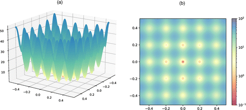
Notes. (a) Contour plot. (b) Heatmap of function values.
We compared ε-greedy against the methods of Regis and Shoemaker (2005) and Regis and Shoemaker (2007) on this function. Both methods (referred to, respectively, as RS05 and RS07) are based on RBF interpolation, and thus are natural benchmarks for the framework of this paper. For context, we note that the extensive computational study in Regis and Shoemaker (2007) does not consider any problem with more than 6 dimensions. Thus, the 30-dimensional Rastrigin function is a very large and difficult problem by the standards of this literature.
All three methods were implemented with the Gaussian kernel . The RBF interpolant was constructed as laid out in Section 3, but for simplicity we did not use any polynomial components. All three methods were initialized using a single point uniformly sampled on the domain; the initialization strategies used by RS05 and RS07 as originally proposed are not practical in 30 dimensions because they would require too many points. All three methods were also allowed to use the well-known practical strategy, dating back to Björkman and Holmström (2000), of replacing large function values by the median of all sampled values. Finally, all three methods used the same subroutine, based on trust-region optimization (chapter 14 of Conn et al. 2000), for computing the minimizer of .
We made some adjustments to the benchmarks to make their computational cost roughly comparable to that of ε-greedy (to the extent possible). In every iteration, RS07 chooses from a certain number of points generated uniformly at random. This number is set to 1,000d in the method as originally proposed, but that is obviously not practical in 30 dimensions, so we used 2,250 samples per iteration instead. RS05 solves two auxiliary optimization problems on a discretization of the domain; we used 1,000 points in the discretization. The settings of ε-greedy were set to cr = 50, k = 50, and b = 0.3.
The focus of our theoretical study is the metric . This metric, averaged over 10 runs, is reported in Figure 2(a) with 95% confidence intervals for up to n = 600 function evaluations. We see that, by the end of this time frame, ε-greedy is much more effective at estimating the location of the global minimizer. RS05 is marginally better up to about n = 320 but then slows down. RS07 never really improves on its initial estimate.

Notes. (a) . (b) Log-scaled time cost (seconds) per iteration. (c) . (d) .
To better understand what is happening, let be the best among the first N points observed. Figure 2(c) reports , a measure of the quality of the observed points. Because ε-greedy chooses many points uniformly at random, one would not expect it to do well under this metric. Yet, by n = 600, we find some overlap between the CIs for all three methods, indicating that ε-greedy has largely caught up with the benchmarks. One can also improve the result for ε-greedy by increasing the probability of global search, though this will make the primary metric worse.
Figure 2(d) reports . Here we see very clearly that RS07 is actually moving away from over time, toward a local optimum that is producing seemingly low values of . RS05 gets stuck at a local optimum very early on (also seen in Figure 2(c)) but is actually building a more accurate RBF model with the points it samples, explaining the improvement in Figure 2(a). The wide CIs seen in Figure 2(c) for RS05 are due to the instability of the auxiliary problem solved by this procedure; because RS05 is stuck after approximately 50 iterations, the confidence bounds do not shrink.
Figure 2(b) shows that all three methods incur higher computational cost over time, which is to be expected because the complexity of the RBF model increases with the number of design points. There is some fluctuation in the cost (most notably for RS05) because of the numerical instability of the auxiliary optimization problems solved by the methods. Overall, ε-greedy and RS07 have roughly similar cost, whereas RS05 is significantly slower.
In conclusion, ε-greedy shows itself to be more effective in estimating the global minimizer than the two benchmarks. At the same time, it takes longer to find a good solution, as measured by . In our experience, the tradeoff between these goals can be tuned using the parameter b. Of course, we do not claim that such a simple algorithm as ε-greedy will “always” outperform two of the leading computational benchmarks in the field. Rather, the conclusion that should be drawn is that there are certain settings where even the most sophisticated methods will struggle, and very competitive performance can then be obtained from very simple algorithms.
6. Proof of Theorem 1
We now move to the proofs of the main results of our paper. The pathwise rate in Theorem 1 can be obtained once is in a neighborhood of the global optimum, in which we can make use of the local strong convexity of f. Thus, the proof of the theorem consists of two parts. Section 6.1 proves that will remain in this neighborhood for all sufficiently large N. Then, in Section 6.2 we can assume that and study the convergence rate.
6.1. Convergence of to a Neighborhood of
The main goal in this section is to prove
Our analysis proceeds by deriving a lower bound on . This bound will eventually be shown to converge to 1. Similarly to the proof of Lemma 4, we rewrite the distribution of xn as follows. For any n, let be a latent variable; then, if zn = 1, draw , and if zn = 0, draw xn from a distribution with density , where gn is as in (3). We then denote by the subset of the design points coming from the uniform density, with being the number of such samples.
The first step in the proof, stated in the following technical lemma, is to bound the probability of interest by the sum of two more tractable probabilities, which will also be bounded in subsequent steps. The proof is moved to the Appendix.
Define and
The next lemma, whose proof is also moved to the Appendix, bounds the first term on the right-hand side of (8). After that, in Lemma 8, we will bound the second term and combine this with the result of Lemma 7 to complete the proof of the theorem.
Let cw be the constant obtained from Lemma 6. There exists another positive constant such that
There exists a positive constant such that
Let and be as in the statement of Lemma 6. We calculate
Taking the expectation over the distribution of NU, we obtain
By the independence of , we obtain
Then,
Combining (9) with Lemmas 6 and 7, we obtain
whence the desired result follows. □
From Lemma 8, it follows that
We then obtain (7) by a direct application of the Borel-Cantelli lemma.
6.2. Convergence Rate Around
From the preceding, we know that there is an a.s. finite random number such that whenever . Other than this, we will not refer to any result from Section 6.1. The flow of the proof is somewhat complicated; the relationships between various intermediate steps are given in Figure 3. However, one can think of the proof as consisting of two major tasks. The first task is to prove a rate on inside the ball . In Figure 3, the end result of this task is represented by (17), and the components that lead into it in the diagram represent intermediate results mainly focusing on the properties of the Hessian of f obtained from local strong convexity.

The second task, represented in Figure 3 by Lemma 10 and (18), improves on the rate obtained from the first task by showing more explicitly how it depends on the local search radius rn. Theorem 1 is then concluded by setting rn as indicated in (5).
We now begin the first task. Keeping the notation introduced previously, we begin by applying the strong law of large numbers to NU. Because
Then,
almost surely as .
Our immediate goal now is to relate to , thus yielding a rate through (10). This connection can be made through the function f, because applying Lemma 1 on gives
and
We will now work to connect these results to using a second-order Taylor expansion. Letting and be the Hessian matrices of (respectively) f and at x, we can write
for some on the segment joining and , that is,
Similarly, we have
for some on the segment joining and . Adding (11) and (12), we obtain the upper bound
A lower bound involving can be obtained via
The constant
satisfies by the assumption that f is locally strongly convex inside . A further lower bound can be obtained from the following technical lemma (whose proof is deferred to the Appendix).
For a positive definite d × d matrix A satisfying for all i, j, then .
Applying Lemma 9 to (14) leads to
Combining (13) with (15) yields
almost surely when and is small enough. Considering the decreasing rate of the mesh norm obtained from (10), this in turn implies
The rate in (17) can be improved by narrowing the local search region over time, as long as both and are elements of each region in the sequence, and we collect infinitely many samples from these regions. The decay rate of begins to play an important role in ensuring that these conditions hold. If rn decays too slowly, we will undersample in the local regions; if rn decays too quickly, our local regions may fail to cover .
It turns out that the best possible rate for rn is for some large enough constant . With this specific choice, the following result is obtained.
Suppose that xn is sampled from the density gn defined in (3). Let for and define
almost surely.
We have already obtained (17). From this result, there exist a constant cb and an integer nr such that, for all ,
Let cr be large enough to satisfy, uniformly over the possible values of nr, the inequality
Then, we have a.s., whence and . Similarly, for all n, N satisfying , we have a.s., whence we obtain , as required. □
From Lemma 10, it follows that the ball
From (3), we have a.s. for all and . Let
Any was drawn from a uniform distribution on BN. The volume of BN satisfies
for some constant cB.
Conditional on , take and let be independent Bernoulli random variables, with the success probability of being for . Sampling xn from the density gn is equivalent to sampling uniformly on BN if , and sampling from a distribution with density function if . Then, because , it follows by the strong law of large numbers and the a.s. finiteness of that
Note that BN is shape-regular because we can use a shifting and scaling mapping on into BN. The scaling factor is precisely . The mesh norm of a set will be invariant if is translated and the sampling density is changed accordingly. If is scaled isotropically and the sampling density is changed accordingly, the mesh norm will be scaled by the same scaling factor.
Conditional on contains points sampled uniformly on BN. By Lemma 4 and the properties of the bijection obtained from shape regularity, we have
Because when , with almost surely, we can obtain the a.s. inequality
Recall that , and observe that as . It follows, analogously to (17), that
With , the rate of tN follows from (4), and is given by
From this it follows that
which means that , as required. Finally, substituting (20) into (19) yields
as claimed by Theorem 1.
Equation (19) illustrates the benefit of shrinking rN. If the size of the local search region is constant (i.e., ), we can see that tN will also be a constant, and the convergence rate will reduce to (17). The bound is tightened when tN becomes larger, with the tightest bound obtained when rN follows (5). At the same time, we cannot make rN vanish more quickly than the rate obtained in (17) using the properties of the mesh norm.
7. Proof of Theorem 2
The flow of the proof is quite complicated and requires many interlocking parts, whose relationships are illustrated in Figure 4. Three main tasks, corresponding to Sections 7.1 to 7.3, can be identified:
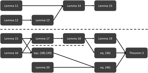
In Section 7.1, the main goal is to derive a concentration inequality for the mesh norm defined on under uniform sampling. This task is represented by the top part of Figure 4, above the first dashed line. The analysis is self-contained; only the final result, stated in Lemma 15, is used for subsequent tasks.
In Section 7.2, we then derive a similar concentration inequality for the mesh norm, but this time on a general domain and under ε-greedy sampling. The final result, shown in Figure 4 above the second dashed line, is Lemma 18.
Finally, in Section 7.3, the concentration inequalities obtained for the mesh norm are converted into analogous results for the estimation error , arriving at Theorem 2.
7.1. Concentration of Mesh Norm on Under Uniform Sampling
In this section, we derive a concentration inequality on the mesh norm with being a set of N uniformly sampled design points. Specifically, we bound the probability that, at a fixed time N, the mesh norm does not yet obey the asymptotic pathwise rate obtained from Lemma 3.
To study the behavior of the mesh norm in finite time, we partition the domain into a finite number of subsets, then grow the size of the partition as more design points are sampled at a suitably chosen rate. The growth rate of the partition size can be related to the declining behavior of the mesh norm. This analysis is based on combinatorics and largely self-contained, with only the final result being used in further tasks.
Specifically, we consider sets of the form with for . We then have and has zero Lebesgue measure for any (also under the measure induced by the uniform distribution). Each subset also has the same volume under either measure.
Given N design points, let M be the maximum number of subsets into which the domain can be partitioned (according to the method described previously) such that each subset contains at least one design point in its interior. The probability that any design points will fall exactly on the joint boundary of two adjacent subsets is zero. Formally,
Thus, M is a random variable that takes positive integer values and is dependent on N. We are interested in the increasing rate of M as N becomes large.
First, for fixed positive integers m and N, let be a random vector following a multinomial distribution with parameters (N, m) and probability vector , where for each component j. The following result (proved in the Appendix) calculates the probability that no subsets will be empty.
For any N and m,
Now observe that
because the maximum partition size is at least m if and only if, in the partition whose size is m, each subset contains at least one design point. In another way of writing, , where represents a Stirling number of the second kind, defined for general m, n as
By following the asymptotic analysis of Stirling numbers (Temme 1993), we can obtain the following increasing rate of M. The next result (whose proof is deferred to the Appendix) then derives a more useful equivalent form for this approximation.
(Temme 1993). The Stirling number of the second kind can be approximated (uniformly in m, and asymptotically as ) as
and y0 is the solution of .
The Stirling number of the second kind can be approximated (uniformly in m, and asymptotically as ) as
Now, we can apply Lemma 13 to obtain an asymptotic rate for that is expressible in closed form as a function of N and m. Consequently, as N grows large, we can choose a suitable growth rate for m that would allow us to achieve a partition of size m w.p.1. The following bound (proved in the Appendix) provides a sufficient condition for this growth rate to be suitable.
If and with , then for some constant .
With these technical results, we return to the decreasing rate of the mesh norm on under uniform sampling. The final result of this section follows fairly straightforwardly from the preceding.
Let be a set of N design points sampled independently from the uniform distribution on . There exist constants such that, for any n > 1,
There exists a constant such that the statement (for any m) implies that . To match the almost sure convergence rate of the mesh norm, choose . Then, there exist constants such that, for any N > 1,
7.2. Concentration of Mesh Norm on Under ε-Greedy Sampling
The final result of this section is an analog of Lemma 15 from the previous section with the general domain and the design points obtained from ε-greedy sampling. We move to this more general case in two steps. First, we consider nonuniform sampling while keeping the domain as , and then extend the result to a general domain.
Let where each is sampled independently from a density with support . Let and suppose that and as . Let be independent Bernoulli random variables with success probabilities so that, if , then is sampled from a uniform distribution on , and if , then is sampled from the density .
Let and . A direct application of Hoeffding’s inequality yields
In later proofs, this will be combined with the following technical result (proved in the Appendix).
If , then
With the previous preliminaries, we may establish the following concentration inequality for the mesh norm on under nonuniform sampling. The main idea is to apply Lemma 15 to the part of the data that comes from a uniform distribution.
There exist constants such that, for large enough N,
For notational compactness, denote the event
For any arbitrary positive value of , we derive
where (25) is due to Lemma 16 and (24).
When N satisfies
where (26) applies Lemma 15 to (25), and is suitably chosen to dominate the second term in (26). □
The concentration inequality can now be generalized to the domain . Because we assume that is shape regular, there exists a continuously differentiable bijection whose Jacobian has nonzero determinant everywhere on its domain. The proof works with the inverse image of under , similar to the proof of Lemma 5.
There exist constants such that, for all large enough N,
As in the proof of Lemma 5, we observe that the mapping is Lipschitz. The Lipschitz condition implies
For each n, define a density
Then, letting , we have , where . We also have , where .
For any arbitrary positive value of , the inequalities
Now choose , where is the constant obtained from Lemma 17. It follows that, for all N satisfying (28), we have
where is the constant obtained from Lemma 17. Letting yields the desired result. □
If the Inequality (27) holds for a certain value of , it also holds for any larger value. The same is true of the other concentration inequalities on the mesh norm that we derived throughout this section.
7.3. Concentration Inequality for Estimation Error
Finally, we connect the previously obtained results for the mesh norm to the estimation error . We first take care of the situation where is converging to too slowly, by deriving a bound on the probability of this event. This is done by building on Lemma 8.
Then, conditional on the event , we apply (16), which implies the existence of a constant such that, for all N,
At this point, Lemma 18 provides a probabilistic bound for the right-hand side of (29). We thus obtain the following concentration inequality on , although it is still not the strongest one possible because the right-hand side of (29) only considers a ball with fixed radius. The situation is analogous to Section 6.2, where we also first derived a rate within that ball, and later improved it by incorporating the shrinking radius.
There exist constants such that, for all large enough N,
We derive
where in (30) is the same value as in (29). Now, if we choose , where is the same as in Lemma 18, we obtain
where is the same as in Lemma 18. The desired result follows. □
Now, analogously to Section 6.2, we will strengthen this result by considering the local search radius rn set according to (5) with some sufficiently large cr. We first show that, using such a radius, the local sampling regions for will cover
Before we proceed, we slightly relax the constant in Lemma 18. From (10), we have
for all large enough N (the exact threshold value of N at which this happens may be random, however). Thus, we can let and replace in Lemma 18 by without changing the result. Similarly, if N is large enough for (32) to hold, then we will still have Inequality (32) if we replace by .
Now, consider the set of the first n data points. We observe that is decreasing in n. Thus, if and for some , then
where are as in (31). It follows that the number of time stages in which SN is covered by is bounded below by the number of times that
is achieved.
The remainder of our analysis is based on this concept of coverage. Whenever SN is covered by , there is a certain probability (varying with n) that a sample drawn from the local search region falls in SN. Recalling that the ε-greedy algorithm conducts local search by sampling uniformly inside the local region, one can then interpret the distribution of that sample as a mixture of uniforms. In other words, whenever SN is contained in the local search region, there is a certain probability that the sample will be drawn from a uniform distribution on SN. One can then make use of Lemma 15 to study the convergence rate of the mesh norm in SN, a neighborhood of the global optimum.
To make these arguments, we first need to ensure that coverage occurs, that is, the probability that SN is never covered in the above-described manner is sufficiently small. Let n be some fixed integer large enough to satisfy Inequality (28) and define
holds almost surely. We will discard a suitable set of measure zero from the outcome space so that (35) can be assumed to always hold, and we do not have to keep conditioning on this event in our analysis.
With this, let be a fixed value satisfying (28). Then,
Now, we study the portion of the design points that can be viewed as originating from a uniform distribution on SN. Let , for , be independent Bernoulli random variables with success probabilities . Then, is the cardinality of the subset of the data that was sampled uniformly on SN. Note that and are independent. We introduce the notation nk, for , to represent those time stages for which , that is,
Recall from Lemma 15 that, if is a set of independent and identically distributed (i.i.d.) samples from the uniform density on , then
for notational convenience, we then have
Recall from (20) that . Now, we define
and repeat the proof of Lemma 16 to obtain the inequality
under the condition that . This allows us to improve the lower bound on in the event whose probability is computed in (38) to match the asymptotic a.s. rate of . The resulting inequality can then be directly connected to the estimation error.
First, we give a technical lemma characterizing the probability that the condition required for (39) is not satisfied.
The following statement holds:
Conditional on is a sum of independent Bernoulli random variables. Applying Hoeffding’s concentration inequality, we derive
Provided that and , the inequality implies that , whence, applying (20), we obtain
whence and . Therefore,
Because and NS are all strictly positive random variables when , we can apply Fatou’s lemma to obtain
which yields a further bound on (40) because of the relation
for any N satisfying (28). This completes the proof. □
Now, letting , where ch is the value obtained from (38), and also letting for notational convenience, we can derive
We then derive the bound
In this derivation, (44) is obtained by applying (42) to the first term of (43), and Lemma 20 to the second term. Then, (45) is due to (38).
By repeating the proof of Lemma 20, we can derive
Similarly to (19), when , we can bound the error of by the local mesh norm on SN as
It follows from the preceding that there exists a constant such that
Using the fact that and , there exists a constant such that
shown by applying Lemma 19 together with (36) and (46). By combining this bound with the preceding analysis on the rate of tN, we obtain constants for which
for all N satisfying (28). This condition on N depends only on b and the constant cJ, which itself depends only on the domain and not on f.
8. Conclusion
We presented new convergence rate results for global optimization using radial basis function interpolation and an ε-greedy algorithm that randomly chooses between uniform sampling on the entire domain versus uniform sampling on a local neighborhood of the current estimated minimizer. This sampling method is simple to implement but captures the key distinction between local and global search that is present in many other algorithms that are not amenable to theoretical analysis. We find that convergence rates are improved when the size of the local search region is made to shrink over time at a suitable rate, that is, local search concentrates around the estimated minimizer over time.
The theory of RBF interpolation relies on a bound connecting the interpolation error to the distribution of the design points on the domain. The overall structure of our proof could potentially be repeated for other interpolation models as long as those models also had bounds of this kind (not necessarily the same order) available. The bounds improve when the design points are more evenly spread out; thus, although it is possible to obtain very similar rates for the case where global search is conducted using nonuniform sampling, it is not possible to improve the rates using this analytical technique. To obtain such improvements, it would be necessary to develop new theory that makes a closer connection between the error of RBF interpolation and the shape of the underlying function; we leave this problem for future work.
The authors thank the editor-in-chief, associate editor, and two referees for careful reading of the paper and constructive comments.
Appendix A. Proof of Lemma 6
First, observe that if
where .
Inequality (A.1) is implied if
holds for any , ρ satisfying . The sufficient event (A.2) implicitly excludes the situation where no design points are in .
Next, by Lemma 1, for all large enough N and all satisfying , we have
where does not depend on . Thus, the sufficient condition (A.2) is attained if
or, equivalently,
Now, define
On the event , Inequality (A.3) is attained, which, in turn, implies as desired.
Because , we can easily see that , and hence it is sufficient to restrict ourselves to the event . Therefore, we conclude that
as required.
Appendix B. Proof of Lemma 7
By Lemma 5, we have
Therefore, with a probability of one, there exists a random but a.s. finite value such that
It follows that
for any when . Taking , we let , which depends on the random variable , and obtain when .
Consequently,
To bound (B.1), we require a concentration inequality for NU. Note that , where zn are i.i.d. random variables. The expected value of NU increases to infinity with N.
We derive
Using Hoeffding’s concentration inequality, we obtain
whence
as desired.
Appendix C. Proof of Lemma 9
For any vector in ,
The desired result follows by taking the supremum over all nonzero v.
Appendix D. Proof of Lemma 11
We prove this result by induction. When m = 1, it is obviously correct; when m = 2, we have , also according to (21).
Suppose now that (21) holds for . Then,
thus verifying (21) and completing the proof.
Appendix E. Proof of Lemma 13
Let y0 be the solution of the equation , and let . Then, we have
This implies , where . From Lemma 12, we have (22), and we can derive
as required.
Appendix F. Proof of Lemma 14
Let T and τ be as in the statement of Lemma 12, and let w be as in the statement of Lemma 13. Also let . First, we derive
Consider the decreasing rate of the first term on the right-hand side of (F.1). Taking advantage of Stirling’s formula
we derive
where (F.2) is obtained by first using the Lagrange inversion theorem to derive the expansion
for the upper branch W0 of the Lambert W function when and then observing that
for large s.
Now consider the decreasing rate of the second term on the right-hand side of (F.1). Based on Temme (1993), one can show that
whereupon, with some tedious algebra, one finds . Then,
where (F.5) follows by (F.4), Equation (F.6) follows from , and (F.7) follows from (F.3) and the fact that . Because we have found that both terms on the right-hand side of (F.1) are , the desired result follows.
Appendix G. Proof of Lemma 16
For and , we have the inequality
Take and and divide both sides of the inequality by to obtain
which leads to the desired result.
References
- (2006) Convergence of mesh adaptive direct search to second-order stationary points. SIAM J. Optim. 17(2):606–619.Google Scholar
- (2006) Mesh adaptive direct search algorithms for constrained optimization. SIAM J. Optim. 17(1):188–217.Google Scholar
- (2008) Nonsmooth optimization through mesh adaptive direct search and variable neighborhood search. J. Global Optim. 41(2):299–318.Google Scholar
- (2010) A mesh adaptive direct search algorithm for multiobjective optimization. Eur. J. Oper. Res. 204(3):545–556.Google Scholar
- (1996) Evolutionary Algorithms in Theory and Practice: Evolution Strategies, Evolutionary Programming, Genetic Algorithms (Oxford University Press, Oxford, UK).Google Scholar
- (2015) A derivative-free comirror algorithm for convex optimization. Optim. Methods Software 30(4):706–726.Google Scholar
- (2019) Derivative-free optimization of noisy functions via quasi-newton methods. SIAM J. Optim. 29(2):965–993.Google Scholar
- (2000) Global optimization of costly nonconvex functions using radial basis functions. Optim. Engrg. 1(4):373–397.Google Scholar
- (2003) Radial Basis Functions (Cambridge University Press, Cambridge, UK).Google Scholar
- (2011) Convergence rates of efficient global optimization algorithms. J. Machine Learn. Res. 12:2879–2904.Google Scholar
- (2018) On convergence rate of a rectangular partition based global optimization algorithm. J. Global Optim. 71(1):165–191.Google Scholar
- (2000) Trust Region Methods (SIAM, Philadelphia).Google Scholar
- (1997) On the convergence of derivative-free methods for unconstrained optimization. Buhmann MD, Iserles A, eds. Approximation Theory and Optimization: Tributes to M.J.D. Powell (Cambridge University Press, Cambridge, UK), 83–108. Google Scholar
- (2009a) Global convergence of general derivative-free trust-region algorithms to first-and second-order critical points. SIAM J. Optim. 20(1):387–415.Google Scholar
- (2009b) Introduction to Derivative-Free Optimization (SIAM, Philadelphia).Google Scholar
- (1987) Minimizing multimodal functions of continuous variables with the “simulated annealing” algorithm. ACM Trans. Math. Software 13(3):262–280.Google Scholar
- (2015) Optimal rates for zero-order convex optimization: The power of two function evaluations. IEEE Trans. Inform. Theory 61(5):2788–2806.Google Scholar
- (2006) Efficient optimization of support vector machine learning parameters for unbalanced datasets. J. Comput. Appl. Math. 196(2):425–436.Google Scholar
- (2015) Derivative-free methods applied to daily production optimization of gas-lifted oil fields. Comput. Chem. Engrg. 75:60–64.Google Scholar
- (2001) A radial basis function method for global optimization. J. Global Optim. 19(3):201–227.Google Scholar
- (2008) An adaptive radial basis function algorithm (ARBF) for expensive black-box global optimization. J. Global Optim. 41(3):447–464.Google Scholar
- (2004) Recent advances in particle swarm. Proc. 2004 Congress Evolutionary Comput., vol. 1, (IEEE, Piscataway, NJ), 90–97.Google Scholar
- (2006) Sequential kriging optimization using multiple-fidelity evaluations. Structural Multidisciplinary Optim. 32(5):369–382.Google Scholar
- (1987) Maximal spacings in several dimensions. Ann. Probability 15(1):274–280.Google Scholar
- (1998) Efficient global optimization of expensive black-box functions. J. Global Optim. 13(4):455–492.Google Scholar
- (2011) Personalized pricing recommender system: Multi-stage epsilon-greedy approach. Cantador I, Brusilovsky P, Kuflik T, eds. Proc. 2nd Internat. Workshop Inform. Heterogeneity Fusion Recommender Systems (ACM, New York), 57–64.Google Scholar
- (2003) Optimization by direct search: New perspectives on some classical and modern methods. SIAM Rev. 45(3):385–482.Google Scholar
- (1999) Pattern search algorithms for bound constrained minimization. SIAM J. Optim. 9(4):1082–1099.Google Scholar
- (2000) Pattern search methods for linearly constrained minimization. SIAM J. Optim. 10(3):917–941.Google Scholar
- (2002) Finite-time performance analysis of static simulated annealing algorithms. Comput. Optim. Appl. 21(1):21–53.Google Scholar
- (1994) A direct search optimization method that models the objective and constraint functions by linear interpolation. Advances in Optimization and Numerical Analysis (Springer, Berlin), 51–67.Google Scholar
- (2002) UOBYQA: Unconstrained optimization by quadratic approximation. Math. Programming 92(3):555–582.Google Scholar
- (2014) Sequential crowdsourced labeling as an epsilon-greedy exploration in a Markov decision process. Kaski S, Corander J, eds. Proc. 17th Internat. Conf. Artificial Intelligence and Statist., 832–840.Google Scholar
- (2005) Constrained global optimization of expensive black box functions using radial basis functions. J. Global Optim. 31(1):153–171.Google Scholar
- (2007) Improved strategies for radial basis function methods for global optimization. J. Global Optim. 37(1):113–135.Google Scholar
- (2009) Parallel stochastic global optimization using radial basis functions. INFORMS J. Comput. 21(3):411–426.Link, Google Scholar
- (2013) Combining radial basis function surrogates and dynamic coordinate search in high-dimensional expensive black-box optimization. Engrg. Optim. 45(5):529–555.Google Scholar
- (2002) Exploration of metamodeling sampling criteria for constrained global optimization. Engrg. Optim. 34(3):263–278.Google Scholar
- (2005) A study of global optimization using particle swarms. J. Global Optim. 31(1):93–108.Google Scholar
- (2018) ASTRO-DF: A class of adaptive sampling trust-region algorithms for derivative-free stochastic optimization. SIAM J. Optim. 28(4):3145–3176.Google Scholar
- (2008) A new trust region method with adaptive radius. Comput. Optim. Appl. 41(2):225–242.Google Scholar
- (2010) Gaussian process optimization in the bandit setting: No regret and experimental design. Fürnkranz J, Joachims T, eds. Proc. 27th Internat. Conf. Machine Learn. (Omnipress, Madison, WI), 1015–1022.Google Scholar
- (2018) Reinforcement Learning: An Introduction, 2nd ed. (MIT Press, Cambridge, MA).Google Scholar
- (2020) Convergence of Gaussian process regression with estimated hyper-parameters and applications in Bayesian inverse problems. SIAM/ASA J. Uncertainty Quantification 8(4):1310–1337.Google Scholar
- (1993) Asymptotic estimates of Stirling numbers. Stud. Appl. Math. 89(3):233–243.Google Scholar
- (2006) On the Markov homogeneous optimization method. Comput. Math. Math. Phys. 46(3):361–375.Google Scholar
- (1997) On the convergence of pattern search algorithms. SIAM J. Optim. 7(1):1–25.Google Scholar
- (2020) Regret bounds for noise-free Bayesian optimization. Preprint, submitted February 12, https://arxiv.org/abs/2002.05096.Google Scholar
- (2006) A study of particle swarm optimization particle trajectories. Inform. Sci. 176(8):937–971.Google Scholar
- (2007) A particle swarm pattern search method for bound constrained global optimization. J. Global Optim. 39(2):197–219.Google Scholar
- (2010) Pointwise consistency of the kriging predictor with known mean and covariance functions. Advances in Model-Oriented Design and Analysis (Springer, Berlin), 221–228.Google Scholar
- (2011) Global convergence of radial basis function trust region derivative-free algorithms. SIAM J. Optim. 21(3):761–781.Google Scholar
- (2008) ORBIT: Optimization by radial basis function interpolation in trust-regions. SIAM J. Sci. Comput. 30(6):3197–3219.Google Scholar
- (1993) Local error estimates for radial basis function interpolation of scattered data. IMA J. Numerical Anal. 13(1):13–27.Google Scholar
- (2010) Firefly algorithm, Levy flights and global optimization. Bramer M, Ellis R, Petridis M, eds., Research and Development in Intelligent Systems, vol. 26 (Springer, London), 209–218.Google Scholar
- (2008) Stochastic Global Optimization (Springer, Berlin).Google Scholar