Large-Time Behavior of Finite-State Mean-Field Systems With Multiclasses

1. Introduction

Interacting particle systems with multiclasses, widely encountered in a variety of domains going from statistical physics, chemistry, communication networks, and biology to finance, have recently attracted the interest of many researchers, and several models have been proposed to understand their large-scale behavior. See, for example, Graham (2008), Collet (2014), Collet et al. (2016), Chong and Klüppelberg (2019), Knöpfel et al. (2020), Meylahn (2020), and Nguyen et al. (2020) and the references therein for an overview of recent advances on the subject. In multiclass systems, the particles come from different subpopulations, within which they are homogeneous, and thus, the entire system is heterogeneous but composed of homogeneous subpopulations. Thence, one can average over the local symmetries within the different classes to describe mean-field interactions through local empirical measures. Thus, the entire system is characterized by an empirical vector composed of the local empirical measures.

The focus of the current article is on a particular family of mean-field multiclass models describing the evolution of block-structured networks with dynamically changing multicolor nodes. The state-space here is a finite set of colors, and the particles are identified as the nodes of the network. This class of models was proposed in Dawson et al. (2020) to describe the dynamic of various physical phenomena, and the large-scale asymptotics were established. In particular, a multiclass propagation of chaos was proven to hold together with a law of large numbers, implying the convergence of the empirical vector toward the solution to a McKean-Vlasov system of equations as the total number of particles N in the system goes to infinity. Moreover, these authors studied the large deviations principle for the empirical vector process over finite time intervals.

We propose in this article to study the large-time behavior of the family of models introduced in Dawson et al. (2020). Our motivation comes from the interesting characteristics of these systems as well as the importance of their large-time behavior for many applications. Notice that numerous works on the large-time behavior of various systems of interacting particles exist in the literature. See, for example, Cox and Greven (1990), Dawson and Greven (1993; 1999), Dawson et al. (1995), Greven and den Hollander (2007), Döring and Mytnik (2013), and Kuehn (2015) and references therein. Therefore, our current contribution aims to be the continuation of the aforementioned references. The approach taken in this document is summarized as follows.

First of all, let us mention that the propagation of chaos and the law of large numbers established in Dawson et al. (2020) are valid over finite time intervals. Thence, on any finite time horizon (not too large), one could use the McKean-Vlasov limit system as an approximation for the large N-particle system because it is classical in the mean-field literature. However, when time tends to infinity, these results are no longer necessarily true, and care should be taken in using this approximation. Indeed, as we detail throughout this article, the validity of the approximation is intimately linked to the critical points of the McKean-Vlasov limit system and its stability. Intuitively, if the McKean-Vlasov limit system has several ω-limit sets, one can wonder which of these sets characterizes the large-time behavior of the large N-particle system.

As a starting point to tackle this problem, we study in Section 4 the asymptotics of the invariant measure of the empirical vector. In particular, we establish, under mild conditions, the large deviations principles for the invariant measure in two different cases, first when there exists a unique asymptotically stable equilibrium to the McKean-Vlasov system (Theorem 4) and then when the McKean-Vlasov system has multiple ω-limit sets (Theorem 5). More precisely, Theorem 4 states that when the McKean-Vlasov system has a unique globally asymptotically stable equilibrium ξ₀, the value at a given state ξ of the rate function that governs the large deviations principle of the invariant measure is given by the minimum cost of transporting the system state from the globally asymptotically stable equilibrium ξ₀ to ξ across all the possible paths in any time duration. Theorem 5 gives a generalization to the case where the McKean-Vlasov system has multiple ω-limit sets. To this end, one relies on the classical hypothesis of Friedlin and Wentzell (2012). Note that the large deviations principles of the invariant distribution have been established for interacting diffusions in Dawson and Gärtner (1989) and for finite-state mean-field systems on complete graphs in Borkar and Sundaresan (2012). We adopt here the control theory approach introduced in Biswas and Borkar (2011) for small noise diffusions and extended in Borkar and Sundaresan (2012) to interacting jump processes on complete graphs. Therefore, we further extend this approach to the heterogeneous case with block-structured interaction graphs.

Next, we investigate the metastable phenomena, in the sense of Friedlin and Wentzell’s (2012) small noise stochastic systems, emerging when the McKean-Vlasov limiting system has several ω-sets. Namely, in the case of multiple attractors, the empirical vector process, which is associated with a large but finite number of particles N, would transit between these attractors when the time is large. One then aims to estimate the most probable order in which these transitions occur and the average time spent in the neighborhood of each of the ω-limit sets. Understanding these phenomena is of great practical interest, and hence, our motivation. We describe in Section 5 the metastable phenomena in more detail and give important estimates. For this, we adopt the classical approaches of Freidlin and Wentzell (2012, chapter 6) and Hwang and Sheu (1990). The main ingredients are the large deviation properties of the empirical vector process over finite time periods established in Section 3, and the main tool is the Freidlin-Wentzell quasipotential derived from the rate function characterizing the large deviations principle. Subsequently, we develop in Theorem 7 an estimate of the time required for the empirical vector process to converge to its invariant measure. We find out that when the time is of the order $\exp \{N(\mathrm{\Lambda }+\delta )\}$, for all $\delta >0$ and $\mathrm{\Lambda }$ being an appropriate constant, the empirical vector process is very close to its invariant measure. Interestingly, this coincides with the timescale found in Hwang and Sheu (1990) for diffusion processes and in Borkar and Sundaresan (2012) for finite-state mean-field systems on complete graphs. We underline that the metastable phenomena in the Section 5 are studied under Assumption 2. Note, however, that if these assumptions are not imposed, things are more complicated, and this is not pursued here. The reader may consult Zhou et al. (2012), Bouchet et al. (2016), and Tang et al. (2017) and the references therein for discussions and examples.

It is worthwhile to mention that, although the methodology used in the current work follows the one in Borkar and Sundaresan (2012) and Yasodharan and Sundaresan (2019) based on the small-noise large deviations of diffusion processes introduced in Hwang and Sheu (1990) and Freidlin and Wentzell (2012), we emphasize that our results are established for empirical vectors and thus on product spaces. In particular, the multiclass structure of the system breaks down the homogeneity and global interaction hypothesis made in Borkar and Sundaresan (2012) and Yasodharan and Sundaresan (2019). Thus, one cannot directly rely on the results obtained in Borkar and Sundaresan (2012) and Yasodharan and Sundaresan (2019) because the global empirical measures in our current model are not expected to satisfy the law of large numbers, nor is the large deviations principle established for the global empirical measure. Our strategy to overcome the difficulties arising from the heterogeneity is through a finer-grain analysis of each local empirical measure describing each subclass.

The rest of this paper is organized as follows. In Section 2, we revisit the family of models introduced in Dawson et al. (2020). One may also consult Dawson et al. (2020; section 2) for a full detailed description together with some examples. Section 3 is dedicated to the large deviations properties of the empirical vector process over finite time intervals. We first recall the principal results of Dawson et al. (2020) and then introduce some additional results used in the following sections. Then, we prove in Section 4 our first set of the main results. Namely, Theorem 4 gives the large deviations principle for the empirical measures when the McKean-Vlasov system has a unique globally asymptotically stable equilibrium, and Theorem 5 gives the large deviations principle of the invariant measure when there are multiple ω-limit sets. In addition, we recall some important concepts from the Friedlin-Wentzell large deviations theory. We then investigate in Section 5 the metastability of the N-particles system. Based on a set of results, we provide estimates of the metastable transitions. Finally, Theorem 7 gives the time required for the empirical vector process to converge toward its invariant measure.

Because the results of Sections 4 and 5 rely on the Freidlin-Wentzell program described in Freidlin and Wentzell (2012, chapter 6), we give in Appendix A the generalization of some of these results to our current setting. Finally, to facilitate the reading, we leave the lengthy proofs of some technical results in Appendix B.

2. The Setting

Consider a graph $\mathcal{G}=(\mathcal{V},\mathrm{\Xi })$ composed of r blocks $C_1,\dots ,C_r$ of sizes $N_1,\dots ,N_r$, respectively, where $\mathcal{V}$ is the set of the nodes and Ξ is the set of the edges. Denote by $\left|\mathcal{V}\right|=N_1+\cdots +N_r=N$ the total number of the nodes in the network. Moreover, suppose that each block C_j is a clique, that is, all the N_j nodes of the same block are connected. We divide the nodes of each block C_j into two sets:

• The central nodes $C_j^c$: connected to all the other nodes of the same block but not to any node from the other blocks. We set $\left|C_j^c\right|=N_j^c$.

• The peripheral nodes $C_j^p$: connected to all the other nodes of the same block and all the peripheral nodes of the other blocks. We set $\left|C_j^p\right|=N_j^p$.

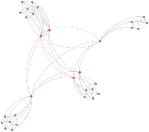
Also, we denote by N^c (resp. N^p) the total number of central (resp. peripheral) nodes in the graph. Notice that an example of such a graph is shown in Figure 1. Let $\mathcal{Z}=\{1,2,\dots ,K\}\subset \mathbb{N}$ be a finite set of K colors. Suppose that each node of the graph $\mathcal{G}=(\mathcal{V},\mathrm{\Xi })$ is colored by one of the K colors at each time. For each $1\le j\le r$ and $n\in C_j^c$ (resp. $n\in C_j^p$), denote by $(X_n(t),t\ge 0)$ the stochastic jump process that describes the evolution of the color of the node n through time. Let $(\mathcal{Z},\mathcal{E})$ be the directed graph where $\mathcal{E}\subset \mathcal{Z}\times \mathcal{Z}\backslash \{(z,z)|z\in \mathcal{Z}\}$ describes the set of admissible jumps. In addition, whenever $(z,z^{\prime })\in \mathcal{E}$, a node colored by z is allowed to jump from z to $z^{\prime }$ at a rate that depends on the current state of the node and the state of its neighbors (adjacent nodes). To characterize these neighborhoods, we introduce, for each block $1\le j\le r$, the following local empirical measures describing, respectively, the state of the central and the peripheral nodes of the j-th block at time t,

and taking values in the set ${\mathcal{M}}_1(\mathcal{Z})$ of probability measures over $\mathcal{Z}$, endowed with the topology of weak convergence. The random dynamic in each block $1\le j\le r$ is thus summarized as follows:

• The central nodes dynamic: Each central node $n\in C_j^c$ jumps from color z to $z^{\prime }$, with $(z,z^{\prime })\in (\mathcal{Z},\mathcal{E})$, at rate

  $${\lambda }_{z,z^{\prime }}^c({\mu }_j^{c,N}(t),{\mu }_j^{p,N}(t)),$$(2.2)
  which depends on its current state and the states of its neighbors through the empirical measures ${\mu }_j^{c,N}(t)$ and ${\mu }_j^{p,N}(t)$.

• The peripheral nodes dynamic: Each peripheral node $n\in C_j^p$ jumps from color z to $z^{\prime }$, with $(z,z^{\prime })\in (\mathcal{Z},\mathcal{E})$, at rate

  $$\begin{array}{l}{\lambda }_{z,z^{\prime }}^p({\mu }_j^{c,N}(t),{\mu }_1^{p,N}(t),\dots ,{\mu }_r^{p,N}(t)),\hfill \end{array}$$(2.3)
  which depends on its state and the states of its neighbors through the local empirical measures ${\mu }_j^{c,N}(t),{\mu }_1^{p,N}(t),\dots ,{\mu }_r^{p,N}(t)$.

Remark 1.

Notice that the rate functions ${\lambda }_{z,z^{\prime }}^c$ and ${\lambda }_{z,z^{\prime }}^p$ depend on the number of nodes $N_j^c$ and $N_j^p$ within each category, but we omit this dependency to not overload the notations, because they do not play a direct role in the study conducted in this paper. In particular, the dependency is not only through the empirical measures ${\mu }_j^{c,N}$ and ${\mu }_j^{p,N}$ but also through the proportions of nodes of the different categories. For example, one possible dependency is described in Dawson et al. (2020) where we suppose the existence of some measurable functions ${\gamma }_{z,z^{\prime }}^{j,c}:\mathcal{Z}\to {\mathbb{R}}^{+}$ and ${\gamma }_{z,z^{\prime }}^{j,p}:\mathcal{Z}\to {\mathbb{R}}^{+}$ such that

• For any probability measures $\nu ,\mu \in {\mathcal{M}}_1(\mathcal{Z})$ and any real numbers $0<a_1,a_2<1$ with $a_1+a_2=1$,

  $${\lambda }_{z,z^{\prime }}^{j,c}(\nu ,\mu ,a_1,a_2)=a_1{\displaystyle {\int }_{\mathcal{Z}}{\gamma }_{z,z^{\prime }}^{j,c}}(x)\nu (dx)+a_2{\displaystyle {\int }_{\mathcal{Z}}{\gamma }_{z,z^{\prime }}^{j,p}}(x)\mu (dx).$$

• For any $\nu ,{\mu }_1,\dots ,{\mu }_r\in {\mathcal{M}}_1(\mathcal{Z})$ and any real numbers $0<a,b_1,\dots ,b_r<1$ such that $a+b_1+\cdots +b_r=1$,

  $${\lambda }_{z,z^{\prime }}^{j,p}(\nu ,{\mu }_1,\dots ,{\mu }_r,a,b_1,\dots ,b_r)=a{\displaystyle {\int }_{\mathcal{Z}}{\gamma }_{z,z^{\prime }}^{j,c}}(x)\nu (dx)+b_1{\displaystyle {\int }_{\mathcal{Z}}{\gamma }_{z,z^{\prime }}^{j,p}}(x){\mu }_1(dx)+\cdots +b_r{\displaystyle {\int }_{\mathcal{Z}}{\gamma }_{z,z^{\prime }}^{j,p}}(x){\mu }_r(dx).$$

In such a case, the rate functions write as

$${\lambda }_{z,z^{\prime }}^{j,c}\left({\mu }_j^{c,N}(t),{\mu }_j^{p,N}(t),\frac{N_j^c}{N_j},\frac{N_j^p}{N_j}\right)=\frac{N_j^c}{N_j}\frac{1}{N_j^c}{\displaystyle \sum _{n\in C_j^c}{\gamma }_{z,z^{\prime }}^{j,c}}(X_n(t))+\frac{N_j^p}{N_j}\frac{1}{N_j^p}{\displaystyle \sum _{n\in C_j^p}{\gamma }_{z,z^{\prime }}^{j,p}}(X_n(t)),$$

and

$$\begin{array}{l}{\lambda }_{z,z^{\prime }}^{j,p}\left({\mu }_j^{c,N}(t),{\mu }_1^{p,N}(t),\dots ,{\mu }_r^{p,N}(t),\frac{N_j^c}{N_j^c+N^p},\frac{N_1^p}{N_j^c+N^p},\dots ,\frac{N_r^p}{N_j^c+N^p}\right)\\ =\frac{N_j^c}{N_j^c+N^p}\frac{1}{N_j^c}{\displaystyle \sum _{n\in C_j^c}{\gamma }_{z,z^{\prime }}^{j,c}}(X_n(t))+\frac{N_1^p}{N_j^c+N^p}\frac{1}{N_1^p}{\displaystyle \sum _{n\in C_1^p}{\gamma }_{z,z^{\prime }}^{1,p}}(X_n(t))+\cdots +\frac{N_r^p}{N_c^j+N^p}\frac{1}{N_r^p}{\displaystyle \sum _{n\in C_r^p}{\gamma }_{z,z^{\prime }}^{r,p}}(X_n(t)).\end{array}$$

We make the following assumptions throughout the paper.

Assumption 1.

1. The directed graph $(\mathcal{Z},\mathcal{E})$ is irreducible.

2. The rate functions ${\lambda }_{z,z^{\prime }}^c$ and ${\lambda }_{z,z^{\prime }}^p$ are Lipschitz and uniformly bounded away from zero, that is, there exists c > 0 such that for all $(z,z^{\prime })\in \mathcal{E},\hspace{0.17em}{\lambda }_{z,z^{\prime }}^c(·)\ge c$ and ${\lambda }_{z,z^{\prime }}^p(·)\ge c$.

3. For each block $1\le j\le r$, there exist $p_j^c,p_j^p,{\alpha }_j\in (0,1)$ such that, as $N\to \infty$,

   $$\frac{N_j}{N}\to {\alpha }_j,\hspace{1em}\frac{N_j^p}{N_j}\to p_j^p,\hspace{1em}\frac{N_j^c}{N_j}\to p_j^c,\hspace{1em}{p}_j^p+p_j^c=1,\hspace{1em}\mathit{\text{ and}}\hspace{1em}{\displaystyle \sum _j{\alpha }_j}=1.$$(2.4)

Remark 2.

Given the compactness of the state-space $\mathcal{Z}$, the space ${\mathcal{M}}_1(\mathcal{Z})$ of probability measures over $\mathcal{Z}$ is also compact by Prokhorov’s theorem. Therefore, the rate functions ${\lambda }_{z,z^{\prime }}^c$ and ${\lambda }_{z,z^{\prime }}^p$ are continuous because Lipschitz, and uniformly bounded from above, that is, there exists a constant $C<\infty$ such that for all $(z,z^{\prime })\in \mathcal{E}$, we have ${\lambda }_{z,z^{\prime }}^c(·)\le C$ and ${\lambda }_{z,z^{\prime }}^p(·)\le C$.

3. Large Deviations of the Empirical Measures

This section gathers large deviations results of the empirical vector process over finite time intervals. We start by introducing some additional notations that will be used in the sequel. Denote by $\mathcal{D}([0,T],\mathcal{Z})$ the Skorokhod space of càdlàg functions defined on $[0,T]$ with values in $\mathcal{Z}$ and by ${\mathcal{M}}_1(\mathcal{D}([0,T],\mathcal{Z}))$ the set of the probability measures over it. Denoting by $X^N=(X_n,X_m,n\in C_j^c,m\in C_j^p,1\le j\le N)\in \mathcal{D}([0,T],{\mathcal{Z}}^N)$ the full description of the N particles over the finite time interval $[0,T]$, we let $M^N\in {\left({\mathcal{M}}_1(\mathcal{D}([0,T],\mathcal{Z}))\right)}^{2r}$ be the vector of “historical” empirical measures defined by

where $M_j^{c,N}$ (resp. $M_j^{p,N}$) is the historical empirical measure of the central (resp. peripheral) nodes of the j-th block. With a slight abuse of notations, denote by G_N the mapping that takes the full description X^N to the empirical measures vector M^N, that is,

Thus, $M^N=G_N(X^N)$. Denote by ${\mathbb{P}}_{z^N}^N$ the law of X^N with initial condition $z^N=(z_n,z_m,n\in C_j^c,m\in C_j^p,1\le j\le r)$. Note that the distribution of M^N depends on the initial condition only through its empirical vector defined by

Define by $P_{{\nu }^N}^N={\mathbb{P}}_{z^N}^N\circ G_N^{-1}$ the distribution of M^N, which is the pushforward of ${\mathbb{P}}_{z^N}^N$ under the mapping G_N.

Recalling (2.1), consider the ${({\mathcal{M}}_1(\mathcal{Z}))}^{2r}$-valued empirical vector process defined as

Notice that ${\mu }^N(0)={\nu }_N$, and ${\mu }^N(t)$ is the projection ${\pi }_t(M^N)$, at time t, of M^N, that is,

Denote by $p_{{\nu }_N}^N$ the distribution of μ^N. The flow μ^N takes values in the product space ${(\mathcal{D}([0,T],{\mathcal{M}}_1(\mathcal{Z})))}^{2r}$. Also, denote by $P_{z_n}$ the n-th particle’s law with initial condition z_n in the case of noninteraction, that is, when all of the particles are independent of each other and the color of each node changes with a constant rate equal to 1 for all allowed transitions $(z,z^{\prime })\in \mathcal{E}$, and all other transition rates are zero. Thus, the law of the entire noninteracting system is given by ${\mathbb{P}}_{z^N}^{0,N}={\otimes }_{n=1}^N{P}_{z_n}$. Moreover, denote by $P_{{\nu }^N}^{0,N}={\mathbb{P}}_{z^N}^{0,N}\circ G_N^{-1}$ the distribution of the corresponding historical empirical vector M^N, where ν_N is the initial empirical vector. Therefore, the Radon-Nikodym derivative $d{P}_{{\nu }^N}^N/d{P}_{{\nu }^N}^{0,N}$ at any $\mathbf{Q}=(Q_1^c,Q_1^p,\dots ,Q_r^c,Q_r^p)\in {({\mathcal{M}}_1(\mathcal{D}([0,T],\mathcal{Z})))}^{2r}$ is given by (see Dawson et al. (2020), equation (4.10)),

with where, for any $\eta ,{\rho }_1,\dots ,{\rho }_r$ in $\mathcal{D}([0,T],{\mathcal{M}}_1(\mathcal{Z}))$, and

Equip the Skorokhod space $\mathcal{D}([0,T],{\mathcal{M}}_1(\mathcal{Z}))$ with the metric

where ${\rho }_0(\alpha ,\beta )$, for $\alpha ,\beta \in {\mathcal{M}}_1(\mathcal{Z})$, is a metric on ${\mathcal{M}}_1(\mathcal{Z})$ that generates the weak topology on ${\mathcal{M}}_1(\mathcal{Z})$. Moreover, define by ${\rho }_0^{2r}(·,·)$ the product metric that generates the weak topology on the product space ${({\mathcal{M}}_1(\mathcal{Z}))}^{2r}$. Furthermore, let the product space ${(\mathcal{D}([0,T],{\mathcal{M}}_1(\mathcal{Z})))}^{2r}$ be equipped with the product topology induced by the product metric ${\rho }_T^{2r}=\max \{{\rho }_{1_T},\dots ,{\rho }_{2r_T}\}$, where ${\rho }_{k_T}\equiv {\rho }_T$ for each $1\le k\le 2r$, with ρ_T being introduced in (3.8).

For any $\xi =({\xi }_1^c,{\xi }_1^p,\dots ,{\xi }_r^c,{\xi }_r^p)\in {({\mathcal{M}}_1(\mathcal{Z}))}^{2r}$, define the rate matrices

where ${\lambda }_{z,z}^c({\xi }_j^c,{\xi }_j^p)=-{\sum }_{z^{\prime }\ne z}{\lambda }_{z,z^{\prime }}^c({\xi }_j^c,{\xi }_j^p)$ and ${\lambda }_{z,z}^p({\xi }_j^c,{\xi }_1^p,\dots ,{\xi }_r^p)=-{\sum }_{z^{\prime }\ne z}{\lambda }_{z,z^{\prime }}^p({\xi }_j^c,{\xi }_1^p,\dots ,{\xi }_r^p)$. Assuming that the initial condition ${\mu }^N(0)={\nu }^N$ converges weakly to some $\nu \in {({\mathcal{M}}_1(\mathcal{Z}))}^{2r}$, then from the law of large numbers (cf. Dawson et al. 2020, corollary 3.1), one can deduce that, as $N\to \infty$, the sequence $({\mu }^N,N\ge 1)$ converges weakly toward the solution μ of the following McKean-Vlasov system of equations where for a given matrix, $\mathcal{A},\hspace{0.17em}{\mathcal{A}}^{*}$ is its adjunct/transpose, and $\dot{\mu }(t)=\frac{\partial }{\partial t}\mu (t)$. Note that the Lipschitz property of the functions ${\lambda }_{z,z^{\prime }}^c$ and ${\lambda }_{z,z^{\prime }}^p$ guarantees that (3.10) is well-posed.

Denote by τ the log-Laplace transform of the centered Poisson distribution with parameter 1 given by $\tau (u)=e^u-u-1$, and let ${\tau }^{*}$ be its Legendre transform defined by

Define, for any $\theta \in \mathcal{M}(\mathcal{Z})$,

and let us introduce, for each $\nu \in {({\mathcal{M}}_1(\mathcal{Z}))}^{2r}$, and according to Dawson and Gärtner (1987, equation (4.9), the functional $S(\mu |\nu )$ defined from ${(\mathcal{D}([0,T],{\mathcal{M}}_1(Z)))}^{2r}$ to $[0,\infty ]$ by setting if $\mu (0)=\nu$ and ${\mu }_j^c,{\mu }_j^p$ are absolutely continuous in the sense of Dawson and Gärtner (1987, definition 4.1) for all $1\le j\le r$, and $S_{[0,T]}(\mu |\nu )=+\infty$ otherwise.

Finally, we introduce some spaces and topologies of interest related to the large deviations principle of the sequence of probability measures $(P_{{\nu }_N}^N,N\ge 1)$ associated with the sequence of vectors of “historical” empirical measures $(M^N,N\ge 1)$. Although this result is not presented in the current paper (cf. Dawson et al. 2020, theorem 4.2), these spaces are used in the sequel and thus are introduced here to facilitate the reading. First, consider the Polish space $(\mathcal{X},d)$, where

and the metric d is defined by with $\phi (x)={\sum }_{0\le t\le T}{\mathrm{𝟙}}_{x_t\ne x_{t-}}$ denoting the number of jumps and d_Sko standing for the Skorokhod complete metric (see Billingsley 1999, section 12). For this topology, the function $\phi$ is continuous, and two paths are close to each other if they have the same number of jumps and if they are Skorokhod-close (cf. Léonard 1995a, p. 299). The continuity of the function $\phi$ is essential to establish the LDP of $(P_{{\nu }_N}^N,N\ge 1)$; see, for example, Léonard (1995a) for a detailed development. Moreover, for any function $f:\mathcal{X}\to \mathbb{R}$, define and denote

We endow the set ${\mathcal{M}}_{1,\phi }(\mathcal{X})$ with the weak${}^{*}$ topology $\sigma ({\mathcal{M}}_{1,\phi }(\mathcal{X}),C_{\phi }(\mathcal{X}))$, that is, the weakest topology under which $Q_N\to Q$ as $N\to +\infty$ if and only if

3.1. Large Deviations Over Finite Time Intervals

We recall here the large deviations principle for the sequence of probability measures $(p_{{\nu }_N}^N,N\ge 1)$ over finite time intervals.

Theorem 1.

Suppose that ${\nu }_N\to \nu$ weakly. The sequence of probability measures $(p_{{\nu }_N}^N,N\ge 1)$ obeys a large deviations principle in the space ${(\mathcal{D}([0,T],{\mathcal{M}}_1(\mathcal{Z})))}^{2r}$, with speed N, and rate function $S_{[0,T]}(\mu |\nu )$ given by (3.12).

Moreover, if a path $\mu =({\mu }_j^c,{\mu }_j^p,1\le j\le r)\in {(\mathcal{D}([0,T],{\mathcal{M}}_1(\mathcal{Z})))}^{2r}$ satisfies $S_{[0,T]}(\mu |\nu )<\infty$, then, for $1\le j\le r,\hspace{0.17em}{\mu }_j^c$ and ${\mu }_j^p$ are absolutely continuous, and there exist rate matrices $L_{j,c}(t)=(l_{z,z^{\prime }}^{j,c}(t),(z,z^{\prime })\in \mathcal{E})$ and $L_{j,p}(t)=(l_{z,z^{\prime }}^{j,p}(t),(z,z^{\prime })\in \mathcal{E})$, with $t\in [0,T]$, such that

$$\begin{array}{l}\{\begin{array}{l}{\dot{\mu }}_j^c(t)=L_{j,c}{(t)}^{*}{\mu }_j^c(t),\hfill \\ {\dot{\mu }}_j^p(t)=L_{j,p}{(t)}^{*}{\mu }_j^p(t),\hfill \\ 1\le j\le r,t\in [0,T],\hfill \end{array}\hfill \end{array}$$(3.17)

and

$$\begin{array}{ll}{\displaystyle \sum _{j=1}^r}\hfill & {\alpha }_j[p_j^c{\displaystyle {\int }_0^T\left({\displaystyle \sum _{(z,z\prime )\in \mathcal{E}}({\mu }_j^c(t)(z))}{\lambda }_{z,z\prime }^c({\mu }_j^c(t),{\mu }_j^p(t)){\tau }^{*}\left(\frac{l_{z,z\prime }^{j,c}(t)}{{\lambda }_{z,z\prime }^c({\mu }_j^c(t),{\mu }_j^p(t))}-1\right)\right)}dt\hfill \\ \hfill & +p_j^p{\displaystyle {\int }_0^T\left({\displaystyle \sum _{(z,z\prime )\in \mathcal{E}}({\mu }_j^p(t)(z))}{\lambda }_{z,z\prime }^p({\mu }_j^c(t),{\mu }_1^p(t),\dots ,{\mu }_r^p(t)){\tau }^{*}\left(\frac{l_{z,z\prime }^{j,p}(t)}{{\lambda }_{z,z\prime }^p({\mu }_j^c(t),{\mu }_1^p(t),\dots ,{\mu }_r^p(t))}-1\right)\right)}dt]<\infty .\hfill \end{array}$$(3.18)

In such a case, there exist unique rate matrices ${\overline{L}}_{j,c}(t)$ and ${\overline{L}}_{j,p}(t)$ (up to almost everywhere equality with respect to ${\sum }_{j=1}^r{\alpha }_j[p_j^c(({\mu }_j^c(t)(z)){\lambda }_{z,z^{\prime }}^c({\mu }_j^c(t),{\mu }_j^p(t))\mathit{dtdzd}{z}^{\prime }+p_j^p(({\mu }_j^p(t)(z)){\lambda }_{z,z^{\prime }}^p({\mu }_j^c(t),{\mu }_1^p(t),\dots ,{\mu }_r^p(t)))\mathit{dtdzd}{z}^{\prime }]$) such that

$$\begin{array}{ll}\hfill & {\displaystyle \sum _{j=1}^r{\alpha }_j}[p_j^c{\displaystyle {\int }_0^T\underset{\varphi :\mathcal{Z}\to \mathbb{R}}{\inf }}\{\left({\displaystyle \sum _{(z,z^{\prime })\in \mathcal{E}}({\mu }_j^c(t)(z))}{\lambda }_{z,z^{\prime }}^c({\mu }_j^c(t),{\mu }_j^p(t))e^{\{\varphi (z^{\prime })-\varphi (z)\}}{\tau }^{*}\left(\frac{{\overline{l}}_{z,z^{\prime }}^{j,c}(t)/{\lambda }_{z,z^{\prime }}^c({\mu }_j^c(t),{\mu }_j^p(t))}{e^{\{\varphi (z^{\prime })-\varphi (z)\}}}-1\right)\right)\}dt\hfill \\ \hfill & +p_j^p{\displaystyle {\int }_0^T\underset{\varphi :\mathcal{Z}\to \mathbb{R}}{\inf }}\left\{\right({\displaystyle \sum _{(z,z^{\prime })\in \mathcal{E}}({\mu }_j^p(t)(z))}{\lambda }_{z,z^{\prime }}^p({\mu }_j^c(t),{\mu }_1^p(t),\dots ,{\mu }_r^p(t))e^{\{\varphi (z^{\prime })-\varphi (z)\}}\hfill \\ \hfill & \times {\tau }^{*}\left(\frac{{\overline{l}}_{z,z^{\prime }}^{j,p}(t)/{\lambda }_{z,z^{\prime }}^p\left({\mu }_j^c(t),{\mu }_1^p(t),\dots ,{\mu }_r^p(t)\right)}{e^{\{\varphi (z^{\prime })-\varphi (z)\}}}-1\right)\left)\right\}dt]=0,\hfill \end{array}$$(3.19)

and the good rate function $S_{[0,T]}(\mu |\nu )$ is given by the the infimum, achieved by ${\overline{L}}_{j,c}(t)$ and ${\overline{L}}_{j,p}(t)$, of the left-hand side of (3.18) overall rate matrices $L_{j,c}(t)$ and $L_{j,p}(t)$ satisfying (3.17).

Conversely, if a path $\mu =({\mu }_j^c,{\mu }_j^p,1\le j\le r)\in {(\mathcal{D}([0,T],{\mathcal{M}}_1(\mathcal{Z})))}^{2r}$ satisfies the following: μ is absolutely continuous, $\mu (0)=\nu$, and there exist time-varying rate matrices $L_{j,c}(t)$ and $L_{j,p}(t)$ such that μ satisfies (3.17), (3.18), and (3.19), then the good rate function $S_{[0,T]}(\mu |\nu )$ evaluated at μ is given by the left-hand side of (3.18).

Proof.

See Dawson et al. (2020, theorem 4.2) for the proof of the first statement. The converse statement follows by a simple generalization of Léonard (1995b, theorem 7.1). □

Remark 3.

• The action functional S characterizes the difficulty of the passage of μ^N near μ in the time interval $[0,T]$. Indeed, according to Theorem 1, the probability of such a passage behaves like $\exp (-N{S}_{[0,T]}(\mu |\nu ))$ as $N\to +\infty$.

• Observe from (3.18) that if the rate function $S_{[0,T]}(\mu |\nu )=0$, then μ must be the solution to the McKean-Vlasov system (3.10) with initial condition $\mu (0)=\nu$.

The following result states the uniform large deviations principle for $(p_{{\nu }_N}^N,N\ge 1)$ with respect to the initial condition ν over compact sets.

Corollary 1.

For any compact set $K\subset ({\mathcal{M}}_1(\mathcal{Z})){)}^{2r}$, any closed set $F\subset {(\mathcal{D}([0,T],{\mathcal{M}}_1(\mathcal{Z})))}^{2r}$, and any open set $G\subset {(\mathcal{D}([0,T],{\mathcal{M}}_1(\mathcal{Z})))}^{2r}$, we have

$$\underset{N\to \infty }{\lim \sup }\frac{1}{N}\log \underset{\nu \in K}{\sup }{p}_{\nu }^N({\mu }^N\in F)\le -\underset{\nu \in K}{\inf }\underset{\mu \in F}{\inf }{S}_{[0,T]}(\mu |\nu ),$$(3.20)

and

$$\underset{N\to \infty }{\lim \inf }\frac{1}{N}\log \underset{\nu \in K}{\inf }{p}_{\nu }^N({\mu }^N\in G)\ge -\underset{\nu \in K}{\sup }\underset{\mu \in G}{\inf }{S}_{[0,T]}(\mu |\nu ).$$(3.21)

Proof.

See Dembo and Zeitouni (2010, corollary 5.6.15). □

3.2. Large Deviations at Initial and Terminal Times

Fix T > 0. Recall that $p_{{\nu }_N}^N$ is the distribution of the empirical process ${\mu }^N\in {(\mathcal{D}([0,T],{\mathcal{M}}_1(\mathcal{Z})))}^{2r}$, with initial conditions given by the empirical vector ${\mu }^N(0)={\nu }_N$. Let ${\mu }^N(T)$ be the empirical measure at time T, and let $p_{{\nu }_N,T}^N$ be its distribution. The next result states the large deviations principle for the sequence $(p_{{\nu }_N,T}^N,N\ge 1)$.

Theorem 2.

Suppose that ${\nu }_N\to \nu$ weakly. The sequence of probability measures $(p_{{\nu }_N,T}^N,N\ge 1)$ obeys a large deviations principle in the space ${({\mathcal{M}}_1(\mathcal{Z}))}^{2r}$ with speed N and good rate function

$$S_T(\xi |\nu )=\inf \{S_{[0,T]}(\mu |\nu ):\mu (0)=\nu ,\mu (T)=\xi \}.$$(3.22)

Moreover, $S_T(\xi |\nu )$ is bounded for all $\xi ,\nu \in {({\mathcal{M}}_1(\mathcal{Z}))}^{2r}$, and its infimum is achieved.

Proof.

Recall that the space ${(\mathcal{D}([0,T],{\mathcal{M}}_1(\mathcal{Z})))}^{2r}$ is equipped with the product topology induced by the product metric ${\rho }_T^{2r}=\max \{{\rho }_{1_T},\dots ,{\rho }_{2r_T}\}$, where, for all $1\le k\le 2r$,

$${\rho }_{k_T}(\mu ,\nu )=\underset{0\le t\le T}{\sup }{\rho }_0({\mu }_t,{\nu }_t),\hspace{1em}\mu ,\nu \in \mathcal{D}([0,T],{\mathcal{M}}_1(\mathcal{Z})).$$

Thus, it is easy to see that the application $\mu \in {(\mathcal{D}([0,T],{\mathcal{M}}_1(\mathcal{Z})))}^{2r}\to \mu (T)\in {({\mathcal{M}}_1(\mathcal{Z}))}^{2r}$ is continuous. Therefore, a simple application of the contraction principle (cf. Dembo and Zeitouni 2010, theorem 4.2.1) proves the validity of the large deviations principle. In addition, because $S_T(\xi |\nu )$ is a good rate function, its infimum is achieved over closed sets. Finally, the boundedness follows from Lemma 1 below. □

We next state some useful technical results.

Lemma 1.

The following statements hold:

1. There exists a constant $C_1(T)<+\infty$ such that, for any $\xi ,\nu \in {\mathcal{M}}_1{(\mathcal{Z})}^{2r}$, there is a piecewise linear and continuous path μ, with $\mu (0)=\nu$ and $\mu (T)=\xi$, having constant velocity in each linear segment and satisfying $S_{[0,T]}(\mu |\nu )\le C_1(T)$.

2. For any $\xi ,\nu \in {({\mathcal{M}}_1(\mathcal{Z}))}^{2r}$, we have $S_T(\xi |\nu )\le C_1(T)$.

3. There exists a constant C₃ such that, for each $\epsilon >0$, there exists a $\delta \in (0,\epsilon )$ such that ${\rho }_0^{2r}(\nu ,\xi )<\delta$ implies that $S_{\epsilon }(\xi |\nu )\le C_3\epsilon$.

Proof.

See B.1. □

Lemma 2.

Let, for $1\le j\le r,\hspace{0.17em}{L}_{j,c}(t)$ and $L_{j,p}(t)$ be rate matrices such that the solution $\mu :[0,T]\to {({\mathcal{M}}_1(\mathcal{Z}))}^{2r}$ to the system

$$\{\begin{array}{l}{\dot{\mu }}_j^c(t)=L_{j,c}{(t)}^{*}{\mu }_j^c(t),\hfill \\ {\dot{\mu }}_j^p(t)=L_{j,p}{(t)}^{*}{\mu }_j^p(t),\hfill \\ 1\le j\le r,t\in [0,T],\hfill \end{array}$$

with $\mu (0)=\nu$ satisfies $S_{[0,T]}(\mu |\nu )<+\infty$. Then there exists a constant $\mathfrak{K}<+\infty$ such that

$$S_{[0,T]}(\mu |\nu )\ge {\displaystyle \sum _{j=1}^r[}{\alpha }_j{p}_j^c{\displaystyle {\int }_0^T(}{\displaystyle \sum _{(z,z^{\prime })\in \mathcal{E}}({\mu }_j^c(t)(z))}{l}_{z,z^{\prime }}^{j,c}(t))dt+{\alpha }_j{p}_j^p{\displaystyle {\int }_0^T(}{\displaystyle \sum _{(z,z^{\prime })\in \mathcal{E}}({\mu }_j^p(t)(z))}{l}_{z,z^{\prime }}^{j,p}(t)\left)dt\right]-\mathfrak{K}T$$

Proof.

See B.2. □

Lemma 3.

Let, for $1\le j\le r,\hspace{0.17em}{L}_{j,c}(t)$ and $L_{j,p}(t)$ be rate matrices such that the solution $\mu :[0,T]\to {({\mathcal{M}}_1(\mathcal{Z}))}^{2r}$ to the system

$$\{\begin{array}{l}{\dot{\mu }}_j^c(t)=L_{j,c}{(t)}^{*}{\mu }_j^c(t),\hfill \\ {\dot{\mu }}_j^p(t)=L_{j,p}{(t)}^{*}{\mu }_j^p(t),\hfill \\ 1\le j\le r,t\in [0,T],\hfill \end{array}$$

with $\mu (0)=\nu$ having $S_{[0,T]}(\mu |\nu )<+\infty$ and $\mu (T)=\xi$. Let $0<\beta <+\infty$ be a time scaling and $T^{\prime }=T/\beta$. Consider the path $\{\tilde{\mu }(t)=\mu (\beta t)|t\in [0,T^{\prime }]\}$ having $\tilde{\mu }(t)=\nu$ and $\tilde{\mu }(T)=\xi$. Then, $\tilde{\mu }$ satisfies

$$\{\begin{array}{l}{\dot{\tilde{\mu }}}_j^c(t)={\tilde{L}}_{j,c}{(t)}^{*}{\tilde{\mu }}_j^c(t),\hfill \\ {\dot{\tilde{\mu }}}_j^p(t)={\tilde{L}}_{j,p}{(t)}^{*}{\tilde{\mu }}_j^p(t),\hfill \\ 1\le j\le r,t\in [0,T],\hfill \end{array}$$

where ${\tilde{L}}_{j,c}(t)=\beta L_{j,c}(\beta t)$, and ${\tilde{L}}_{j,p}(t)=\beta L_{j,p}(\beta t)$ for $1\le j\le r$. Furthermore, the scaled path $\tilde{\mu }:[0,T^{\prime }]\to {({\mathcal{M}}_1(\mathcal{Z}))}^{2r}$ satisfies

$$\begin{array}{l}{S}_{[0,T^{\prime }]}(\tilde{\mu }|\nu )\le S_{[0,T]}(\mu |\nu )+\frac{|1-\beta |}{\beta }CT|\mathcal{E}|+|\log \beta |{\displaystyle \sum _{j=1}^r[}{\alpha }_j{p}_j^c{\displaystyle {\int }_0^T(}{\displaystyle \sum _{(z,z^{\prime })\in \mathcal{E}}({\mu }_j^c(t)(z))}{l}_{z,z^{\prime }}^{j,c}(t))dt\hfill \\ +{\alpha }_j{p}_j^p{\displaystyle {\int }_0^T(}{\displaystyle \sum _{(z,z^{\prime })\in \mathcal{E}}({\mu }_j^p(t)(z))}{l}_{z,z^{\prime }}^{j,p}(t)\left)dt\right].\hfill \end{array}$$(3.23)

Proof.

See B.3. □

Lemma 4.

The mapping $(\nu ,\xi )\to S_T(\xi |\nu )$ is uniformly continuous.

Proof.

This is a mild generalization of Borkar and Sundaresan (2012, lemma 3.3). Fix T > 0, $0<\epsilon <T/4$, and let $\delta \in (0,\epsilon )$. From Lemma 1 there exists a constant C₃ such that, for any $\nu ,\xi$ with ${\rho }_0^{2r}(\nu ,\xi )<\delta$, we have $S_{\epsilon }(\xi |\nu )\le \epsilon C_3$. Let $({\nu }_1,{\xi }_1),({\nu }_2,{\xi }_2)$ be two points in the space ${({\mathcal{M}}_1(\mathcal{Z}))}^{2r}\times {({\mathcal{M}}_1(\mathcal{Z}))}^{2r}$ equipped with the metric $\overline{\rho }$ defined by

$$\overline{\rho }(({\nu }_1,{\xi }_1),({\nu }_2,{\xi }_2))=\max \{{\rho }_0^{2r}({\nu }_1,{\nu }_2),{\rho }_0^{2r}({\xi }_1,{\xi }_2)\},$$

and suppose that $\overline{\rho }(({\nu }_1,{\xi }_1),({\nu }_2,{\xi }_2))<\delta$. Thus it suffices to show that $S_T({\xi }_1|{\nu }_1)$ and $S_T({\xi }_2|{\nu }_2)$ are close to each other. First, note that ${\rho }_0^{2r}({\nu }_1,{\nu }_2)<\delta$ and ${\rho }_0^{2r}({\xi }_1,{\xi }_2)<\delta$. Therefore, from Lemma 1 there exists a path going from ν₁ to ν₂ with cost $S_{\epsilon }({\nu }_2|{\nu }_1)\le C_3\epsilon$ in time ε and from ξ₂ to ξ₁ with cost $S_{\epsilon }({\xi }_1|{\xi }_2)\le C_3\epsilon$ in time ε. Moreover, denote by μ the minimum cost path from ν₂ to ξ₂ in time T with cost $S_T({\xi }_2|{\nu }_2)$, and then consider the path from ν₁ to ξ₁ as follows:

• Traverse the path from ν₁ to ν₂ in time $[0,\epsilon ]$ with cost at most $C_3\epsilon$.

• Consider the path $\tilde{\mu }:[0,T-2\epsilon ]\to {({\mathcal{M}}_1(\mathcal{Z}))}^{2r}$ given by $\tilde{\mu }(t)=\mu (\alpha t)$ with $\alpha =T/(T-2\epsilon )$, where μ is the optimal $[0,T]$-path μ from ν₂ to ξ₂. Therefore, travel from ν₂ to ξ₂ in the duration $[\epsilon ,T-\epsilon ]$ along the path $\tilde{\mu }$.

• Traverse the path from ξ₂ to ξ₁ in time $[0,\epsilon ]$ with cost at most $C_3\epsilon$.

Thus the minimum cost for traversal from ν₁ to ξ₁ is at most the sum of the previous paths. Hence, by Lemmas 2 and 3, one obtains

$$S_T({\xi }_1|{\nu }_1)\le 2C_3\epsilon +S_{[0,T]}({\xi }_2|{\nu }_2)+2C\epsilon |\mathcal{E}|+\left(\log \frac{T}{T-2\epsilon }\right)(S_{[0,T]}({\xi }_2|{\nu }_2)+\mathfrak{K}T).$$

Note that $\log u\le u-1$ for u > 0. Thus, using again Lemma 1 leads to

$$S_T({\xi }_1|{\nu }_1)\le 2C_3\epsilon +S_{[0,T]}({\xi }_2|{\nu }_2)+2C\epsilon |\mathcal{E}|+\left(\frac{T}{T-2\epsilon }-1\right)(C_1(T)+\mathfrak{K}T).$$

Now, obbserve that

$$\epsilon <T/4\Rightarrow \frac{T}{T-2\epsilon }-1=\frac{T\epsilon }{T-2\epsilon }\le \frac{4\epsilon }{T},$$

from which we deduce that

$$S_T({\xi }_1|{\nu }_1)\le S_{[0,T]}({\xi }_2|{\nu }_2)+\epsilon C_4(T),$$

with $C_4(T)=2C_3+2C|\mathcal{E}|+\frac{4}{T}(C_1(T)+\mathfrak{K}T)$. Finally, reversing the roles of $({\nu }_1,{\xi }_1)$ and $({\nu }_2,{\xi }_2)$ gives to us

$$|S_T({\xi }_1|{\nu }_1)-S_T({\xi }_2|{\nu }_2)|\le C_4(T)\epsilon ,$$

which concludes the proof. □

Denote by ${\wp }_0^N$ the law of the initial empirical measure vector ${\mu }^N(0)={\nu }_N$, and let ${\wp }_{0,T}^N$ denote the joint law of $({\mu }^N(0),{\mu }^N(T))$. We next establish the large deviations principle for the sequence $({\wp }_{0,T}^N,N\ge 1)$.

Theorem 3.

Suppose that the sequence $({\wp }_0^N,N\ge 1)$ satisfies the large deviations principle with speed N and good rate function $s:{({\mathcal{M}}_1(\mathcal{Z}))}^{2r}\to [0,+\infty ]$. Then, the sequence of joint laws $({\wp }_{0,T}^N,N\ge 1)$ satisfies the large deviation principle with speed N and good rate function

$$S_{0,T}(\xi ,\nu )=s(\nu )+S_T(\xi |\nu ).$$(3.24)

Proof.

Here, ${\wp }_{0,T}^N$ is the joint distribution of $({\mu }^N(0),{\mu }^N(T)),\hspace{0.17em}{\wp }_0^N$ is the distribution of ${\mu }^N(0)={\nu }_N$, and $p_{{\nu }_N^N,T}$ is the conditional distribution of ${\mu }^N(T)$ given ${\mu }^N(0)$. Thus one can write

$$d{\wp }_{0,T}^N(\nu ,\xi )=d{\wp }_0^N(\nu )\times d{p}_{{\nu }_N,T}^N(\xi ).$$

Because both the sequences $({\wp }_{0,T}^N,N\ge 1)$ and $(p_{{\nu }_N^N,T},N\ge 1)$ obey the large deviations principle, one can apply Feng and Kurtz (2006, proposition 3.25) in order to derive the rate function corresponding to the large deviations principle of the sequence $(({\mu }^N(0),{\mu }^N(T)),N\ge 1)$ in the product space. To this end, we first verify that the conditions of application of Feng and Kurtz (2006, proposition 3.25) are satisfied. Let ${\nu }_N\to \nu$ weakly. By Theorem 2, the sequence of laws of the terminal measure $(p_{{\nu }_N,T}^N,N\ge 1)$ satisfies the large deviations principle with speed N and good rate function $S_T(\xi |\nu )$. Moreover, recall that $p_{{\nu }_N,T}=P_{{\nu }_N}^N\circ {\pi }_T^{-1}$. From Dawson et al. (2020, lemma 4.6) we have that for any $\alpha >0$,

$$\underset{N\to \infty }{\lim \sup }\frac{1}{N}\log {\displaystyle {\int }_{{\mathcal{M}}_{1,\phi (\mathcal{X})}\times \cdots \times {\mathcal{M}}_{1,\phi (\mathcal{X})}}\exp }\left\{N\alpha |h|\right\}d{P}_{{\nu }_N}^{0,N}<\infty ,$$(3.25)

where $P_{{\nu }^N}^{0,N}$ is the distribution of the historical empirical vector M^N in the noninteracting case, with ν_N as the initial empirical vector, and the space ${\mathcal{M}}_{1,\phi }(\mathcal{X})$ is introduced in (3.16). Now, denote by ${\mathcal{C}}_b({({\mathcal{M}}_1(\mathcal{Z}))}^{2r})$ the space of continuous and bounded functions on ${({\mathcal{M}}_1(\mathcal{Z}))}^{2r}$. Then, using (3.25) and the Radon-Nikodym derivative (3.3), one can easily verify that, for any $f\in {\mathcal{C}}_b({({\mathcal{M}}_1(\mathcal{Z}))}^{2r})$ and $\alpha >0$,

$$\underset{N\to \infty }{\lim \sup }\frac{1}{N}\log {\displaystyle {\int }_{{({\mathcal{M}}_1(\mathcal{Z}))}^{2r}}{e}^{N\alpha |f|}}d{p}_{{\nu }_N,T}^N<\infty .$$

Moreover, using Varadhan’s lemma (see Léonard 1995a, proposition 2.5) we obtain, for every $f\in {\mathcal{C}}_b({({\mathcal{M}}_1(\mathcal{Z}))}^{2r})$,

$$\underset{N\to \infty }{\lim }\frac{1}{N}\log {\displaystyle {\int }_{{({\mathcal{M}}_1(\mathcal{Z}))}^{2r}}{e}^{Nf}}d{p}_{{\nu }_N,T}^N=\underset{\xi \in {({\mathcal{M}}_1(\mathcal{Z}))}^{2r}}{\sup }[f(\xi )-S_T(\xi |\nu )].$$(3.26)

Furthermore, by defining

$$\mathrm{\Lambda }(f|\nu )=\underset{\xi \in {({\mathcal{M}}_1(\mathcal{Z}))}^{2r}}{\sup }[f(\xi )-S_T(\xi |\nu )],$$(3.27)

the Bryc’s Inverse Varadhan lemma (see Dembo and Zeitouni 2010, theorem 4.4.2) gives

$$S_T(\xi |\nu )=\underset{f\in {\mathcal{C}}_b({({\mathcal{M}}_1(\mathcal{Z}))}^{2r}))}{\sup }[f(\xi )-\mathrm{\Lambda }(f|\nu )].$$

One can observe that, for any $f\in {\mathcal{C}}_b({({\mathcal{M}}_1(\mathcal{Z}))}^{2r})$, the mapping $\nu \in {({\mathcal{M}}_1(\mathcal{Z}))}^{2r}\to \mathrm{\Lambda }(f|\nu )\in \mathbb{R}$ is continuous. Indeed, for any $f\in {\mathcal{C}}_b({({\mathcal{M}}_1(\mathcal{Z}))}^{2r})$, define the mapping

$$\eta :(\nu ,\xi )\in {({\mathcal{M}}_1(\mathcal{Z}))}^{2r}\times {({\mathcal{M}}_1(\mathcal{Z}))}^{2r}\to [f(\xi )-S_T(\xi |\nu )]\in \mathbb{R}.$$

Because f is continuous, and $S_T(\xi |\nu )$ is also continuous by Lemma 4, the mapping $\eta (·,·)$ is jointly continuous. Let ${\nu }_N\to \nu$ weakly, and for each N, let ξ_N denote a point where the supremum in (3.27), corresponding to ν_N, is attained. This is consistent because the space ${({\mathcal{M}}_1(\mathcal{Z}))}^{2r}$ is compact. Thus $\mathrm{\Lambda }(f|{\nu }_N)=\eta ({\nu }_N,{\xi }_N)$ for each N. Moreover, by the same compactness argument, the sequence $(({\nu }_N,{\xi }_N),N\ge 1)$ has a convergent subsequence that converges to $(\nu ,\xi )$ for some $\xi \in {({\mathcal{M}}_1(\mathcal{Z}))}^{2r}$. Let $(({\nu }_{N^{\prime }},{\xi }_{N^{\prime }}),N^{\prime }\ge 1)$ denote this subsequence. Therefore, $({\nu }_{N^{\prime }},{\xi }_{N^{\prime }})\to (\nu ,\xi )$ as $N^{\prime }\to +\infty$. By the continuity of η we have, as $N^{\prime }\to +\infty$,

$$\mathrm{\Lambda }(f|{\nu }_{N^{\prime }})=\eta ({\nu }_{N^{\prime }},{\xi }_{N^{\prime }})\to \eta (\nu ,\xi ).$$

From the definition of ξ_N, one can observe that, for any ${\xi }^{\prime },\hspace{0.17em}\eta ({\nu }_{N^{\prime }},{\xi }^{\prime })\le \eta ({\nu }_{N^{\prime }},{\xi }_{N^{\prime }})$. Hence, by the continuity of η

$$\eta (\nu ,{\xi }^{\prime })=\underset{N^{\prime }\to \infty }{\lim }\eta ({\nu }_{N^{\prime }},{\xi }^{\prime })\le \underset{N^{\prime }\to \infty }{\lim \sup }\eta ({\nu }_{N^{\prime }},{\xi }_{N^{\prime }})=\eta (\nu ,\xi ).$$

Thus $\mathrm{\Lambda }(f|\nu )=\eta (\nu ,\xi )$, from which we deduce that $\mathrm{\Lambda }(f|\nu )$ is continuous because $\eta (\nu ,\xi )$ is jointly continuous. Thus, the mapping $\nu \in {({\mathcal{M}}_1(\mathcal{Z}))}^{2r}\to \mathrm{\Lambda }(f|\nu )\in \mathbb{R}$ is indeed continuous.

Now, notice that when there are N particles in the system, the initial empirical measure ${\mu }^N(0)={\nu }_N$ takes values in the product space ${({\mathcal{M}}_1^N(\mathcal{Z}))}^{2r}$, where

$${\mathcal{M}}_1^N(\mathcal{Z})=\left\{\frac{1}{N}{\displaystyle \sum _{n=1}^N{\delta }_{a_n}}\right|a^N=(a_n,1\le n\le N)\in {\mathcal{Z}}^N\},$$

which is a compact subset of ${\mathcal{M}}_1(\mathcal{Z})$. Using Theorem 1 and the continuity of $\nu \in {({\mathcal{M}}_1(\mathcal{Z}))}^{2r}\to \mathrm{\Lambda }(f|\nu )\in \mathbb{R}$, one can prove that the convergence in (3.26) is uniform for ν over compact subsets of ${({\mathcal{M}}_1(\mathcal{Z}))}^{2r}$, namely,

$$\underset{N\to +\infty }{\lim }\underset{\nu \in {({\mathcal{M}}_1^N(\mathcal{Z}))}^{2r}}{\sup }|\frac{1}{N}\log {\displaystyle {\int }_{{({\mathcal{M}}_1(\mathcal{Z}))}^{2r}}{e}^{N\alpha f}}d{p}_{{\nu }_N,T}^N-\mathrm{\Lambda }(f|\nu )|=0,$$

for any $f\in {\mathcal{C}}_b({({\mathcal{M}}_1(\mathcal{Z}))}^{2r})$ (see Borkar and Sundaresan 2012, lemma 8.2) for detailed proof. Finally, one has to verify that the sequence $({\wp }_{0,T}^N,N\ge 1)$ is exponentially tight. Because the sequence $({\mu }^N(0),{\mu }^N(T))$ takes values in a product space, it is enough to verify that each marginal distribution is exponentially tight. This is in fact straightforward because, by the compactness of the space ${({\mathcal{M}}_1(\mathcal{Z}))}^{2r}$, the exponential tightness of the sequences $({\wp }_0^N,N\ge 1)$ and $({\wp }_{0,T}^N,N\ge 1)$ is implied by the goodness of the rate functions $S_T(\mu |\nu )$ and $s(\nu )$ (see Dembo and Zeitouni 2010, exercise 1.2.19).

We are now in a position to apply Feng and Kurtz (2006, proposition 3.25). Indeed, we have shown that the sequence $({\wp }_{0,T}^N,N\ge 1)$ is exponentially tight. Moreover, the convergence in convergence in (3.26) is uniform for ν in compact subsets of ${({\mathcal{M}}_1(\mathcal{Z}))}^{2r}$. Furthermore, the function $\mathrm{\Lambda }(f|\nu )$ is continuous in ν. Hence, because $({\wp }_0^N,N\ge 1)$ satisfies the large deviations principle with good rate function $s(\nu )$, then $({\wp }_{0,T}^N,N\ge 1)$ satisfies the large deviations principle with good rate function given by (3.24). This concludes the proof. □

4. Large Deviations of the Invariant Measure

By Assumption 1, the graph $(\mathcal{Z},\mathcal{E})$ of the allowed transitions is irreducible. Moreover, the state space $\mathcal{Z}$ is finite; therefore, for each fixed total number of particles N, there exists a unique invariant measure for the Markov process $X^N=(X_n,X_m,n\in C_j^c,m\in C_j^p,1\le j\le r)$. Hence, there is a unique invariant measure, denoted by ${\wp }^N$, for the ${({\mathcal{M}}_1(\mathcal{Z}))}^{2r}$-valued Markov process μ^N. The goal of this section is to investigate the large deviations properties of the sequence $({\wp }^N,N\ge 1)$ under two separate scenarios. First, we consider the case where the limiting McKean-Vlasov system (3.10) has a unique globally asymptotically stable equilibrium. Then, we treat the general case with multiple ω-limit sets.

4.1. Unique Globally Asymptotically Stable Equilibrium

We first establish the large deviations principle for the invariant measure $({\wp }^N,N\ge 1)$ in the case where the limiting McKean-Vlasov system has a unique globally asymptotically stable equilibrium ξ₀.

Theorem 4.

Suppose that Assumption 1 holds true. Moreover, suppose that the McKean-Vlasov system (3.10) has a unique globally asymptotically stable equilibrium ξ₀. Then, the sequence $({\wp }^N,N\ge 1)$ satisfies a large deviations principle with speed N, and a good rate function s given by

$$\begin{array}{ll}s(\xi )=\underset{\widehat{\mu }}{\inf }{\displaystyle \sum _{j=1}^r}\hfill & \left[{\alpha }_j{p}_j^c{\displaystyle {\int }_0^{+\infty }(}{\displaystyle \sum _{(z,z\prime )\in \mathcal{E}}({\widehat{\mu }}_j^c(t)(z))}{\lambda }_{z,z\prime }^c({\widehat{\mu }}_j^c(t),{\widehat{\mu }}_j^p(t)){\tau }^{*}\right(\frac{{\widehat{l}}_{z,z\prime }^{j,c}(t)}{{\lambda }_{z,z\prime }^c({\widehat{\mu }}_j^c(t),{\widehat{\mu }}_j^p(t))}-1\left)\right)dt\hfill \\ \hfill & +{\alpha }_j{p}_j^p{\displaystyle {\int }_0^{+\infty }(}{\displaystyle \sum _{(z,z\prime )\in \mathcal{E}}({\widehat{\mu }}_j^p(t)(z))}{\lambda }_{z,z\prime }^p({\widehat{\mu }}_j^c(t),{\widehat{\mu }}_1^p(t),\dots ,{\widehat{\mu }}_r^p(t))\hfill \\ \hfill & \times {\tau }^{*}(\frac{{\widehat{l}}_{z,z\prime }^{j,p}(t)}{{\lambda }_{z,z\prime }^p({\widehat{\mu }}_j^c(t),{\widehat{\mu }}_1^p(t),\dots ,{\widehat{\mu }}_r^p(t))}-1)\left)dt\right],\hfill \end{array}$$(4.1)

where the infimum is over all the paths $\widehat{\mu }$ that are solutions to the reversed-time system

$$\begin{array}{l}\{\begin{array}{l}{\dot{\widehat{\mu }}}_j^c(t)=-{\widehat{L}}_{j,c}{(t)}^{*}{\widehat{\mu }}_j^c(t),\hfill \\ {\dot{\widehat{\mu }}}_j^p(t)=-{\widehat{L}}_{j,p}{(t)}^{*}{\widehat{\mu }}_j^p(t),\hfill \\ 1\le j\le r,\hfill \end{array}\hfill \end{array}$$(4.2)

for some family of rate matrices ${\widehat{L}}_{j,c}$ and ${\widehat{L}}_{j,p}$, with initial condition $\mu (0)=\xi$, terminal condition ${\lim }_{t\to \infty }\mu (t)={\xi }_0$, and $\mu (t)\in {({\mathcal{M}}_1(\mathcal{Z}))}^{2r}$ for all $t\ge 0$.

The rest of this section is dedicated to the proof of Theorem 4. The proof is based on the control-theoretic approach introduced in Biswas and Borkar (2011) for small-noise diffusions and in Borkar and Sundaresan (2012) for finite-state mean-field systems on complete graphs. We proceed through several lemmas. We start by establishing a subsequential large deviations principle.

Lemma 5.

Let $(N\ge 1)$ be a sequence of natural numbers going to $+\infty$. Then, there exists a subsequence $(N_k,k\ge 1)$ such that $({\wp }^{N_k},N_k\ge 1)$ satisfies a large deviations principle with speed N_k and a good rate function s verifying

$$s(\xi )=\underset{\nu \in {({\mathcal{M}}_1(\mathcal{Z}))}^{2r}}{\inf }[s(\nu )+S_T(\xi |\nu )]\hspace{1em}\mathit{for}\mathit{every}T>0.$$(4.3)

Moreover, $s\ge 0$, and there exists some ${\nu }^{*}\in {({\mathcal{M}}_1(\mathcal{Z}))}^{2r}$ such that $s({\nu }^{*})=0$.

Proof.

The space $\mathcal{Z}$ is compact since it is finite, and then ${\mathcal{M}}_1(\mathcal{Z})$ is also compact. Hence, the product space ${({\mathcal{M}}_1(\mathcal{Z}))}^{2r}$ is also compact. Moreover, the space ${({\mathcal{M}}_1(\mathcal{Z}))}^{2r}$ endowed with the product metric ${\rho }_0^{2r}(·,·)$ is a metric space, and thus it has a countable basis. Therefore, there exists a sequence $N_k\to 0$ such that $({\wp }^{N_k},N_k\ge 1)$ satisfies the weak large deviations principle in ${({\mathcal{M}}_1(\mathcal{Z}))}^{2r}$ (Dembo and Zeitouni 2010, lemma 4.1.23). Moreover, because ${({\mathcal{M}}_1(\mathcal{Z}))}^{2r}$ is compact, $({\wp }^{N_k},N_k\ge 1)$ satisfies the strong large deviations principle with a good rate function $s:{({\mathcal{M}}_1(\mathcal{Z}))}^{2r}\to [0,\infty ]$ and speed N_k (Dembo and Zeitouni 2010, lemma 1.2.18).

Fix an arbitrary T > 0. Recall that ${\wp }_0^N$ is the probability measure of the initial empirical measure vector ${\mu }^N(0)$. Set ${\wp }_0^N={\wp }^N$. Then, by Theorem 3, the sequence of joint laws $({\wp }_{0,T}^{N_k},N_k\ge 1)$ satisfies the large deviations principle along the subsequence $(N_k,k\ge 1)$ with speed N_k and good rate function $S_{0,T}(\xi ,\nu )=s(\nu )+S_T(\xi |\nu )$. Using the continuity of the projection and the contraction principle (Dembo and Zeitouni 2010, theorem 4.2.1), the sequence of the terminal probability distributions $({\wp }_T^{N_k},N_k\ge 1)$ satisfies a large deviations principle with the good rate function

$$\underset{\nu \in {({\mathcal{M}}_1(\mathcal{Z}))}^{2r}}{\inf }{S}_{0,T}(\xi ,\nu )=\underset{\nu \in {({\mathcal{M}}_1(\mathcal{Z}))}^{2r}}{\inf }[s(\nu )+S_T(\xi |\nu )].$$

Because ${\wp }^N$ is the invariant measure and ${\wp }_0^N={\wp }^N$, one has ${\wp }_T^N={\wp }^N$. Thus, by the uniqueness of the rate function, we deduce that

$$\underset{\nu \in {({\mathcal{M}}_1(\mathcal{Z}))}^{2r}}{\inf }{S}_{0,T}(\xi ,\nu )=s(\xi ).$$

Finally, because every rate function is nonnegative, we have $s\ge 0$. In addition, with s being a good rate function, it attains its minimum, and thus, there exists some ${\nu }^{*}$ such that $s({\nu }^{*})=0$. This concludes the proof. □

Notice that Equation (4.3) has multiple solutions. The trivial $s\equiv 0$ is one of them. To see this, take the McKean-Vlasov path μ of duration T given by (3.10) starting at some initial condition ν and ending at ξ; then, $S_T(\xi |\nu )=0$, and the right-hand side of (4.3) vanishes when $s\equiv 0$. Therefore, one shall identify more conditions satisfied by the rate function s.

Observe from (3.22) that (4.3) is equivalent to

Hence, one can see (4.3) as a Bellman equation associated with an optimal control problem, with s being the corresponding value function of a minimization problem over path space, with paths defined on $[0,mT]$, for $m\ge 1$, and ending at ξ. Therefore, one must determine the optimal control problem for which Equation (4.3) is the dynamic programming equation and ξ is the terminal condition. Because the terminal condition is fixed, we shall define translated and reversed-time paths that start from ξ at time 0. In particular, for $m\ge 1$ and a path $\mu \in {(\mathcal{D}([0,mT],{\mathcal{M}}_1(\mathcal{Z})))}^{2r}$ satisfying

with $L_{j,c}(t)$ (resp. $L_{j,p}(t)$) being the rate matrix associated with the time-varying rates $(l_{z,z^{\prime }}^{j,c}(t),(z,z^{\prime })\in \mathcal{E})$ (resp. $(l_{z,z^{\prime }}^{j,p}(t),(z,z^{\prime })\in \mathcal{E})$), the corresponding translated and reversed path $\widehat{\mu }$ satisfies the following reversed-time dynamical system with initial condition $\widehat{\mu }(0)=\xi$, where for $t\in [0,mT]$. The latter quantities are defined where time flows in the opposite direction regarding the direction under the McKean-Vlasov dynamics (3.10). Thus, one can consider the set of rate matrices $\widehat{L}(t)=({\widehat{L}}_{j,c}(t),{\widehat{L}}_{j,p}(t),1\le j\le r)$ as the control at time t when the state is $\widehat{\mu }(t)$. Define therefore, the total cost over $[0,mT]$ is which is simply $S_{[0,mT]}(\mu |\mu (0))$ given by (3.18), as can be verified using a simple change of variable $t\to mT-t$. Thence, Equation (4.3) is equivalent to which is the Bellman equation associated with the optimal control problem subject to and $\widehat{\mu }(0)=\xi$. The next lemma establishes the existence of one optimal path $\widehat{\mu }$ of infinite duration starting at ξ.

Lemma 6.

For each $\xi \in {({\mathcal{M}}_1(\mathcal{Z}))}^{2r}$, there exists a path $\widehat{\mu }=({\widehat{\mu }}_1^c,{\widehat{\mu }}_1^p,\dots ,{\widehat{\mu }}_r^c,{\widehat{\mu }}_r^p):[0,+\infty )\to {({\mathcal{M}}_1(\mathcal{Z}))}^{2r}$ and families of rate matrices ${\widehat{L}}_{j,c}(t)$ and ${\widehat{L}}_{j,p}(t)$ defined on $[0,\infty )$ such that, for $t\in [0,\infty )$,

$$\begin{array}{l}\{\begin{array}{l}{\dot{\widehat{\mu }}}_j^c(t)=-{\widehat{L}}_{j,c}{(t)}^{*}{\widehat{\mu }}_j^c(t),\hfill \\ {\dot{\widehat{\mu }}}_j^p(t)=-{\widehat{L}}_{j,p}{(t)}^{*}{\widehat{\mu }}_j^p(t),\hfill \\ 1\le j\le r,\hfill \end{array}\hfill \end{array}$$(4.10)

with initial condition $\widehat{\mu }(0)=\xi$, and

$$\begin{array}{l}s(\xi )=s(\widehat{\mu }(mT))+{\displaystyle {\int }_0^{mT}r}(\widehat{\mu }(t),\widehat{L}(t),t)dt,\hspace{1em} \mathit{\text{for all }}m\ge 1.\hfill \end{array}$$(4.11)

Proof.

Let $\widehat{\mu }=({\widehat{\mu }}_1^c,{\widehat{\mu }}_1^p,\dots ,{\widehat{\mu }}_r^c,{\widehat{\mu }}_r^p):[0,\infty )\to {({\mathcal{M}}_1(\mathcal{Z}))}^{2r}$ be an infinite duration path, and let ψ_m be its restriction to the finite interval $[0,mT]$ given by

$$\widehat{\mu }\to {\psi }_m\widehat{\mu }={\widehat{\mu }}^{(m)}:[0,mT]\to {({\mathcal{M}}_1(\mathcal{Z}))}^{2r}.$$

Equip the space of infinite duration paths with the following metric:

$${\rho }_{\infty }(\widehat{\mu },\widehat{\nu })={\displaystyle \sum _{m=1}^{\infty }{2}^{-m}}({\rho }_{mT}^{2r}({\psi }_m\widehat{\mu },{\psi }_m\widehat{\nu })\wedge 1).$$

One can easily observe that the restriction ψ_m is continuous for all m. Moreover, define the reversed restriction by

$${\mu }^{(m)}(t)={\widehat{\mu }}^{(m)}(mT-t),\hspace{1em}t\in [0,mT].$$

For any $B\in [0,\infty )$, consider the sets

$$\begin{array}{ll}{\mathrm{\Gamma }}_{\infty }(B)\hfill & =\left\{\widehat{\mu }:[0,\infty )\to {({\mathcal{M}}_1(\mathcal{Z}))}^{2r}|\underset{m\ge 1}{\sup }{S}_{[0,mT]}({\mu }^{(m)}|{\mu }^{(m)}(0))\le B\right\},\hfill \\ {\mathrm{\Gamma }}_m(B)\hfill & =\left\{\widehat{\eta }:[0,mT]\to {({\mathcal{M}}_1(\mathcal{Z}))}^{2r}|S_{[0,mT]}(\eta |\eta (0))\le B\right\}.\hfill \end{array}$$

Thus ${\mathrm{\Gamma }}_{\infty }(B)$ is the set of infinite duration paths $\widehat{\mu }$, with the corresponding restrictions ${\mu }^{(m)}$ on time intervals $[0,mT]$ having the costs bounded by B, for any $m\ge 1$. On the other hand, the set ${\mathrm{\Gamma }}_m(B)$ comports the paths $\widehat{\eta }$ of duration $[0,mT]$, with corresponding reversed path $\eta (t)=\widehat{\eta }(mT-t)$ having cost bounded by B. We next prove that the set ${\mathrm{\Gamma }}_{\infty }(B)$ is compact for any $B\in [0,\infty )$.

First, observe that ${\mathrm{\Gamma }}_{\infty }(B)$ is a subset of a metric space; thus it is enough to prove that it is sequentially compact. Take an infinite sequence $({\widehat{\mu }}_n,n\ge 1)\subset {\mathrm{\Gamma }}_{\infty }(B)$ and the corresponding restriction sequence $({\psi }_m{\widehat{\mu }}_n,n\ge 1)\subset {\mathrm{\Gamma }}_m(B)$. Note that the sets ${\mathrm{\Gamma }}_m(B)$, for $m\ge 1$, are compact. Indeed, with $S_{[0,mT]}$ being a good rate function, the corresponding level set $\{\eta :[0,mT]\to {({\mathcal{M}}_1(\mathcal{Z}))}^{2r}|S_{[0,mT]}(\eta |\eta (0))\le B\}$ is compact, and then, because $\widehat{\eta }(t)=\eta (mT-t)$ for each $t\in [0,mT]$, we have that ${\mathrm{\Gamma }}_m(B)$ is compact because it is a continuous image of a compact. Therefore, one can find an infinite subset ${\mathbb{V}}_1\subset \mathbb{N}$ such that $({\psi }_1{\widehat{\mu }}_n,n\in {\mathbb{V}}_1)\subset {\mathrm{\Gamma }}_1(B)$ converges. Moreover, one can take a further subsequence represented by the infinite subset ${\mathbb{V}}_2\subset {\mathbb{V}}_1$ such that $({\psi }_2{\widehat{\mu }}_n,n\in {\mathbb{V}}_2)\subset {\mathrm{\Gamma }}_2(B)$ converges. We can continue this procedure for all $m\ge 1$ and eventually take the subsequence along the diagonal. This subsequence converges for every interval $[0,mT]$. Take $\widehat{\mu }(t)$, its pointwise limit for every t. The restriction ${\psi }_m\widehat{\mu }\in {\mathrm{\Gamma }}_m(B)$ and the corresponding ${\mu }^{(m)}$ satisfy $S_{[0,mT]}({\mu }^{(m)}|{\mu }^{(m)}(0))\le B$, and thus, $\widehat{\mu }\in {\mathrm{\Gamma }}_{\infty }(B)$. This guarantees that ${\mathrm{\Gamma }}_{\infty }(B)$ is sequentially compact and thus compact.

Fix $\xi \in {\left({\mathcal{M}}_1(\mathcal{Z})\right)}^{2r}$. From Lemma 5, there exists ${\nu }^{*}$ such that $s({\nu }^{*})=0$, and then, by Lemma 1,

$$s(\xi )\le S_T(\xi |{\nu }^{*})\le C_1(T).$$(4.12)

Take in the sequel $B=C_1(T)$. Starting from any location $\nu \in {({\mathcal{M}}_1(\mathcal{Z}))}^{2r}$, the minimum cost $S_{mT}(\xi |\nu )$ of transporting the system from ν to ξ in mT units of time is also bounded by $C_1(T)$. Indeed, consider the path consisting of traversing the McKean-Vlasov path with initial condition ν in $(m-1)T$ units of time; the corresponding cost is zero. Then, go to ξ in T units of time. The cost of the last traversal is bounded by $B=C_1(T)$, as stated by Lemma 1. Now, if we consider the translated and reversed time paths $\widehat{\mu }$ that start from ξ at time 0, they have a cost at most B and stay within ${\left({\mathcal{M}}_1(\mathcal{Z})\right)}^{2r}$ for the duration $[0,mT]$. Let

$${\mathrm{\Gamma }}_m^{*}={\displaystyle \underset{\nu \in {({\mathcal{M}}_1(\mathcal{Z}))}^{2r}}{\cup }\{}\widehat{\mu }:[0,mT]\to {({\mathcal{M}}_1(\mathcal{Z}))}^{2r}|\mu (t)=\widehat{\mu }(mT-t),\mu (0)=\nu ,\mu (mT)=\xi ,S_{[0,mT]}(\mu |\nu )=S_{mT}(\xi |\nu )\}$$

be the subset of Γ_m consisting of the collection of all minimum cost reversed and translated paths $\widehat{\mu }$ on $[0,mT]$, starting from ξ to every location in ${({\mathcal{M}}_1(\mathcal{Z}))}^{2r}$. Thanks to the arguments above, the set ${\mathrm{\Gamma }}_m^{*}$ is not empty for all $m\ge 1$, and the minimum cost $S_{mT}(\xi |\nu )$ is at most B for every ν.

Next, we prove that ${\mathrm{\Gamma }}_m^{*}$ is compact. To this end, and because ${\mathrm{\Gamma }}_m^{*}$ is a subset of a compact set, it suffices to show that it is closed. Let $\widehat{\mu }$ be a point of the closure of ${\mathrm{\Gamma }}_m^{*}$, and then one can find a sequence $({\widehat{\mu }}^{(k)},k\ge 1)\subset {\mathrm{\Gamma }}_m^{*}$ such that ${\lim }_{k\to \infty }{\widehat{\mu }}^{(k)}=\widehat{\mu }$. By definition of ${\mathrm{\Gamma }}_m^{*}$, we have $\widehat{\mu }(0)=\xi$. In addition, set $\widehat{\mu }(mT)=\nu$ for some $\nu \in {({\mathcal{M}}_1(\mathcal{Z}))}^{2r}$. Consider the corresponding translated and reversed paths $({\mu }^{(k)},k\ge 1)$ and μ. Therefore, using the lower semicontinuity property of the good rate function $S_{[0,mT]}(·|\nu )$, we obtain

$$\begin{array}{ll}{S}_{[0,mT]}(\mu |\nu )\hfill & \le \underset{k\to \infty }{\lim \inf }{S}_{[0,mT]}({\mu }^{(k)}|{\mu }^{(k)}(0))\hfill \\ \hfill & =\underset{k\to \infty }{\lim \inf }{S}_{mT}(\xi |{\mu }^{(k)}(0))\hfill \\ \hfill & =S_{mT}(\xi |\nu ),\hfill \end{array}$$

where the first equality follows from the definition of ${\mathrm{\Gamma }}_m^{*}$, and the last equality is found using the continuity of the rate function S_mT in its arguments (cf. Lemma 4). On the other hand, by definition, $S_{mT}(\xi |\nu )$ is the minimum cost of transporting the system from ν to ξ in mT units of time; we then deduce that the path μ must satisfy $S_{[0,mT]}(\mu |\nu )=S_{mT}(\xi |\nu )$ and thus $\widehat{\mu }\in {\mathrm{\Gamma }}_m^{*}$. Hence, ${\mathrm{\Gamma }}_m^{*}$ is closed and thus compact.

We are now in the position to conclude the proof. Given that ${\mathrm{\Gamma }}_m^{*}$ is nonempty and closed, by the continuity of the restriction ψ_m, the image set ${\psi }_m^{-1}{\mathrm{\Gamma }}_m^{*}$ is nonempty and closed. Moreover, because ${\mathrm{\Gamma }}_{\infty }(B)$ is compact, the intersection ${\psi }_m^{-1}{\mathrm{\Gamma }}_m^{*}\cap {\mathrm{\Gamma }}_{\infty }(B)$ is also compact. Furthermore, note that ${\psi }_{m+1}^{-1}{\mathrm{\Gamma }}_{m+1}^{*}\subset {\psi }_m^{-1}{\mathrm{\Gamma }}_m^{*}$. Indeed, take an optimal path $\widehat{\mu }\in {\psi }_{m+1}^{-1}{\mathrm{\Gamma }}_{m+1}^{*}$ that starts from ξ and passes by ν at time $(m+1)T$, and by ${\nu }^{\prime }$ at time mT then, its restriction to the interval $[0,mT]$ is necessarily optimal (if not, $\widehat{\mu }$ would not be optimal on $[0,(m+1)T]$). Therefore, $\widehat{\mu }\in {\psi }_m^{-1}{\mathrm{\Gamma }}_m^{*}$, and thus $({\psi }_m^{-1}{\mathrm{\Gamma }}_m^{*},m\ge 1)$ is a nested decreasing sequence of subsets. Hence, $({\psi }_m^{-1}{\mathrm{\Gamma }}_m^{*}\cap {\mathrm{\Gamma }}_{\infty },m\ge 1)$ is in turn a nested decreasing sequence of nonempty, compact, and closed subsets, and thus, by Cantor’s intersection theorem, its intersection is not empty. Take $\widehat{\mu }\in {\displaystyle {\cap }_{m\ge 1}({\psi }_m^{-1}{\mathrm{\Gamma }}_m^{*}\cap {\mathrm{\Gamma }}_{\infty })}$ and let ${\eta }^{(m)}(t)=\widehat{\mu }(mT+T-t)$, for $m\ge 1$ and $t\in [0,T]$, be its reversal restriction on the interval $[mT,mT+T]$, and let ${\eta }^{(0)}(t)=\widehat{\mu }(T-t)$ $t\in [0,T]$ be the reversal restriction of $\widehat{\mu }$ on $[0,T]$. Thus $S_{[0,T]}({\eta }^{(m)}|{\eta }^{(m)}(0))\le B<\infty$ for all $m\ge 0$. Thence, from Theorem 1, there exist families of rate matrices $(L_{j,c}^{(m)}(t),t\in [0,T])$ and $(L_{j,p}^{(m)}(t),t\in [0,T])$ such that ${\eta }^{(m)}=({\eta }_1^{(m),c},{\eta }_1^{(m),p},\dots ,{\eta }_r^{(m),c},{\eta }_r^{(m),p})$ satisfies (3.17) on $[0,T]$ with initial condition ${\eta }^{(m)}(0)$. Define for all $m\ge 0,\hspace{0.17em}{\widehat{L}}_{j,c}(mT+t)=L_{j,c}^{(m)}(T-t)$ and ${\widehat{L}}_{j,p}(mT+t)=L_{j,p}^{(m)}(T-t)$ for $t\in [0,T]$. Thus, the rate matrices ${\widehat{L}}_{j,c}$ and ${\widehat{L}}_{j,p}$ are defined on $[0,\infty )$ such that $\widehat{\mu }$ satisfies (4.10) on $[0,\infty )$ with initial condition $\widehat{\mu }(0)=\xi$. The equality in (4.11) follows because the path $\widehat{\mu }$ satisfies (4.8) on any interval $[0,mT]$ by the principle of optimality. This concludes the proof of the lemma. □

Next, we show that the optimal path given in Lemma 6 must end up in an invariant set of the dynamics given by the time-reversed McKean-Vlasov system.

Lemma 7.

Let

$$\mathrm{\Omega }={\displaystyle \underset{t>0}{\cap }\overline{\{\widehat{\mu }(t^{\prime }),t^{\prime }>t\}}}$$

be the ω-limit set of the path $\widehat{\mu }$ given in Lemma 6. Then, Ω is contained in an ω-limit set of the reversed-time McKean-Vlasov system

$$\begin{array}{l}\{\begin{array}{lll}{\dot{\widehat{\mu }}}_j^c(t)=-A_{\widehat{\mu (t)}}^{j,c^{*}}{\widehat{\mu }}_j^c(t),\hfill & \hfill & \hfill \\ {\dot{\widehat{\mu }}}_j^p(t)=-A_{\widehat{\mu }(t)}^{j,p^{*}}{\widehat{\mu }}_j^p(t),\hfill & \hfill & \hfill \\ 1\le j\le r,t\ge 0.\hfill & \hfill & \hfill \end{array}\hfill \end{array}$$(4.13)

Proof.

The path $\widehat{\mu }$ given in Lemma 6 remains in ${({\mathcal{M}}_1(\mathcal{Z}))}^{2r}$ and satisfies the dynamics (4.10) with initial condition $\widehat{\mu }(0)=\xi$ for some $\xi \in {({\mathcal{M}}_1(\mathcal{Z}))}^{2r}$. Moreover, notice that the integral term in (4.11) is increasing with m because the integrand is nonnegative. Hence, because the equality is valid for all $m\ge 1$, the term $s(\widehat{\mu }(mT))$ must decrease as m increases. But we know from Lemma 1 and (4.12) that $s\in [0,C_1(t)]$, and then there exists $s^{*}$ such that $s\to s^{*}$ as $m\to \infty$.

Take a subsequence $(\widehat{\mu }(m_{k}T),m_k\ge 1)$ of $(\widehat{\mu }(mT),m\ge 1)$ and let ${\xi }^{\prime }$ be its limit. Moreover, denote by ν the limit of the subsequence $(\widehat{\mu }(m_{k}T+T),m_k\ge 1)$, and consider the path of duration T given by

$${\mu }^{(m_k)}(t)=\widehat{\mu }(m_{k}T+T-t),\hspace{1em}t\in [0,T].$$

Thus the following convergence,

$$({\mu }^{(m_k)}(0),{\mu }^{(m_k)}(T))\to (\nu ,{\xi }^{\prime }),$$

holds as $k\to \infty$. In addition, both $s({\mu }^{(m_k)}(0))$ and $s({\mu }^{(m_k)}(T)))$ go to $s^{*}$ as $k\to \infty$ because (4.11) is valid for all $m\ge 1$. Therefore, taking limits in (4.11) as $k\to \infty$ with both $\widehat{\mu }(m_{k}T+T)$ and $\widehat{\mu }(m_{k}T)$, we deduce that

$$\underset{k\to \infty }{\lim \sup }{\displaystyle {\int }_{m_{k}T}^{m_{k}T+T}r}(\widehat{\mu }(t),\widehat{L}(t),t)dt=0,$$

which, by a simple change of variable $t\to m_{k}T+T-t$, gives in turn

$$\underset{k\to \infty }{\lim \sup }{S}_{[0,T]}({\mu }^{(m_k)}|{\mu }^{(m_k)}(0))=0.$$

By the nonegativity of the rate function S_T, one further finds

$$\underset{k\to \infty }{\lim }{S}_T({\mu }^{(m_k)}(T)|{\mu }^{(m_k)}(0))=0.$$

In addition, Lemma 4 tells us that the rate function S_T is uniformly continuous in both its arguments. Thence, we deduce that $S_T({\xi }^{\prime }|\nu )=0$. This means that the path, say μ, that goes from ν to ${\xi }^{\prime }$ in T units of time with no cost $S_{[0,T]}(\mu |\nu )=S_T({\xi }^{\prime }|\nu )=0$, is necessarily the McKean-Vlasov path that satisfies (3.10) on $[0,T]$, with initial condition $\mu (0)=\nu$ and terminal condition $\mu (T)={\xi }^{\prime }$ (see Remark 3). Hence, the reversed-time path $\overline{\mu }(t)=\mu (T-t)$ satisfies (4.13) for $t\in [0,T]$ with initial condition $\overline{\mu }(0)={\xi }^{\prime }$. This proves that Ω, the ω-limit set of $\widehat{\mu }$, is contained in an ω-limit set of the reversed-time McKean-Vlasov dynamics (4.13). The lemma is proven. □

The following result proves that the rate function s vanishes at the equilibrium point ξ₀.

Lemma 8.

If the McKean-Vlasov system (3.10) has a unique globally asymptotically stable equilibrium ξ₀, then $s({\xi }_0)=0$.

Proof.

Consider the Mckean-Vlasov dynamics (3.10) with initial condition $\mu (0)={\nu }^{*}$ satisfying $s({\nu }^{*})=0$ (see Lemma 5). Because ξ₀ is the unique asymptotically stable equilibrium, ${\lim }_{t\to \infty }\mu (t)={\xi }_0$. Moreover, the McKean-Vlasov path μ has no cost, that is, $S_T(\mu (T)|{\nu }^{*})=0$ for each T > 0. Therefore, from Equation (4.3), one obtains

$$s(\mu (T))\le s({\nu }^{*})+S_T(\mu (T)|{\nu }^{*})=s({\nu }^{*}).$$

Taking the limit as $T\to \infty$, and using the lower semicontinuity of s, one gets

$$0\le s({\xi }_0)\le \underset{T\to \infty }{\lim \inf }s(\mu (T))\le s({\nu }^{*})=0,$$

and hence, $s({\xi }_0)=0$. □

Finally, the next result gives the unique form of the rate function.

Lemma 9.

If the McKean-Vlasov system (3.10) has a unique globally asymptotically stable equilibrium ξ₀, then the solution to (4.3) and (4.11) is unique and is given by (4.1).

Proof.

From Lemma 7, the ω-limit set Ω of the path $\widehat{\mu }$ given in Lemma 6 is contained in an ω-limit set of the reversed-time McKean-Vlasov dynamics (4.13), which is both positively and negatively invariant. Moreover, the path $\widehat{\mu }$ stays within ${({\mathcal{M}}_1(\mathcal{Z}))}^{2r}$ (see the proof of Lemma 6), and thus, $\mathrm{\Omega }\subset {({\mathcal{M}}_1(\mathcal{Z}))}^{2r}$. Because ${({\mathcal{M}}_1(\mathcal{Z}))}^{2r}$ is compact and Ω is closed being an ω-limit set, then it is nonempty, compact, and connected. But by the assumption that the forward McKean-Vlasov system (3.10) possesses a unique globally asymptotically stable equilibrium ξ₀, ξ₀ is thus the unique nonempty, compact, connected set in ${({\mathcal{M}}_1(\mathcal{Z}))}^{2r}$ that is both positively and negatively invariant for the dynamics in (4.13). Thus we necessarily have $\mathrm{\Omega }=\left\{{\xi }_0\right\}$. Therefore, letting $m\to \infty$ in (4.11), we obtain, by lower semicontinuity of the rate function s,

$$\begin{array}{l}s(\xi )\ge s({\xi }_0)+{\displaystyle {\int }_0^{\infty }r}(\widehat{\mu }(t),\widehat{L}(t),t)dt.\hfill \end{array}$$(4.14)

But from Lemma 8, we have $s({\xi }_0)=0$, and then

$$\begin{array}{l}s(\xi )\ge {\displaystyle {\int }_0^{\infty }r}(\widehat{\mu }(t),\widehat{L}(t),t)dt.\hfill \end{array}$$(4.15)

Finally, applying (4.3) shows that $s(\xi )$ is upper bounded by the right-hand side of (4.1), and thus the equality holds. The uniqueness follows because the rate function is unique (Dembo and Zeitouni 2010, section 4.1.1). □

Proof of Theorem 4.

We are now ready to conclude the proof of Theorem 4. Take an arbitrary sequence of positive numbers going to $+\infty$. From Lemma 5, there exists a subsequence $(N_k,k\ge 1)$ such that $({\wp }^{N_k},N_k\ge 1)$ satisfies the large deviations principle with speed N_k and a good rate function s that satisfies equation (4.3). Moreover, from Lemma 9, the rate function s is uniquely determined by Equation (4.1). Therefore, for every sequence, there exists a further subsequence $(N_k,k\ge 1)$ such that $({\wp }^{N_k},N_k\ge 1)$ satisfies the large deviations principle with speed N_k and the same good rate function s given by (4.1). Hence, because the rate function s corresponding to the subsequence $({\wp }^{N_k},N_k\ge 1)$ satisfying a large deviations principle does not depend on this subsequence, one can conclude that the sequence of probability measures $({\wp }^N,N\ge 1)$ satisfies the large deviations principle with speed N and good rate function s defined by (4.1). □

4.2. Multiple ω-Limit Sets

We consider now the general case where the McKean-Vlasov system (3.10) admits multiple ω-limit sets. To this end, we rely on the classical Freidlin-Wentzell program (cf. Freidlin and Wentzell 2012). The same strategy was adopted in Borkar and Sundaresan (2012) for finite-state mean-field systems on complete graphs. We begin by introducing the central concepts.

First, recall the important notion of quasipotential $V:{({\mathcal{M}}_1(\mathcal{Z}))}^{2r}\times {({\mathcal{M}}_1(\mathcal{Z}))}^{2r}\to [0,\infty )$ defined, for any $\nu ,\xi \in {({\mathcal{M}}_1(\mathcal{Z}))}^{2r}$, by

Roughly speaking, $V(\xi |\nu )$ measures the difficulty for the empirical vector process to move from ν to ξ in a finite time interval.

Lemma 10.

The mapping $(\nu ,\xi )\to V(\xi |\nu )$ is uniformly continuous.

Proof.

Replacing the metric ${\rho }_0(·,·)$ by the product metric ${\rho }_0^r(·,·)$, the proof of (Borkar and Sundaresan 2012, lemma 3.4) holds verbatim. □

Using the Freidlin-Wentzell quasipotential, we define the following equivalence relation on ${({\mathcal{M}}_1(\mathcal{Z}))}^{2r}$:

We make throughout the section the following Freidlin-Wentzell assumptions (Freidlin and Wentzell 2012, chapter 6, section 2).

Assumption 2.

In ${({\mathcal{M}}_1(\mathcal{Z}))}^{2r}$, there exist a finite number of compact sets $K_1,K_2,\dots ,K_l$ such that:

1. For any two points ν₁ and ν₂ belonging to the same compact, we have ${\nu }_1\sim {\nu }_2$.

2. For each $i\ne j,\hspace{0.17em}{\nu }_1\in K_i$ and ${\nu }_2\in K_j$ imply ${\nu }_1\mathrm{\nsim }{\nu }_2$.

3. Every ω-limit set of the McKean-Vlasov system (3.10) lies completely in one of the compact sets K_i.

For any compacts K_i and $K_j,i\ne j$, let us introduce

which represents the minimum cost of going from the compact K_i to K_j in a finite time interval. Next, define the minimum cost of going from K_i to K_j without touching the other compact sets $K_k,k\ne i,j$ by and use the convention that if there are no such paths, we set $\tilde{V}(K_i,K_j)=+\infty$.

Definition 1.

Let L be a finite set, and let $W\subset L$ be a subset of L. An oriented graph consisting of edges (m, n) $(m\in L/W,n\in L,n\ne m)$ is called a W-graph if it satisfies the following conditions:

1. Every point $m\in L/W$ is the initial point of exactly one edge;

2. There are no closed cycles in the graph.

The second condition above can be replaced by the following condition. For any point $m\in L/W$, there exists a sequence of edges leading from it to some point $n\in W$. Denote by G(W) the set of W-graphs. Take $L=\{1,2,\dots ,l\}$ the indices corresponding to the compact sets $K_1,K_2,\dots ,K_l$ given in Assumption 2, and we define the following quantity,

$$W(K_i)≔\underset{g\in G\left\{i\right\}}{\min }{\displaystyle \sum _{(i,j)\in g}\tilde{V}}(K_i,K_j)=\underset{g\in G\left\{i\right\}}{\min }{\displaystyle \sum _{(i,j)\in g}V}(K_i,K_j),$$(4.20)

where $G\left\{i\right\}$ is the W-graph corresponding to W = i with $i\in \{1,\dots ,l\}$. The second equality holds by (Freidlin and Wentzell 2012, chapter 6, lemma 4.1). We now state the main result of this section.

Theorem 5.

Suppose that both Assumptions 1 and 2 hold true. Then the sequence $({\wp }^N,N\ge 1)$ satisfies the large deviations principle with speed N and a good rate function s given by

$$\begin{array}{ll}s(\xi )=\underset{1\le l\prime \le l}{\inf }\underset{\widehat{\mu }}{\inf }[s_{l\prime }+{\displaystyle \sum _{j=1}^r}\hfill & [{\alpha }_j{p}_j^c{\displaystyle {\int }_0^{+\infty }(}{\displaystyle \sum _{(z,z\prime )\in \mathcal{E}}({\widehat{\mu }}_j^c(t)(z))}{\lambda }_{z,z\prime }^c({\widehat{\mu }}_j^c(t),{\widehat{\mu }}_j^p(t)){\tau }^{*}(\frac{{\widehat{l}}_{z,z\prime }^{j,c}(t)}{{\lambda }_{z,z\prime }^c({\widehat{\mu }}_j^c(t),{\widehat{\mu }}_j^p(t))}-1\left)\right)dt\hfill \\ \hfill & +{\alpha }_j{p}_j^p{\displaystyle {\int }_0^{+\infty }(}{\displaystyle \sum _{(z,z\prime )\in \mathcal{E}}({\widehat{\mu }}_j^p(t)(z))}{\lambda }_{z,z\prime }^p({\widehat{\mu }}_j^c(t),{\widehat{\mu }}_1^p(t),\dots ,{\widehat{\mu }}_r^p(t))\hfill \\ \hfill & \times {\tau }^{*}(\frac{{\widehat{l}}_{z,z\prime }^{j,p}(t)}{{\lambda }_{z,z\prime }^p({\widehat{\mu }}_j^c(t),{\widehat{\mu }}_1^p(t),\dots ,{\widehat{\mu }}_r^p(t))}-1)\left)dt\right]],\hfill \end{array}$$(4.21)

where $s_{l^{\prime }}=W(K_{l^{\prime }})-{\min }_{l^{\prime }}W(K_{l^{\prime }})$ with $W(K_{l^{\prime }})$ given by (4.20), and the second infimum is over all $\widehat{\mu }$ that are solutions to the dynamical system

$$\begin{array}{l}\{\begin{array}{l}{\dot{\widehat{\mu }}}_j^c(t)=-{\widehat{L}}_{j,c}{(t)}^{*}{\widehat{\mu }}_j^c(t),\hfill \\ {\dot{\widehat{\mu }}}_j^p(t)=-{\widehat{L}}_{j,p}{(t)}^{*}{\widehat{\mu }}_j^p(t),\hfill \\ 1\le j\le r,\hfill \end{array}\hfill \end{array}$$(4.22)

for some family of rate matrices ${\widehat{L}}_{j,c}$ and ${\widehat{L}}_{j,p}$, with initial condition $\mu (0)=\xi$, terminal condition ${\lim }_{t\to \infty }\mu (t)\in K_{l^{\prime }}$, and $\mu (t)\in {({\mathcal{M}}_1(\mathcal{Z}))}^{2r}$ for all $t\ge 0$.

Proof of Thereom 5.

Again, the proof is split into several lemmas.

Lemma 11.

Assume that Assumption 2 holds true. The rate function s satisfies the following assertions:

• There exists ξ₀ in some compact $K_{i_0}$, with $1\le i_0\le l$, that satisfies $s({\xi }_0)=0$;

• The rate function s is constant on each of the compacts $K_1,\dots ,K_l$, that is, for all $\xi \in K_i,\hspace{0.17em}s(\xi )=s_i$, for some nonnegative real numbers $s_1,s_2,\dots ,s_l$.

Proof.

Let μ be the McKean-Vlasov path given by (3.10) and starting at some ${\nu }^{*}$ with $s({\nu }^{*})=0$. Note that the existence of such a point is guaranteed by Lemma 5. Take ${\xi }_0\in {({\mathcal{M}}_1(\mathcal{Z}))}^{2r}$ such that ${\lim }_{t\to }\mu (t)={\xi }_0$. By Assumption 2, ${\xi }_0\in K_{i_0}$ for some $1\le i_0\le l$. Using the same arguments as in the proof of Lemma 8, the first statement follows.

Fix $1\le i\le l$ and let $\nu ,\xi \in K_i$. Thus $\nu \sim \xi$. Hence, by (4.16) and (4.17), for any $\epsilon >0$, there exists T > 0 and a path of length T starting at ν and ending at ξ such that $S_T(\xi |\nu )\le \epsilon$. Consequently, using (4.3), one obtains

$$s(\xi )\le s(\nu )+S_T(\xi |\nu )\le s(\nu )+\epsilon .$$

Reversing the roles of ν and ξ, one gets

$$s(\nu )\le s(\xi )+\epsilon .$$

Combining the two last inequalities leads to $|s(\nu )-s(\xi )|\le \epsilon$. Letting $\epsilon \downarrow 0$, we obtain $s(\xi )=s(\nu )$, which proves the second statement. □

Lemma 12.

Assume that Assumption 2 holds true. Then, the rate function s, the solution to equations (4.3) and (4.11), is uniquely given by (4.21).

Proof.

Using the same arguments as in the proof of Lemma 9 together with Assumption 2, one can conclude that the ω-limit set Ω of the path $\widehat{\mu }$ given in Lemma 6 is contained in some compact $K_{l\prime }$, with $l^{\prime }\in 1,\dots ,l$. Therefore, letting $m\uparrow \infty$ in Equation (4.11), $s(\widehat{\mu }(mT))\to s_{l^{\prime }}$ for some $l^{\prime }\in \{1,\dots ,l\}$, which gives that $s(\xi )$ is lower bounded by the right-hand side of (4.21). The upper bound is obtained by Equation (4.3), and thus the proof follows. □

Remark 4.

Using Lemma 11, Theorem 8, and the definition of the large deviations principle, it is easy to see that the values $s_1,\dots ,s_l$ of the rate function s at the compact sets K_i are given by $W(K_i)-{\min }_{i}W(K_i)$, with $W(K_i)$ defined by (4.20).

Proof of Theorem 5.

Take an arbitrary sequence of positive numbers going to $+\infty$. From Lemma 5, there exists a subsequence $(N_k,k\ge 1)$ such that $({\wp }^{N_k},N_k\ge 1)$ satisfies the large deviations principle with speed N_k and a good rate function s that satisfies Equation (4.3). Moreover, from Lemma 12, the rate function s is uniquely determined by Equation (4.21), where $s_{l^{\prime }}=W(K_{l^{\prime }})-{\min }_{l^{\prime }}W(K_{l^{\prime }})$ for $1\le l^{\prime }\le l$. Therefore, for every sequence, there exists a further subsequence $(N_k,k\ge 1)$ such that $({\wp }^{N_k},N_k\ge 1)$ satisfies the large deviations principle with speed N_k, and the same good rate function s given by (4.21). Hence, because the rate function s of the subsequence $({\wp }^{N_k},N_k\ge 1)$ satisfying a large deviations principle does not depend on this subsequence, we conclude that the sequence of probability measures $({\wp }^N,N\ge 1)$ satisfies the large deviations principle with speed N, and good rate function s defined by (4.21). □

5. Metastability and Convergence to the Invariant Measure

We study in this section the metastable phenomena that occur when the total number N of particles in the system as well as the time t are large. First, let us briefly summarize the main results of the previous sections and their consequences.

From the law of large numbers (cf. Dawson et al. 2020, corollary 3.1), as $N\to \infty$ and for converging initial conditions ${\mu }^N(0)={\nu }^N\to \nu$, the sequence $({\mu }^N,N\ge 1)$ converges weakly and uniformly over any finite time interval $[0,T]$ toward the deterministic solution μ of the McKean-Vlasov system in (3.10) with initial condition ν. This suggests that, when $N\to \infty$ and over any finite time interval $[0,T]$, one can approximate the trajectories of the empirical vector process μ^N by the solution to the McKean-Vlasov system in (3.10) with initial condition ν.

Moreover, given that the graph of allowed transitions $(\mathcal{Z},\mathcal{E})$ is irreducible, there is a unique invariant measure ${\wp }^N$ for μ^N. Therefore, for each N, the distribution of μ^N converges toward ${\wp }^N$ as $t\to \infty$. Thence, the large N behavior is described by the large deviations properties of the invariant measure ${\wp }^N$ established in Theorems 4 and 5. Thence, the natural question one might ask is whether we can interchange the $N\to \infty$ and $t\to \infty$ limits, namely

This classical question is related to the limiting behavior of the McKean-Vlasov system (3.10). In particular, two distinct cases must be considered. The most simple situation is when the McKean-Vlasov system (3.10) has a unique globally asymptotically stable equilibrium ${\xi }_0\in {({\mathcal{M}}_1(\mathcal{Z}))}^{2r}$. In this case, one can prove that the unique invariant measure ${\wp }^N$ of the empirical process vector μ^N converges toward the point mass ${\delta }_{{\xi }_0}$ as $N\to \infty$. Moreover, because ${\wp }^N$ is unique, it is independent of the initial condition. This leads to a justification of interchange of the limits $N\to \infty$ and $t\to \infty$. A detailed discussion of this scenario is given in Benaïm and Le Boudec (2008).

The second and more complicated case, which we are interested in here, is when the McKean-Vlasov system (3.10) has multiple ω-limit sets, depending on the initial condition. In this case, starting at a given $\nu \in {({\mathcal{M}}_1(\mathcal{Z}))}^{2r}$ and letting $t\to \infty$, the solution to the McKean-Vlasov system in (3.10) goes to an ω-limit set corresponding to this initial condition. Moreover, recalling that the Birkhoff center of the solution μ to the McKean-Vlasov system (3.10) is the closure of the set of recurrent points, that is, the set of points $\nu \in {({\mathcal{M}}_1(\mathcal{Z}))}^{2r}$ such that $\nu \in \omega (\nu )$, it is well known that the support of any limit point of ${\wp }^N$, as $N\to \infty$, is a compact subset of the Birkhoff center of μ. See, for example, Benaïm and Le Boudec (2008, Theroem 3). Therefore, most of the time, for large but finite N, the empirical vector process ${\mu }^N(t)$ remains close to the Birkhoff center of μ. However, the difficulty here is that the Birkhoff center contains multiple ω-limit sets, stable equilibrium, and/or limit cycles, depending on the initial condition. Thence, metastable phenomena are likely to arise. Here is an example.

Let the initial condition ${\mu }^N(0)={\nu }^N$ converge weakly to a given $\nu \in {({\mathcal{M}}_1(\mathcal{Z}))}^{2r}$ as $N\to \infty$. Then, on any finite time horizon, for a large but finite N, the empirical vector process μ^N would track the solution of the McKean-Vlasov Equation (3.10) starting at ν with a high probability. Therefore, as t becomes large, μ^N would enter a neighborhood of the ω-limit set of (3.10) corresponding to the initial condition ν. However, because N is finite, the process can exit the basin of attraction of this ω-limit set and likely remains in a neighborhood of another ω-limit set for a large amount of time before transiting again to the next one, and so on. This is an example of metastability. The goal of this section is thus to study such phenomena. The main ingredient is the large deviations properties developed in Sections 3 and 4.

The metastable phenomena were first studied for diffusion processes with a small-noise parameter. The two main references are Freidlin and Wentzell (2012, chapter 6), in which the authors studied these phenomena under the hypothesis summarized in Assumption 2, and Hwang and Sheu (1990), where slightly more general assumptions have been made. More recently, an extension to finite-state mean-field models on complete graphs was established in Yasodharan and Sundaresan (2019). We propose in this section an extension of the aforementioned results to mean-field models with jumps on block-structured graphs detailed in Section 2. The main idea is to consider the empirical vector process ${\mu }^N(t)$ as a small-noise perturbation of the deterministic solution μ to the McKean-Vlasov system (3.10). Here, $N^{-1}$ plays the role of the small-noise parameter ε considered in Hwang and Sheu (1990) and Freidlin and Wentzell (2012) in the sense that, as $N\to \infty ,\hspace{0.17em}\epsilon \to 0$, we recover the “nonperturbed” McKean-Vlasov equation (3.10). Thence, under Assumption 2, one considers an embedded Markov chain Z_n, for which the state space is the union of small neighborhoods of the compact sets $K_i,1\le i\le l$ and whose transitions probabilities allow us to estimate the exit and entering times of the empirical vector process μ^N in the neighborhood of the compact sets K_i, thus describing the metastability of the finite N-particles system.

5.1. Metastable Phenomena Estimates

Let us introduce some additional notations. For a set $A\subset {\left({\mathcal{M}}_1(\mathcal{Z})\right)}^{2r}$, let ${[A]}_{\delta }$ denote the open δ-neighborhood of A and ${\overline{[A]}}_{\delta }$ denote its closure. Moreover, let the stopping time ${\tau }_A=\inf \{t>0|{\mu }_N(t)\notin A\}$ denote the first exit time from A. Recall Assumption 2 and let r₀ and r₁ be two positive numbers such that $0<r_0<\frac{1}{2}{\min }_{i,j}{\rho }_0^{2r}(K_i,K_j)$ and $0<r_1<r_0$, where we recall that ${\rho }_0^{2r}(·,·)$ is the product metric that equips the product space ${({\mathcal{M}}_1(\mathcal{Z}))}^{2r}$. Denote by $C={({\mathcal{M}}_1(\mathcal{Z}))}^{2r}\mathrm{\setminus }{\displaystyle {\cup }_{i=1}^l{[K_i]}_{r_0}}$ the set ${({\mathcal{M}}_1(\mathcal{Z}))}^{2r}$ from which we delete the r₀-neighborhoods of $K_i,i=1,\dots ,l$, and let ${\mathrm{\Gamma }}_i=\overline{{[K_i]}_{r_0}}$ be the closure of ${[K_i]}_{r_0}$. Furthermore, denote by ${\gamma }_i={[K_i]}_{r_1}$ the r₁-neighborhood of K_i, and $\gamma ={\displaystyle {\cup }_{i=1}^l{\gamma }_i}$. Consider the following stopping times:

and consider the embedded Markov chain $Z_n={\mu }^N({\tau }_n)$ defined at hitting times of small neighborhood of the stable limit sets $K_i,i=1,\dots ,l$. The one-step transition probabilities of Z_n are given by when $Z_{n-1}=\nu \in \partial {\gamma }_i$. The upper and lower bound estimates of these transition probabilities are given in Lemma 23 and play a central role in the remainder of this section.

We first give an estimate of the stopping time τ₁ of the first reentrance into the r₁-neighborhood of one of the compact K_i. Note that similar results were established in Hwang and Sheu (1990, lemma 1.3) for small-noise diffusion processes, and in Yasodharan and Sundaresan (2019, lemma 3.6) for complete interaction mean-field systems with jumps.

Lemma 13.

Given $\epsilon >0$ and r₀ small enough, there exists $N_0\ge 1$ such that for any $N\ge N_0$ we have

$${\mathbb{E}}_{\nu }{\tau }_1\le \exp \left\{N\epsilon \right\},\hspace{1em}\mathit{\text{ for any }}\nu \in \overline{\gamma }.$$(5.1)

Proof.

First, notice that ${\mathbb{E}}_{\nu }{\tau }_1={\mathbb{E}}_{\nu }{\sigma }_0+{\mathbb{E}}_{\nu }[{\tau }_1-{\sigma }_0]$. By Lemma 20, there exists $\delta >0$ and $N_0\ge 1$ such that for all $r_0\le \delta ,\nu \in \gamma$ and $N\ge N_0$, we have

$${\mathbb{E}}_{\nu }{\sigma }_0<\exp \left\{N\epsilon \right\}.$$

Moreover, ${\mathbb{E}}_{\nu }[{\tau }_1-{\sigma }_0]={\mathbb{E}}_{\nu }[{\mathbb{E}}_{{\mu }^N({\sigma }_0)}{\tau }_F]$, where $F={({\mathcal{M}}_1^N(\mathcal{Z}))}^{2r}\mathrm{\setminus }\overline{\gamma }$. Because the compact set F does not contain any ω-limit set, Corollary 3 allows us to deduce that there exists a constant $\kappa >0$ such that ${\mathbb{E}}_{{\mu }^N({\sigma }_0)}{\tau }_F\le \kappa$, and thus ${\mathbb{E}}_{\nu }[{\tau }_1-{\sigma }_0]\le \kappa$. Taking N large enough gives (13). □

Let $L=\{1,2,\dots ,l\}$ be the indices corresponding to the compact sets $K_1,K_2,\dots ,K_l$ given in Assumption 2. For any $W\subset L$, introduce the following stopping times:

For a W-graph g, set $\tilde{V}(g)={\sum }_{(m,n)\in g}\tilde{V}(K_m,K_n)$. For $i\in L/W$ and $j\in W$, let $G_{i,j}(W)$ denote the set of W-graphs in which there is a sequence of arrows leading from i to j. For any subset $W\subset L$, define

The next lemma gives upper and lower bound estimates for the mean entrance time into small neighborhoods of a set of compacts indexed by $W\subset L$, starting from the neighborhood of a given compact K_i, with $i\notin W$. Similar estimates have been obtained in Hwang and Sheu (1990, part I, lemma 1.6) and Yasodharan and Sundaresan (2019, lemma 3.10) for small-noise diffusion processes and finite-state mean-field systems on complete graphs, respectively.

Lemma 14.

Let $W\subset L$, and let $i\in L\mathrm{\setminus }W$. Given $\epsilon >0$, there exists $\delta >0$ and $N_0\ge 1$ such that for any $r_0\le \delta ,\hspace{0.17em}\nu \in {\gamma }_i$ and $N\ge N_0$, we have

$$\exp \{N(I_i(W)-\epsilon )\}\le {\mathbb{E}}_{\nu }[{\widehat{\tau }}_W]\le \exp \{N(I_i(W)+\epsilon )\}.$$

Proof.

By the strong Markov property, one obtains

$${\mathbb{E}}_{\nu }[{\widehat{\tau }}_W]={\mathbb{E}}_{\nu }[{\tau }_v]={\displaystyle \sum _{m=1}^{\infty }\mathbb{E}}[{\mathrm{𝟙}}_{v=m}{\tau }_m]={\displaystyle \sum _{m=1}^{\infty }m}\mathbb{E}[{\mathrm{𝟙}}_{v=m}{\mathbb{E}}_{{\mu }^N({\tau }_{m-1})}[{\tau }_1]],$$

where v is the hitting time of the Markov chain Z_n into the set ${\gamma }_W={\cup }_{i\in W}{\gamma }_i$. Moreover, using Lemma 13, for sufficiently small r₀ and sufficiently large N, we obtain

$${\mathbb{E}}_{\nu }[{\widehat{\tau }}_W]\le \exp \{N\epsilon \}{\displaystyle \sum _{m=1}^{\infty }m}\mathbb{E}[{\mathrm{𝟙}}_{v=m}].$$

Notice that the sum term in the last inequality corresponds to the expectation of the number of steps from ν until the first entrance in ${\cup }_{i\in W}{\gamma }_i$. Thus using the upper bound estimate given in Freidlin and Wentzell (2012, chapter 6, lemma 3.4) we find

$${\mathbb{E}}_{\nu }[{\widehat{\tau }}_W]\le \exp \{N(I_i(W)+\epsilon )\}.$$

Furthermore, Lemma 21 allows us to deduce that, for all sufficiently small r₀ and sufficiently large N,

$${\mathbb{E}}_{\nu }[{\tau }_1]\ge \exp \{-N\mathrm{ϵ}\}$$

for all $\nu \in \gamma$. Hence, using the lower bound estimate in Freidlin and Wentzell (2012, chapter 6, lemma 3.4), we deduce that

$${\mathbb{E}}_{\nu }[{\widehat{\tau }}_W]\ge \exp \{N(I_i(W)-\epsilon )\}$$

for all $\nu \in {\gamma }_i$ and sufficiency large N. The lemma is proven. □

Define

The following result gives the estimate of the probability that the first entry of μ^N into a neighborhood of a set $W\subset L$ takes place via a given compact set K_j, with $j\in W$, starting from a neighborhood of K_i, with $i\in L\mathrm{\setminus }W$.

Lemma 15.

Let $W\subset L,\hspace{0.17em}i\in L\mathrm{\setminus }W$ and $j\in W$. For any $\epsilon >0$, there exists $\delta >0$ such that for any $0<r_0<\delta$, sufficiently large N, and all $\nu \in {\gamma }_i$ we have

$$\exp \{-N(I_{ij}(W)+\epsilon )\}\le P_{\nu }({\mu }^N({\widehat{\tau }}_W)\in {\gamma }_j)\le \exp \{-N(I_{ij}(W)-\epsilon )\}.$$

Proof.

This follows by applying (Freidlin and Wentzell (2012, chapter 6, lemma 3.3) and making use of the estimate in (A.3). □

We now introduce the important notion of cycle, which, roughly speaking, describes how the process runs through its lifetime. Indeed, as explained above, for large but finite N, and over large time intervals, there are passages of the process μ^N between the neighborhoods of the compact sets K_i. The cycles then describe the most probable order in which the trajectories of μ^N traverse these neighborhoods and the time required to go from one compact to another. Notice nevertheless that the notion of cycle used here was introduced in Hwang and Sheu (1990), which is slightly different from the classical Freidlin and Wentzell notion of cycle (Freidlin and Wentzell (2012)).

Recall the definition of $\tilde{V}(K_i,K_j)$ in (4.19), and set $\tilde{V}(K_i)={\min }_{j\ne i}\tilde{V}(K_i,K_j)$. From the estimate in (A.3) of the one-step transition probabilities of the Markov chain Z_n, one can notice that, starting from a neighborhood of a given compact K_i, the most likely set that will be visited by the process μ^N, for large enough N, is the one that reaches the minimum $\tilde{V}(K_i)$. Denote by $i\to j$ if $\tilde{V}(K_i)=\tilde{V}(K_i,K_j)$. This gives us an oriented graph structure where the nodes are given by the set $L=\{1,\dots ,l\}$, and the edges are given by the relation $i\to j$, for $i,j\in L$. We refer to this graph by L. Moreover, for $i,j\in L$, we say that $i\Rightarrow j$ if there exists a sequence of arrows leading from i to j, that is, if there exists $i_1,i_2,\dots ,i_n$ in L such that $i\to i_1\to i_2\to \cdots \to i_n\to j$.

Definition 2.

A cycle π in L is a subgraph of L satisfying the following:

1. $i\in \pi$ and $i\to j$ imply $j\in \pi$,

2. For any $i\ne j$ in π, $i\Rightarrow j$ and $j\Rightarrow i$.

For proof of the existence of cycles in L, one can consult Hwang and Sheu (1990, lemma A1). Next, we describe the decomposition of the set L into a hierarchy of cycles. Setting $L_0=L$, the cycles of rank 1, or the 1-cycles, are defined as

$$L_1≔\{\pi |\pi \text{ is a cycle in }{\mathit{\text{L}}}_0\}\cup \{i\in L_0|i\text{ is not in any cycle}\}.$$

We use the superscript 1 to refer to the 1-cycles, namely ${\pi }^1$. For ${\pi }_1^1,{\pi }_2^1\in L_1$ two 1-cycles, with ${\pi }_1^1\ne {\pi }_2^1$, let $\widehat{V}({\pi }_1^1)≔\max \{\tilde{V}(K)|K\in {\pi }_1^1\}$ and

$$\begin{array}{l}\begin{array}{l}\tilde{V}({\pi }_1^1,{\pi }_2^1)≔\widehat{V}({\pi }_1^1)+\min \{\tilde{V}(K,K^{\prime })-\tilde{V}(K)|K\in {\pi }_1^1,K^{\prime }\in {\pi }_2^1\},\\ \tilde{V}({\pi }_1^1)≔\min \{\tilde{V}({\pi }_1^1,{\pi }_2^1):{\pi }_2^1\in L_1,{\pi }_2^1\ne {\pi }_1^1\}.\end{array}\hfill \end{array}$$

We say that ${\pi }_1^1\to {\pi }_2^1$ if $\tilde{V}({\pi }_1^1)=\tilde{V}({\pi }_1^1,{\pi }_2^1)$, and ${\pi }_1^1\Rightarrow {\pi }_2^1$ if there is a sequence of arrows leading from ${\pi }_1^1$ to ${\pi }_2^1$. This gives a cycle of second order, or a 2-cycle, and we use the notation ${\pi }^2$ to denote them. In this way, $\tilde{V}({\pi }_1)$ represents the exit rate from a cycle ${\pi }_1^1$, as specified by Lemma 16 below.

By recurrence, assuming that we have defined up to m-cycles, we set

$$L_m=\{{\pi }^m|{\pi }^m\text{ is a cycle in }{L}_{m-1}\}\cup \{{\pi }^{m-1}\in L_{m-1}|{\pi }^{m-1}\text{ is not in any }m\text{ -cycle}\}.$$

For ${\pi }_1^m,{\pi }_2^m\in L_m,\hspace{0.17em}{\pi }_1^m\ne {\pi }_2^m$, let $\widehat{V}({\pi }_1^m)≔\max \{\tilde{V}({\pi }^{m-1})|{\pi }^{m-1}\in {\pi }_1^m\}$ and

$$\begin{array}{l}\tilde{V}({\pi }_1^m,{\pi }_2^m)≔\widehat{V}({\pi }_1^m)+\min \{\tilde{V}({\pi }_1^{m-1},{\pi }_2^{m-1})-\tilde{V}({\pi }_1^{m-1})|{\pi }_1^{m-1}\in {\pi }_1^m,{\pi }_2^{m-1}\in {\pi }_2^m\},\hfill \\ \tilde{V}({\pi }_1^m)≔\min \{\tilde{V}({\pi }_1^m,{\pi }_2^m):{\pi }_2^m\in L_m,{\pi }_2^m\ne {\pi }_1^m\}.\hfill \end{array}$$

We say that ${\pi }_1^m\to {\pi }_2^m$ if $\tilde{V}({\pi }_1^m)=\tilde{V}({\pi }_1^m,{\pi }_2^m)$, which gives us the $(m+1)$-cycle. We keep going until we reach a given m for which the set of m-cycle is a singleton. From now on, we will use, with a slight abuse of notation, the notation π^k to refer to both the k-cycle π^k and the set of elements of L constituting it. Recall that for $W\subset L,\hspace{0.17em}{\gamma }_W={\cup }_{i\in W}{\gamma }_i$. Before stating some important results about cycles, we first introduce an example to help the reader have a clear picture of this notion.

Example 1.

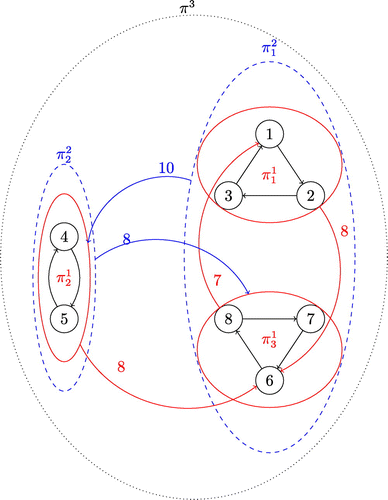
Let the set of indices be $L=\{1,2,\dots ,8\}$, and consider the matrix corresponding to the values of $\tilde{V}(K_i,K_j)$, for $i,j\in L$

$$\left(\begin{array}{cccccccc}0& 2& 4& 6& 7& 6& 12& 8\\ 6& 0& 1& 8& 9& 11& 13& 15\\ 5& 7& 0& 10& 11& 8& 9& 11\\ 5& 10& 20& 0& 3& 4& 8& 9\\ 10& 11& 12& 7& 0& 18& 16& 21\\ 7& 11& 13& 9& 11& 0& 8& 6\\ 8& 9& 14& 8& 13& 4& 0& 10\\ 15& 12& 9& 7& 10& 11& 5& 0\end{array}\right)$$

Set $L_0=L$. Using the definition above, we find three 1-cycles, ${\pi }_1^1=\{1,2,3\}$, characterized by the edges $1\to 2,\hspace{0.17em}2\to 3$, and $3\to 1,\hspace{0.17em}{\pi }_2^1=\{4,5\}$, characterized by the edges $4\to 5$, and $5\to 4$, and finally, ${\pi }_3^1=\{6,7,8\}$, characterized by the edges $6\to 8,\hspace{0.17em}8\to 7$ and $7\to 6$. Thus $L_1=\{{\pi }_1^1,{\pi }_2^1,{\pi }_3^1\}$.

Now, in order to find the 2-cycles, we use again the construction above. Straightforward computations give $\widehat{V}({\pi }_1^1)=5,\hspace{0.17em}\tilde{V}({\pi }_1^1,{\pi }_2^1)=9,\hspace{0.17em}\tilde{V}({\pi }_1^1,{\pi }_3^1)=8$. Thus, we deduce that ${\pi }_1^1\to {\pi }_1^3$. Moreover, we obtain $\widehat{V}({\pi }_3^1)=6,\hspace{0.17em}\tilde{V}({\pi }_3^1,{\pi }_1^1)=7,\hspace{0.17em}\tilde{V}({\pi }_3^1,{\pi }_2^1)=8$, and thus, ${\pi }_3^1\to {\pi }_1^1$. Finally, we find $\widehat{V}({\pi }_2^1)=7,\hspace{0.17em}\tilde{V}({\pi }_2^1,{\pi }_1^1)=9,\hspace{0.17em}\tilde{V}({\pi }_2^1,{\pi }_3^1)=8$, from which we deduce that ${\pi }_2^1\to {\pi }_3^1$. Hence, we have $L_2=\left\{\right\{{\pi }_1^1,{\pi }_3^1\},\{{\pi }_2^1\left\}\right\}$, which represents the collection of 2-cycles. Denote by ${\pi }_1^2=\{{\pi }_1^1,{\pi }_3^1\},\hspace{0.17em}{\pi }_2^2=\left\{{\pi }_2^1\right\}$ the two elements of L₂. Now, in order to identify the set of 3-cycles, we find again by simple calculations of the following quantities $\widehat{V}({\pi }_1^2)=8$, and $\tilde{V}({\pi }_1^2,{\pi }_2^2)=10$. Moreover, $\widehat{V}({\pi }_2^2)=7$ and $\tilde{V}({\pi }_2^2,{\pi }_1^2)=8$. Therefore, ${\pi }_1^2\to {\pi }_2^2$ and ${\pi }_2^2\to {\pi }_1^2$, which gives us the unique 3-cycle ${\pi }^3=\{{\pi }_1^2,{\pi }_2^2\}$, the only element of L₃. Now, we stop, because L₃ is a singleton. See Figure 2 for an illustration.

The next result gives an estimate of the mean exit time from a cycle.

Lemma 16.

Let π^k be a k-cycle, and let $i\in {\pi }^k$. Moreover, denote by $W=L\mathrm{\setminus }{\pi }^k$ the set of compacts not contained in π^k. Then, given $\epsilon >0$, there exist $\delta >0$ and $N_0\ge 1$ such that for any $r_1\le \delta ,\hspace{0.17em}\nu \in {\gamma }_i$ and $N\ge N_0$, we have

$$\exp \{N(\tilde{V}({\pi }^k)-\epsilon )\}\le {\mathbb{E}}_{\nu }[{\widehat{\tau }}_W]\le \exp \{N(\tilde{V}({\pi }^k)+\epsilon )\}.$$

Proof.

We have, from Hwang and Sheu (1990, lemma A3) and Hwang and Sheu (1990, corollary A4), that $I_i(W)=\tilde{V}({\pi }^k)$. Using this together with Lemma 14 leads to the result. □

The next result gives an estimate of the probability of going from one k-cycle to another without passing by any other element of L^k.

Lemma 17.

Let ${\pi }_1^k,\hspace{0.17em}{\pi }_2^k$ be two distinct k-cycles, and let $i\in {\pi }_1^k$. Moreover, denote $W=L\mathrm{\setminus }{\pi }_1^k$. Then, given $\epsilon >0$, there exist $\rho >0$ and $N_0\ge 1$ such that, for all $r_1\le \rho ,\hspace{0.17em}\nu \in {\gamma }_i$, and $N\ge N_0$, we have

$$\exp \{-N(\tilde{V}({\pi }_1^k,{\pi }_2^k)-\tilde{V}({\pi }_1^k)+\epsilon )\}\le P_{\nu }({\mu }^N({\widehat{\tau }}_W)\in {\gamma }_{{\pi }_2^k})\le \exp \{-N(\tilde{V}({\pi }_1^k,{\pi }_2^k)-\tilde{V}({\pi }_1^k)-\epsilon )\}.$$

Proof.

From Lemma 15 we have, for each $j\in {\pi }_2^k$ and large enough N,

$$\exp \{-N(I_{i,j}(W)+\epsilon )\}\le P_{\nu }({\mu }^N({\widehat{\tau }}_W)\in {\gamma }_j)\le \exp \{-N(I_{i,j}(W)-\epsilon )\}.$$

Therefore, summing over the disjoint compacts K_i we obtain

$${\displaystyle \sum _{j\in {\pi }_2^k}\exp }\{-N(I_{i,j}(W)+\epsilon )\}\le P_{\nu }({\mu }^N({\widehat{\tau }}_W)\in {\gamma }_{{\pi }_2^k})\le {\displaystyle \sum _{j\in {\pi }_2^k}\exp }\{-N(I_{i,j}(W)-\epsilon )\}.$$

From the sums above, we select the term decreasing more slowly than the remaining ones, which gives us

$$\exp \{-N(\min \{I_{i,j}(W):j\in {\pi }_2^k\}+\epsilon )\}\le P_{\nu }({\mu }^N({\widehat{\tau }}_W)\in {\gamma }_{{\pi }_2^k})\le \exp \{-N(\min \{I_{i,j}(W):j\in {\pi }_2^k\}-\epsilon )\}.$$

Finally, from Hwang and Sheu (1990, lemma A5), we have that $\min \{I_{ij}(W):j\in {\pi }_2^k\}=\tilde{V}({\pi }_1^k,{\pi }_2^k)-\tilde{V}({\pi }_1^k)$, which leads to the stated result. □

5.2. Convergence to the Invariant Measure

As aforementioned, there exists, under Assumption 1, a unique invariant measure ${\wp }^N$ for the empirical vector process μ^N. Thus, the distribution of μ^N converges, as time $t\to \infty$, toward ${\wp }^N$. However, one might investigate the corresponding rate of convergence. Therefore, using the results from the previous section, we show that, when the time is of order $\exp \{(\mathrm{\Lambda }+\delta )N\}$, with $\delta >0$ and Λ a suitable constant detailed above, the empirical measure is very close to its invariant measure ${\wp }^N$. Interestingly, despite the heterogeneity introduced by the block structure, a similar constant appears in the case of small-noise diffusion processes (Hwang and Sheu 1990, lemma 1.3) and in the case of homogeneous mean-field systems with jumps in Yasodharan and Sundaresan (2019, lemma 3.6). Before stating our main result, let us introduce further notations and intermediate results.

Let $i_0\in L$ be such that $\min \{\tilde{V}(g):g\in G(i_0)\}=\min \{\tilde{V}(g):g\in G(i),i\in L\}$. Moreover, define

Let $P_T(\nu ,·)=P_{\nu }({\mu }^N(T)\in ·)$ denote the transition probability kernel associated with the empirical process μ^N. The next result gives a lower bound for the transition probability $P_T(\nu ,K_{i_0})$ of reaching a small neighborhood of $K_{i_0}$ when T is of order $\exp \{N(\mathrm{\Lambda }-{\delta }_0)\}$ for some ${\delta }_0>0$.

Theorem 6.

Given $\epsilon >0$, there exist ${\delta }_0>0$, r > 0, and $N_0\ge 1$ such that, for all $r_1\le r$, $N\ge N_0$, and $\nu \in {({\mathcal{M}}_1(\mathcal{Z}))}^{2r}$, we have

$$P_{T_0}(\nu ,{\gamma }_{i_0})\ge \exp \{-N\epsilon \},$$

where $T_0=\exp \{N(\mathrm{\Lambda }-{\delta }_0)\}$. Furthermore, there exist ${\nu }_0\in {({\mathcal{M}}_1(\mathcal{Z}))}^{2r}$ and $\beta >0$ such that, for all $N\ge N_0$ and $\nu \in {[{\nu }_0]}_{r_1}$,

$$P_{T_0}(\nu ,{\gamma }_{i_0})\le \exp \{-N\beta \}.$$

Proof.

Replacing the space ${\mathcal{M}}_1(\mathcal{Z})$ by the product space ${({\mathcal{M}}_1(\mathcal{Z}))}^{2r}$ together with the corresponding metrics, the proof given in Yasodharan and Sundaresan (2019, theorem 3.21) adapted from Hwang and Sheu (1990, theorem 2.3, part I) holds verbatim. □

Corollary 2.

Under the conditions of Theorem 6, for all $\nu \in {({\mathcal{M}}_1(\mathcal{Z}))}^{2r},\hspace{0.17em}\xi \in {\gamma }_{i_0}$, and N sufficiently large, we have

$$P_{T_0}(\nu ,\xi )\ge \exp \{-2N\epsilon \}.$$

Proof.

The proof follows verbatim the proof given in Yasodharan and Sundaresan (2019, corollary 3.22). □

We state now the main result of this section, which gives the time scale at which the empirical vector converges toward its invariant measure.

Theorem 7.

There exists a constant $\mathrm{\Lambda }\ge 0$ such that, for any $\delta >0$, there exist $\epsilon >0$ and $N_0\ge 1$ such that, for all $\nu \in {({\mathcal{M}}_1(\mathcal{Z}))}^{2r}$ and $N\ge N_0$,

$$\left|{\mathbb{E}}_{\nu }\left[f({\mu }^N(T))\right]-{\displaystyle \int f}d{\wp }^N\right|\le \Vert f{\Vert }_{\infty }\exp \{-\exp (N\epsilon )\},$$

where $T=\exp \{N(\mathrm{\Lambda }+\delta )\}$ and f is any bounded and measurable function on ${({\mathcal{M}}_1(\mathcal{Z}))}^{2r}$.

Proof.

Let $\epsilon >0$, and let T₀, δ₀, r, r₁, and $N_0\ge 1$ be as in the statement of Theorem 6. By Corollary 2 we have that, for any $\nu \in {({\mathcal{M}}_1(\mathcal{Z}))}^{2r}$ and $\xi \in {[K_{i_0}]}_{r_1}$,

$$P_{T_0}(\nu ,\xi )\ge \exp \{-2N\epsilon \}.$$(5.2)

Moreover, by the Markov property and using Corollaries 2 and 1, we have that, for any $\nu \in {({\mathcal{M}}_1(\mathcal{Z}))}^{2r},\hspace{0.17em}\xi \notin {[K_{i_0}]}_{r_1}$, and some fixed t,

$$\begin{array}{ll}{P}_{T_0}(\nu ,\xi )\hfill & \ge {\displaystyle \sum _{{\nu }^{\prime }\in [K_{i_0}]}{P}_{T_0-t}}(\nu ,{\nu }^{\prime })P_t({\nu }^{\prime },\xi )\hfill \\ \hfill & \ge \exp \{-2N\epsilon \}\underset{{\nu }^{\prime }\in [K_{i_0}]}{\inf }{P}_t({\nu }^{\prime },\xi )\hfill \\ \hfill & \ge \exp \{-2N\epsilon \}\exp \{-N\underset{{\nu }^{\prime }\in [K_{i_0}]}{\sup }{S}_t(\xi |{\nu }^{\prime })\},\hfill \end{array}$$(5.3)

for sufficiently large N. Notice that, thanks to (5.2) and because $S_T(\xi ,\nu )$ is bounded for all $\nu ,\xi \in {({\mathcal{M}}_1(\mathcal{Z}))}^{2r}$, one can find a positive function $U(\xi )$ such that $U(\xi )=0$ for $\xi \in {[K_{i_0}]}_{r_1}$, and $U(\xi )\ge {\sup }_{{\nu }^{\prime }\in [K_{i_0}]}{S}_t(\xi |{\nu }^{\prime })$ for $\xi \notin {[K_{i_0}]}_{r_1}$.

Define ${\pi }_N(\xi )=c_N\exp \{-NU(\xi )\}$ such that $U(\xi )=0$ for $\xi \in {[K_{i_0}]}_{r_1}$, and

$$P_{T_0}(\nu ,\xi )\ge c_N\exp \{-NU(\xi )\}$$

for all $\nu \in {({\mathcal{M}}_1(\mathcal{Z}))}^{2r},\hspace{0.17em}\xi \notin [K_{i_0}]$, and sufficiently large N, where c_N is a constant chosen such that π_N is a probability measure on the product space ${({\mathcal{M}}_1(\mathcal{Z}))}^{2r}$. Moreover, set $Q_{T_0}(\nu ,·)=P_{T_0}(\nu ,·)/{\pi }_N(·)$. Hence, by (5.2), $Q_{T_0}(\nu ,\xi )\ge 1$ for any $\nu ,\xi \in {({\mathcal{M}}_1(\mathcal{Z}))}^{2r}$. Let f be a bounded measurable function on ${({\mathcal{M}}_1(\mathcal{Z}))}^{2r}$. Therefore, for any ${\nu }_1,{\nu }_2\in {({\mathcal{M}}_1(\mathcal{Z}))}^{2r}$ and sufficiently large N, we have

$$\begin{array}{ll}{\mathbb{E}}_{{\nu }_1}(f({\mu }^N(T_0)))-{\mathbb{E}}_{{\nu }_2}(f({\mu }^N(T_0)))\hfill & ={\displaystyle {\int }_{{({\mathcal{M}}_1(\mathcal{Z}))}^{2r}}f}(\xi )P_{T_0}({\nu }_1,d\xi )-{\displaystyle {\int }_{{({\mathcal{M}}_1(\mathcal{Z}))}^{2r}}f}(\xi )P_{T_0}({\nu }_2,d\xi )\hfill \\ \hfill & ={\displaystyle {\int }_{{({\mathcal{M}}_1(\mathcal{Z}))}^{2r}}f}(\xi )Q_{T_0}({\nu }_1,d\xi ){\pi }_N(d\xi )-{\displaystyle {\int }_{{({\mathcal{M}}_1(\mathcal{Z}))}^{2r}}f}(\xi )Q_{T_0}({\nu }_2,d\xi ){\pi }_N(d\xi )\hfill \\ \hfill & ={\displaystyle {\int }_{{({\mathcal{M}}_1(\mathcal{Z}))}^{2r}}f}(\xi )(Q_{T_0}({\nu }_1,d\xi )-\exp \{-2N\epsilon \}){\pi }_N(d\xi )\hfill \\ \hfill & -{\displaystyle {\int }_{{({\mathcal{M}}_1(\mathcal{Z}))}^{2r}}f}(\xi )(Q_{T_0}({\nu }_2,d\xi )-\exp \{-2N\epsilon \}){\pi }_N(d\xi )\hfill \\ \hfill & \le \underset{\xi \in {({\mathcal{M}}_1(\mathcal{Z}))}^{2r}}{\sup }f(\xi )(1-\exp \{-2N\epsilon \})\hfill \\ \hfill & -\underset{\xi \in {({\mathcal{M}}_1(\mathcal{Z}))}^{2r}}{\inf }f(\xi )(1-\exp \{-2N\epsilon \})\hfill \\ \hfill & =(1-\exp \{-2N\epsilon \})|\underset{\xi }{\sup }f(\xi )-\underset{\xi }{\inf }f(\xi )|.\hfill \end{array}$$(5.4)

Thence we find,

$$\begin{array}{l}\underset{{\nu }_1,{\nu }_2}{\sup }\left|{\mathbb{E}}_{{\nu }_1}(f({\mu }^N(T_0)))-{\mathbb{E}}_{{\nu }_2}(f({\mu }^N(T_0)))\right|\le (1-\exp \{-2N\epsilon \})\Vert f{\Vert }_{\infty }.\hfill \end{array}$$(5.5)

Hence, by repeating the previous steps k times using the Chapman-Kolmogorov property given that μ^N is Markov, we find

$$\begin{array}{l}\underset{{\nu }_1,{\nu }_2}{\sup }\left|{\mathbb{E}}_{{\nu }_1}(f({\mu }^N(k{T}_0)))-{\mathbb{E}}_{{\nu }_2}(f({\mu }^N(k{T}_0)))\right|\le {(1-\exp \{-2N\epsilon \})}^k\Vert f{\Vert }_{\infty },\hfill \end{array}$$(5.6)

from which we deduce that

$$\begin{array}{l}\underset{\nu }{\sup }\left|{\mathbb{E}}_{\nu }(f({\mu }^N(k{T}_0)))-〈{\wp }^N,f〉\right|\le {(1-\exp \{-2N\epsilon \})}^k\Vert f{\Vert }_{\infty }.\hfill \end{array}$$(5.7)

Choose $k=\exp \{N({\delta }_0+\delta )\}$. Thus, $k{T}_0=\exp \{N(\delta +\mathrm{\Lambda })\}$. Moreover, using the property ${\left(1+\frac{x}{n}\right)}^n\to \exp \left\{x\right\}$ as $n\to \infty$, one obtains for large k

$$\begin{array}{l}\underset{\nu }{\sup }\left|{\mathbb{E}}_{\nu }(f({\mu }^N(k{T}_0)))-〈{\wp }^N,f〉\right|\le \exp \{-\exp \{N(-2\epsilon +{\delta }_0+\delta )\left\}\right\}\Vert f{\Vert }_{\infty }.\hfill \end{array}$$(5.8)

Choosing ε small enough such that ${\epsilon }^{\prime }=-2\epsilon +{\delta }_0+\delta >0$, one finally obtains

$$\begin{array}{l}\underset{\nu }{\sup }\left|{\mathbb{E}}_{\nu }(f({\mu }^N(T)))-〈{\wp }^N,f〉\right|\le \exp \{-\exp \{N{\epsilon }^{\prime }\left\}\right\}\Vert f{\Vert }_{\infty },\hfill \end{array}$$(5.9)

for large enough N, with $T=\exp \{N(\delta +\mathrm{\Lambda })\}$. The theorem is proven. □

6. Conclusion and Discussion

We have addressed in this paper the large-time behavior of the empirical measure vector associated with a family of finite-state mean-field models with multiclasses. In particular, we have established the large deviations principle for the invariant measure when the McKean-Vlasov limiting system has a unique asymptotically stable equilibrium and when there are multiple ω-limits sets. Also, we established various metastability phenomena estimates together with the speed of convergence of the empirical measure vector to its invariant measure. These results are of interest for various real-world applications ranging from engineering systems to the spread of infectious diseases. In particular, the multispecies setting represented by the block graph structure can be used as a model for various phenomena.

Many interesting questions remain nevertheless open and are worthwhile to explore. For instance, for the family of block graphs analyzed in the current paper, the degree of each node is O(N). An interesting extension is to consider other scaling regimes for the degree of the nodes. For example, the number of neighbors of the peripheral nodes could grow as $O(\sqrt{N})$. Even though it is sublinear in N, there could be a strong interaction. It would be interesting to study the large-time behavior of the vector empirical measure process in such cases.

The asymptotic analysis conducted in the current paper is on the vector of empirical measures. However, one might be interested to study the large deviation of the global empirical measure. Given the heterogeneity of the particles composing the global empirical measure, the latter is not a Markov process. Yet from the large deviations of the vector of empirical measures, one can use the contraction principle to deduce the large deviations principle for the sequence of global empirical measures. The question then is to understand the rate function. Another interesting question is to find criteria for the uniqueness of stationary distribution of the global empirical measure.

A natural extension of the current work is to consider the case of countable state spaces. Notice that if one replaces the finite space $\mathcal{Z}$ by a countable state space $E=\{0,1,2,\dots \}$, the corresponding set ${\mathcal{M}}_1(E)$ of probability measures over E is no longer compact or finite-dimensional. Therefore, one has to impose stronger conditions on the rate functions to study the asymptotics of the system. For instance, the large deviations principle of the empirical measures has been established in Feng (1994) and Léonard (1995a) under different assumptions on the Levy kernels governing the jumps. However, the large deviations principle for the family of invariant measures is not available in the general countable state-space context and thus remains an open problem. In a recent contribution, Yasodharan and Sundaresan (2021), sufficient conditions have been established for a class of interacting particle systems on countable state space under which the sequence of invariant measures satisfies the large derivation principle with a rate function governed by the Freidlin-Wentzell quasipotential. Nonetheless, the proofs in Yasodharan and Sundaresan (2021) hold only under specific conditions on the transition graph and the forward transition rates. Also, the results in Yasodharan and Sundaresan (2021) are restricted to the case where the limiting McKean-Vlasov system has a unique globally asymptotically stable equilibrium and do not hold when there are multiple ω-limit sets. Thus, the latter case remains open to exploration. In particular, the Freidlin-Wentzell approach for studying large deviations of the invariant measures used in the current paper is not directly applicable in the case of countable state space because it requires the uniform large deviations principle over open subsets of ${\mathcal{M}}_1(E)$, which is not available. Consequently, one cannot use this approach to study the related exit problems and metastability phenomena. It is then a challenging open question. Of course, these challenges are heightened in the multiclasses context considered in the current paper due to the technicalities arising from the product space setting.

References

- (2008) A class of mean field interaction models for computer and communication systems. Perform. Eval. 65(11–12):823–838.Google Scholar
- (1999) Convergence of Probability Measures (John Wiley & Sons, New York).Google Scholar
- (2011) Small noise asymptotics for invariant densities for a class of diffusions: A control theoretic view (with erratum). Preprint, submitted, https://arxiv.org/abs/1107.2277.Google Scholar
- (2012) Asymptotics of the invariant measure in mean field models with jumps. Stoch. Syst. 2(2):322–380.Link, Google Scholar
- (2016) Perturbative calculation of quasi-potential in non-equilibrium diffusions: A mean-field example. J. Stat. Phys. 163:1157–1210.Google Scholar
- (2019) Partial mean field limits in heterogeneous networks. Stochastic Process. Appl. 129:4998–5036.Google Scholar
- (2014) Macroscopic Limit of a bipartite Curie-Weiss model: A dynamical approach. J. Stat. Phys. 157:1309–1319.Google Scholar
- (2016) Rhythmic behavior in a two-population mean-field Ising model. Phys. Rev. E. 94:042139.Google Scholar
- (1990) On the long term behavior of some finite particle systems. Probab. Theory Related Fields 85:195–237.Google Scholar
- (1987) Large deviations from the McKean-Vlasov limit for weakly interacting diffusions. Stochastics 20(4):247–308.Google Scholar
- (1989) Large deviations, free energy functional and quasipotential for a mean field model of interacting diffusions. Mem. Amer. Math. Soc. 78(398).Google Scholar
- (1993) Hierarchical models of interacting diffusions: Multiple time scale phenomena, phase transition, and pattern of cluster-formation. Probab. Theory Related Fields 96:435–473.Google Scholar
- (1999) Hierarchically interacting Fleming-Viot processes with selection and mutation: Multiple space time scale analysis and quasi-equilibria. Electron. J. Probab. 4:1–81.Google Scholar
- (1995) Equilibria and quasi-equilibria for infinite collections of interacting Fleming-Viot processes. Trans. Amer. Math. Soc. 347(7):2277–2360.Google Scholar
- (2020) Propagation of chaos and large deviations in mean-field models with jumps on block-structured networks. Preprint, submitted December 4, https://arxiv.org/abs/2012.02870.Google Scholar
- (2010) Large Deviations Techniques and Applications, 2nd ed. (Springer, New York).Google Scholar
- (2013) Longtime Behavior for Mutually Catalytic Branching with Negative Correlations, vol. 38 (Springer Proceedings in Mathematics & Statistics, Boston).Google Scholar
- (2006) Large Deviations for Stochastic Processes (Mathematical Surveys and Monographs, American Mathematical Society).Google Scholar
- (1994) Large deviations for empirical process of mean-field interacting particle system with unbounded jumps. Ann. Probab. 22(4):2122–2151.Google Scholar
- (2012) Random Perturbations of Dynamical Systems, 3rd ed. (Springer, Berlin-Heidelberg).Google Scholar
- (2008) Chaoticity for multiclass systems and exchangeability within classes. J. Appl. Probab. 45:1196–1203.Google Scholar
- (2007) Phase transitions for the long-time behavior of interacting diffusions. Ann. Probab. 35(4):1250–1306.Google Scholar
- (1990) Large-time behavior of perturbed diffusion Markov processes with applications to the second eigenvalue problem for Fokker-Planck operators and simulated annealing. Acta Appl. Math. 19:253–295.Google Scholar
- (2020) Fluctuation results for general block spin Ising models. J. Stat. Phys. 178(1):1175–1200.Google Scholar
- (2015) Multiple Time Scale Dynamics (Springer International Publishing, Switzerland).Google Scholar
- (1995a) Large deviations for long range interacting particle systems with jumps. Annales de l’I.H.P. Probabilités et Statistiques, Tome 31 31(2):289–323.Google Scholar
- (1995b) On large deviations for particle systems associated with spatially homogeneous Boltzmann type equations. Probab. Theory Related Fields 101:1–44.Google Scholar
- (2020) Two-community noisy Kuramoto model. Nonlinearity 33(4):1847–1880.Google Scholar
- (2020) On mean field systems with multi-classes. Discrete Contin. Dyn. Syst. 40(2):683–707.Google Scholar
- (2017) Potential landscape of high dimensional nonlinear stochastic dynamics with large noise. Sci. Rep. 7(15762):1157–1210.Google Scholar
- (2019) Large time behaviour and the second eigenvalue problem for finite state mean-field interacting particle systems. Preprint, submitted September 9, https://arxiv.org/abs/1909.03805.Google Scholar
- (2021) A sufficient condition for the quasipotential to be the rate function of the invariant measure of countable-state mean-field interacting particle systems. Preprint, submitted October 25, https://arxiv.org/abs/2110.12640.Google Scholar
- (2012) Quasi-potential landscape in complex multi-stable systems. R. Soc. Interface 9:3539–3553.Google Scholar