Accuracy of the Graphon Mean Field Approximation for Interacting Particle Systems
Abstract
We consider a system of N particles whose interactions are characterized by a (weighted) graph . Each particle is a node of the graph with an internal state. This state changes according to Markovian dynamics that depend on the states of neighboring particles. We study the limiting properties of the state dynamics, focusing on the dense graph regime, in which the average degree of a node grows linearly with N. We show that, when converges to a piecewise Lipschitz graphon G, the behavior of the system converges to a deterministic limit, the graphon mean field approximation. We obtain convergence rates depending on the system size N and cut-norm distance between and G. We apply these results for two subcases: when is a discretization of the graph G with individually weighted edges; when is a random graph obtained by sampling edges with probabilities obtained from G. In the case of weighted interactions, we obtain a bound of order . In the random graph case, the error is of order with high probability. We illustrate the applicability of our results and the numerical efficiency of the approximation through two examples: a graph-based load-balancing model and a heterogeneous bike-sharing system.
Funding: This work was supported by the ANR (Agence National de la Recherche), via the project REFINO (ANR-19-CE23-0015).
Supplemental Material: The online appendix is available at https://doi.org/10.1287/stsy.2024.0070.
1. Introduction
Mean field approximations are ubiquitously used in the study of large-scale stochastic systems. Its mathematical foundations date back to the 1960s and 1970s with the seminal papers of Kurtz (1970, 1971), McKean (1967), and Norman (1972). Whereas originating from statistical physics, the mean field methodology has found application in many areas, such as communication networks Le Boudec et al. (2007), load balancing Mitzenmacher (2001), and the study of epidemics Roy et al. (2023). The fundamental idea of the mean field method is to represent the particle process by a Markovian state descriptor based on averaged quantities of the system. A quantity commonly used in this context is state occupancy processes, for example, the averaged load of stations for a bike sharing system (Fricker and Gast 2016) or the fraction of servers having at least a certain queue length for load-balancing systems (Mitzenmacher 2001). To apply the classic mean field method, it is crucial that the particles of the system are homogeneous and, therefore, interchangeable, ensuring the Markov property for the mentioned aggregate quantities. Its applicability to real-world scenarios is often hindered by the intrinsically heterogeneous behavior of realistic models as heterogeneity breaks the quintessential exchangeability assumption. Therefore, it is necessary to keep track of the evolution of the whole set of particles in the system, which makes the application of classic mean field methods complicated if not infeasible.
To overcome these difficulties, mean field models that use graphons as a description of diversity of individuals and the variation of their interaction have been proposed (Budhiraja et al. 2019, Vizuete et al. 2020, Bayraktar et al. 2023, Keliger 2023, Bet et al. 2024). One example for when this approach finds widespread application are epidemic models for which graphons characterize the epidemic propagation (Decreusefond et al. 2012, Aurell et al. 2022, Delmas et al. 2023, Roy et al. 2023). For many settings, results show that deterministic graphon-based models are limiting processes for sequences of graph-based interacting and densely connected particle systems. Whereas the use of the graphon mean field model is well-justified, the bias and convergence speed in its application can vary immensely depending on the convergence properties of the considered graph sequence. Surprisingly, the literature concerning the issue of convergence rates and accuracy is relatively sparse. This paper contributes to filling this gap as we derive generic bounds on the bias for the graphon approximation for finite-sized and densely connected interacting particle systems.
1.1. Contributions
We provide bias bounds for the graphon mean field approximation for finite-sized systems consisting of interacting particles for which the graph models the connection of the population. Our results show that it is possible to derive bias bounds that largely depend on the convergence properties of the graph sequence and of its limiting graphon G. To be more precise, we start from a stochastic interacting particle model of finite size N, where each individual k is characterized by a time-varying state . The connection of the particle to the population is given by the edges of a graph . Based on this description, we construct a (deterministic) integro-differential equation based on the graphon G and show that it has a unique solution that we call the graphon mean field approximation. This differential equation is constructed such that, for fixed N, approximates the probability of particle to be in state s at time t. Denoting this probability, our main result shows that
To show the extent of the result, we consider two specific graph-sampling strategies for . In the first case (which we denote deterministic sampling), is the discretization of the limiting graphon G with being the strength of interaction between two particles. We consider this case as it illustrates how our result can be used to model a system composed of heterogeneous particles. In the second case (which we call stochastic sampling), is a random graph generated from G, where an edge is present between two nodes k and with probability . The second case corresponds to a generalization of Erdős–Rényi graph and stochastic block models to possibly nonuniform probabilities.
Imposing some mild assumptions, such as a piecewise Lipschitz condition on the graphon G or symmetry of G, in the case of stochastic sampling, we can bound the distance between the graph and the graphon G by
1.2. Organization
The paper is organized as follows. In Section 2, we introduce the heterogeneous particle model. Section 3 defines graphon, related sampling methods, and related preliminary results. Our definition of the approximation, the main results, and the proofs are displayed in Section 4. In Section 5, we present the two numerical examples. Finally, we conclude in Section 7 in which we discuss limitations and future work.
1.3. Related Work
1.3.1. Dynamical Systems on Random Graphs.
In recent years, there has been growing interest in the behavior of interacting particles that are interconnected by an underlying graph topology (e.g., Abbe 2018, Bhamidi et al. 2019, Bayraktar and Wu 2021, Bet et al. 2024, and previously mentioned references). For a general introduction to the topic of random graph networks and limiting graphon functions for dense graphs, we refer to the works Van Der Hofstad (2017) and Lovász (2012). The majority of papers focus on dense graphs, having edges of order such as Erdős–Rényi type graphs or graphs generated by stochastic block models. Additional related work can be found in the game-theoretic setting for graphon mean field games; see, for example, Caines and Huang (2021) and Aurell et al. (2022). In the not-so-dense setting, available results are more limited with some newer references being Bayraktar et al. (2023) and Delmas et al. (2023). In the case of sparse graphs, such as d-regular graphs or random geometric graphs, the typical mean field methods break down as they fail to capture the importance of the spatial graph structure and its implications on the local dynamics of particles. Some recent works in this setting include Ganguly and Ramanan (2024), Ramanan (2022), and Ganguly (2022).
1.3.2. Load Balancing on Graphs.
Our load-balancing example is inspired by the recent works of Rutten and Mukherjee (2023), Zhao and Mukherjee (2024), Zhao et al. (2024), and Budhiraja et al. (2019). Here, the authors study a variety of load-balancing systems with dynamics based on compatibility or locality constraints, and these give rise to intricate connectivity between dispatchers and servers. Whereas not directly transferable into the framework of this paper, the authors similarly deal with graph-based systems and limit approximations that are strongly related to the ones our framework suggests. Note that the techniques developed in these papers are very model-specific and allow for transitions to depend on the states of multiple queues, whereas our approach aims at deriving results for a more general framework for transition rates with the restriction to the case of pair interactions.
1.3.3. Generator and Stein’s Method.
For our proofs, we adapt techniques used in Gast and Van Houdt (2017), Allmeier and Gast (2022), and Gast (2017), which, in turn, rely on the use of Stein’s (1986) method. The method is used to estimate and bound the distance between two random variables through their respective generators. Since the publication of works Braverman et al. (2017) and Braverman and Dai (2017), Stein’s (1986) method has seen an increase in the stochastic network community and is an actively evolving area.
2. Heterogeneous Network Particle System
2.1. The Interaction Model
We consider particle systems with interacting particles. Connections between particles are characterized by a (possibly weighted) adjacency matrix , with indicating the connection strength between particle k and l. Each of the particles has a finite state space , where the state of the kth object at time is denoted by . As we see later, can correspond to a random graph for which indicates the presence or absence of an undirected edge between the particles k and l or can be an arbitrary weight matrix; see Section 3. The state of the whole system is denoted by . We assume that the process is a continuous time Markov chain with the dynamics of the system described as in the following. Each particle changes its state from to in one of two ways:
(Unilateral) The change of state occurs at rate independently of the other particles.
(Pairwise) The change of state is triggered by another particle that is in state . This occurs at rate .
Note that the rate functions are assumed to be heterogeneous; that is, they can depend on the items k and l. The rates have a factor as each particle can potentially interact with all remaining particles. Hence, our condition implies that the total rate of transitions of the particle system is of order and that the transition rates for all particles are of the same order. We show in Example 5.1 that our result can also be used if the scaling factor depends not on the system size N but on the average degrees. We further want to point out that we restrict our framework to the interaction of two particles, and these can be utilized to model many relevant interacting particle systems on graphs such as, for example, epidemic spreading, power-of-two-choices load-balancing, or bike-sharing systems. It is nonetheless possible to use the same underlying approach to extend the framework and results to interactions between more than two particles by modeling, for instance, the interaction between more than two particles as hypergraphs. This, however, comes at the cost of increasingly cumbersome notations and limited added theoretical insight.
2.2. The Binary State Representation
In order to ease computations and definitions, we use a binary representation of the state based on indicator functions. We denote the new representation by , where
The space of attainable states is denoted by .
Whereas this representation is less compact than the original, it allows for an easier definition of transition rates as well as the definition of the mean field approximation. Denote by a matrix of size whose component is equal to one, all other entries being zero. For each , and , jumps to at rate
In the above equation, the first term of the rate corresponds to the unilateral transition of the particle changing its state from to as this transition occurs at intensity if particle k is in state (i.e., ). The second term describes the pairwise transitions leading to the state change of particle k from to . Similar to the unilateral one, the transition can only happen if particle k is in state , represented in the rate by the prefactor . The remaining factor corresponds to the interaction with other particles, expressed by the weighted sum over all other particles and their states. The intensity of the transition is scaled by , and the connectivity of the particles is given by the connectivity matrix .
2.3. Drift of the System of Size N
By using the state representation , we define what we call the drift of the system of N particles as the expected change for in state . It is equal to the sum of all possible transitions of the changes induced by this transition times the rate at which the transition occurs. We denote this quantity as . By using Equation (2), it is equal to
The quantity is a vector-valued function of . By reorganizing the above sum, —its component—is equal to
In the following, it is convenient to replace the above sum by matrix multiplications. To do so, let us denote by the vector . The above equation can be written as
2.4. Representation of , , and as Functions from
To study the limit as N goes to infinity, it is convenient to view the functions not as a vector with N components but as a step function , where for any state , we set
By abuse of notation, we do not introduce separate notations for the discrete and continuous variables but make the distinction by reserving the subscript letters for the discrete case and for the continuous variable.
Similarly, we also write for and , , and . By using this notation, the sum of —for instance in (3)—can be replaced by an integral, that is, for .
2.5. Notations
Throughout the paper, matrices and vectors are written in bold letters, that is, , and regular letters are used to denote scalars such as . The indices are reserved for the states; k, l, ... are reserved for particles; and u, v are reserved for values in the unit interval. When we write that a quantity h is of order or equivalently, this means that there exists a constant C such that . Such a constant C might depend on the model considered (the graphon or the rate functions). Most of our results are expressed in terms of norm (see the definition in Section 3.3). The space refers to the quotient space of the square Lebesgue integrable functions. Throughout, we deal with vectors of functions, that is, . For two vectors g, f we denote the scalar product by and the induced norm . For a function denote by Gf the function defined as . We denote the norm-operator of G as
3. Limiting Graph and Graphon
In this section, we specify the properties that the interaction graph needs to satisfy as N goes to infinity. To do so, we introduce the notion of graphon and define the associated cut-norm. We also introduce two sampling methods that can be used to generate a graph with N nodes from a graphon. This section only reviews the material that is necessary for our results, and we refer to the famous book Lovász (2012) for a detailed introduction to graphons.
3.1. Graphons
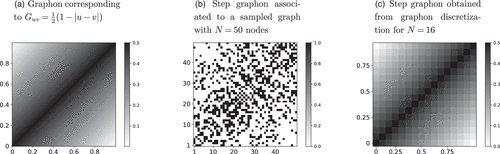
In this paper, what we call a graphon is a measurable function2 . The notion of graphon can be viewed as a generalization of the notion of graph. Indeed, for any N, a weighted graph can be viewed as a piecewise constant function defined on , where the value of this function at a point is equal to whenever and . Hence, a finite graph is a graphon that has a special structure. The notion of graphon generalizes the notion of a finite graph by allowing G to be any measurable function. We provide an illustration of a graphon and of a finite graph viewed as a graphon on Figure 1.
Throughout the paper, we consider piecewise Lipschitz continuous graphons, which are defined as follows.
(
A particular case of a piecewise Lipschitz continuous graphon is the case of a step graphon, that is such that the Lipschitz constant . This implies that the function G is constant on all intervals . For instance, all finite graphs can be seen as step graphons by using the partition such that with N being the number of nodes in the graph.
3.2. Generation of a Finite Graph from a Graphon G
Based on a given graphon G, we consider two distinct sampling methods to generate a finite graph from G:
In the first case, termed deterministic sampling, is a discretization of G on uniformly sampled points, that is, for .
For the second case, termed stochastic sampling, and under the preliminary assumption that the graphon is symmetric, the values are drawn according to independent Bernoulli random variables, that is, , and for all .
In the case that the graphon is constant for all , the stochastic sampling method is equivalent to sampling an Erdős–Rényi graph. If the graphon is block-wise constant, the sampling is similar to the stochastic block model; see Van Der Hofstad (2017).
3.3. Graphon Distances and Convergence
To measure the distance between two graphs (and, in particular, to quantify how fast a finite graph converges to G), we use the operator norm as defined in Section 2.5. More precisely, for a measurable function , we denote by the norm of f. For a graphon G, we denote by the operator norm of G in , that is
The distance between two graphons (or finite graphs) G and is measured as .
To bound the distance between a piecewise Lipschitz graphon and the function associated with a randomly sampled graph, we utilize the results displayed in Avella-Medina et al. (2018). The authors show that, for a large enough (see Definition 2) number N of graph nodes, in our case particles, the distance between the graphon and the graph function can be upper bounded as follows.
(
(
Implied by Theorem 1, by setting , we see that the distance between a piecewise Lipschitz graphon and a sampled graph is with high probability of order . The meaning of “with high probability” in this context is that the right-hand side holds with probability at least .
4. Main Results
4.1. Assumptions
In Section 2, we constructed a model that depends on a scaling parameter N. We now state the assumptions that we use to state the accuracy of the graphon mean field approximation.
(A1) The state space is finite.
(A2) The graphon G is piecewise Lipschitz continuous.
(A3) There exists bounded and piecewise Lipschitz-continuous rate functions for and for and such that the rates function of the original N particle systems have the relation:
(6)
The first assumption on the finiteness of the state-space is not necessary per se but simplifies the exposition of the results. Our results can be generalized to countable state-space but at the price of extra assumptions that would clutter the readability of the paper. Imposing a finite state-space simplifies the definition of the space. To allow for nonfinite , one needs to add not just a uniform bound on the transition rates (such as ) but a bound on their norm in this infinite-dimensional space: in our proof, some bounds depend on (see, for instance, Online Lemma 7) because only provides a bound on the infinite-norm of the rate functions. When is finite, all such norms are equivalent. The second assumption is a regularity assumption that we use to obtain bounds on the rate at which a sequence of graphs converges to graphons. As shown in Lovász (2012, lemma 11.33), some regularity assumptions on G are needed to show the convergence. In practice, our bounds depend on the distance between the original graph and the graphon G. The last assumption ensures that the particle transition rates for the finite and the graphon system are equal. We point out that assumption () can be generalized by replacing the equality in (6) with bounds for the distance of and , therefore modifying the bounds of the theorem to include terms of the form .
4.2. The Graphon Mean Field Approximation
The graphon mean field approximation aims at approximating the dynamics of the original system . We define the graphon-related drift similarly to the drift of the particle system in Equation (3). For , the graphon-based drift is defined by
Based on the drift function and the initial condition , we call the graphon mean field approximation the solution of the differential equation
Let denote the deterministic drift defined in Equation (7) and the value of the solution of the graphon mean field approximation at time t with initial condition as in Equation (8). It holds that, for all t and all initial conditions , is well-defined and unique (in ) and is differentiable with respect to its initial condition. Furthermore, this derivative is Lipschitz continuous.
The proof is postponed to Section 6.1.
4.3. Accuracy of the Approximation
The following result provides a bound on the distance between the stochastic system and the graphon mean field approximation. This bound is stated as the distance between and . Recall that, by definition, is the probability for an item k to be in state s at time t. Hence, our theorem shows that the graphon mean field model is an accurate approximation of the state distribution of the particles. The statement of the theorem should be interpreted as saying that the distribution of the particles over the states for any time is approximated by the graphon mean field approximation with accuracy depending on the system size N as well as the distance between and graphon G. In particular, if converges to G (for the graphon norm), then the graphon mean field approximation is asymptotically exact.
(
The proof of Theorem 1 is postponed to Section 6.2. The constants of Equation (9) depend on the uniform bound of the rates, the time t, and the Lipschitz constants of the graphon. In the subsequent Corollaries 1 and 2, we see that, if the is generated by one of the methods illustrated in Section 3.2, precise bounds on the distance can be obtained. To illustrate our results and underline that the constants are small in practice, we provide examples in Section 5. We point out that Theorem 1 is applicable for a wide range of construction methods for . The subsequent corollaries illustrate cases of stochastic and deterministic sampling methods. We emphasize, however, that any method that allows the construction of densely connected graphs, for which bounds of are attainable, is viable. At last, we want to point out that, by using the same framework, it seems feasible to extend our results to interactions of triplets or higher order interactions. Yet, because of our generic choice of transition rates, this would be linked to increasingly heavy notations for the dynamics, only giving little more insight into the accuracy of the graphon mean field method.
A nice interpretation of Theorem 1 is in terms of total variation distance. Indeed, by definition of as an indicator function (1), we have . The total variation distance between two distributions and is equal to . Hence, by the Cauchy–Schwarz inequality, one has
The above equation shows that, on average, the law of a particle k converges to . Note that this does not mean that the law of each particle k converges to . For instance, changing all edges of a single particle only changes by a factor .
4.4. Case-Specific Bounds for
The subsequent corollaries give specific bounds for the case that was generated as described in Section 3.2. In the first case, if is obtained though discretization of G, Corollary 1 shows that the accuracy is of order . Our second Corollary 2 specifies big- convergence rates if the graph is sampled stochastically from the graphon. In this case, the accuracy is with high probability of order .
4.4.1. Case 1: Graphon Discretization.
The corollary provides a bound on the accuracy of the approximation in the case that the graph is obtained as a discretized version of G. The result gives bounds on the difference between the distributions of the particles in the stochastic system and the approximate values obtained through the graphon mean field approximation.
(
The proof is postponed to Section 6.3. The constants are as in Theorem 1. The additional constant relates to the discretization error of the deterministic sampling method. For this case, it is noteworthy that the accuracy of the approximation aligns with the results one obtains for the homogeneous setting as described in Gast (2017) and Gast and Van Houdt (2017), allowing for heterogeneous connectivity and rates among the population.
4.4.2. Case 2: Random Graph.
Our second corollary provides accuracy bounds for interacting particle systems on dense random graphs. By the definition of the graph-sampling methods, see Section 3.2, with high probability, the number of connected neighbors for each particle is of order N. This ensures that, for large enough systems that the neighborhood of each node serves as a local representation of the overall system state. This leads to the following result.
(
where with being the Lipschitz constant of the graphon G and the size of the partition as defined in (1).
In the above theorems, the constants and are a measure of heterogeneity of the nodes of the graphon. If G represents a stochastic bloc model, then and corresponds to the number of blocks. If the graphon represents a continuous popularity (as in Figure 1 or in our bike-sharing example), then . A graphon with a large or a large would represent a graph in which the nodes have a very heterogeneous behavior.
The proof of the corollary is postponed to Section 6.3.
5. Numerical Experiments
In this section, we present two examples that support the statements of our theoretical results and illustrate the applicability of the framework. For the first example, we look at a load-balancing model with communication restrictions of the servers imposed by a graph. In this example, the focus is on the stochastically sampled graph, which imposes heterogeneous rates because of the connectedness of the servers. For the dynamics of the system, we see each node as a dispatcher–server pair applying the JSQ(2) policy with respect to itself and connected servers whenever a job arrives. For the second example, we consider a heterogeneous bike-sharing system. Here, the focus lies on the heterogeneity of the popularity of the stations, which affects the flow of bikes through the system.
5.1. Load-Balancing Example
5.1.1. Model.
The considered load-balancing model is a jump process in the Markovian setting. We consider a system in which the server–dispatcher pairs are connected through a graph structure in which each server–dispatcher is represented by a node. All servers have a finite maximal queue length . The connections between the server–dispatcher pairs are denoted by and are sampled according to Section 3.2 using the stochastic sampling method. The graphon G used to sample the edges is the same as Figure 1(a). Based on the described connectivity structure, jobs arrive to a server–dispatcher pair following a Poisson arrival process with rate . Arriving jobs are distributed according to the JSQ(2) policy idea; that is, the dispatcher considers its own server state as well as another randomly sampled but connected server and forwards the job to the server with the lesser load. In the case that both servers have the same queue length, the job is assigned randomly among the two. In case both servers have a full queue, the job is discarded. The service time of a job is exponentially distributed with mean , and jobs are handled in first come, first served order. For a system of size N with graph instance and state the transitions of the system are
5.1.2. Drift and Graphon Mean Field Approximation.
For the deterministic drift, we replace the values of by the ones of the graphon with and the sums over particles by an integral over . For a given state with , the drift evaluated at is defined by
The graphon mean field approximation is then defined as in Equation (8).
5.1.3. Derivation of Accuracy Bounds.
Whereas edges between the server–dispatcher pair are sampled according to the stochastic sampling method of Section 3.2, the dependence of the rates on the node degree prevents a direct application of the results of Corollary 2. In particular, to apply Corollary 2, it is assumed that the graph edges are scaled by a factor of instead of the node degree. Yet we can obtain accuracy bounds similar to the one given by the corollary by changing the definition of the graph .
In the load-balancing example, there exists such that, with probability at least and for large enough N, the graph is sampled such that
For a sketch of the proof, we start by defining , , and with being the pairwise transitions and the unilateral transitions for . This allows us to obtain the drift of the stochastic system similar to the one introduced in Equation (3), namely
We proceed similarly for the drift of the graphon mean field approximation by defining , and to rewrite
Note that, for the above reformulations, the result of our main Theorem 1 is still applicable and yields constants such that . Using the definition of the , we obtain . For , we can use the bound as in Corollary 2, which is of order with probability at least and large enough N (as in Definition 2). To obtain similar bounds for the node degree, the multiplicative Chernoff bound can be used, that is, . Taking yields . By the triangle inequality, we have . We apply the Chernoff bound to the first summand to show that the difference concentrates around zero, that is, , and therefore, with probability at least . The case follows using the same arguments. For the second summand, we use the statement of Online Lemma 8 to obtain an error bound of order . This shows that, for large enough N, is of order . Combining the two terms, we obtain a bound of order . □
5.1.4. Implementation.
For the simulation, we set the parameters of the load-balancing system as follows: the arrival rate is set to , the server rate to for all servers, and the maximal server capacity is . For each system size N, we sample a graph that remains fixed for all simulations and obtain the sample mean by averaging more than 2,000 sampled trajectories for all system sizes. To compute the solution of the graphon mean field approximation, we discretize the drift by a simple step discretization. To be more precise, let be the discretization parameter and be the even partition of the interval with . We define by the values of the discretized version of . Throughout the numerical experiments, we set . We choose this simple discretization method as it provides good approximation results and low computation times, that is, for a rudimentary implementation using a NumPy ordinary differential equation (ODE) solver, we are able to solve the discretization in a few seconds.4 Figures 2 and 3 show the results of our numerical experiments. Figure 2 shows the approximation accuracy for a single server and different system sizes. We see that already for the sample mean is very close to the approximation value, which supports the statement of Corollary 2. In Figure 3, we compare the values for the fraction of servers with at least s jobs for as described in the figure caption. Remarkably, here, even for small system sizes, the values obtained by the sample mean are close to the ones obtained by the approximation. As we observe by Corollary 2 suggested behavior for single particles in Figure 2, the increased accuracy for is likely caused by an averaging effect and a well-connected graph instance .
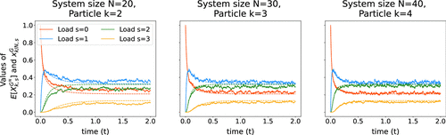
Notes. In each plot, the results for one system size are displayed. Throughout, the sample mean values are plotted against the values of the graphon mean field approximation.
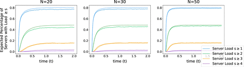
Note. The quantities are calculated as for the sample mean and for the approximation.
5.2. Heterogeneous Bike-Sharing System
5.2.1. Model.
We consider a bike-sharing model following the setup used in Fricker and Gast (2016) and Fricker et al. (2012). The model consists of bike stations, representing the particles in the system. Each station has finite capacity . The system has a fleet of bikes of size , which, at time , is evenly distributed among the stations, that is, bikes per station. The evolution of the system depends on the movement of bikes. We differ between the two cases; bikes in the system can either be stationary or in transit between stations. To align with the notations used in the theory part of the paper, we denote by the number of bikes at station i for time . For the system, heterogeneity comes from the varying popularity of stations. Hence, we denote by the popularity function. Based on the popularity function , we define the graphon of the bike-sharing system by . For the system of size N, connectivity for the stations is obtained by deterministic sampling as described in Section 3.2; that is, we discretize the graphon based on the system size N. For two stations , connectivity is, therefore, defined by . Based on the connectivity between stations, it remains to define the dynamics of the system. For a given state , the bikes move between stations in the following way:
Customers arrive at a station with rate leading to the transitions
The travel time of bikes between stations is exponentially distributed with rate . Hence, for station , the arrival rate of bikes is the product of the scaled popularity of station times the traveling bikes weighted by the travel time, that is, . This implies the transition
For the above, the notation refers to the unit vector of size N having a one at entry k and zeros everywhere else.
5.2.2. Drift and Limiting System.
To define the limiting system, we derive the drift implied by the above transitions and the defined graphon . We start by considering the indicator state representation as outlined in Section 2, that is, the drift is a vector of size of functions. In contrast to the stochastic rates, for the drift, the sum over particles is replaced by an integral over and the values of replaced by the graphon values. For a state with , the drift of the system at is defined by
By definition of the system and particularly the graphon, it is immediate that the assumptions of Theorem 1 and Corollary 1 hold, therefore guaranteeing the accuracy of the approximation.
5.2.3. Implementation and Results.
For our simulations, we set the popularity function of the bike-sharing system to . The travel rate and customer arrival rate are and , respectively. For the plots of Figures 4 and 5, we calculate the sample mean by averaging more than 7,500 simulations for each system size. For each plot in Figure 4, the mean field trajectory for a single item and state is plotted against the sample mean. Here, the horizontal axis represents time t and the vertical axis the probability for the item to be in the state. In Figure 5, a comparison of the sample mean against the values of the approximation for fixed time and state is shown. As used for the theoretical results, the state of the stochastic system is represented as a step function with constant value on the intervals for . In accordance with our theoretical results, the plot shows that, with increasing system size, the graphon mean field approximation becomes more accurate and captures the state distribution of the particles well.
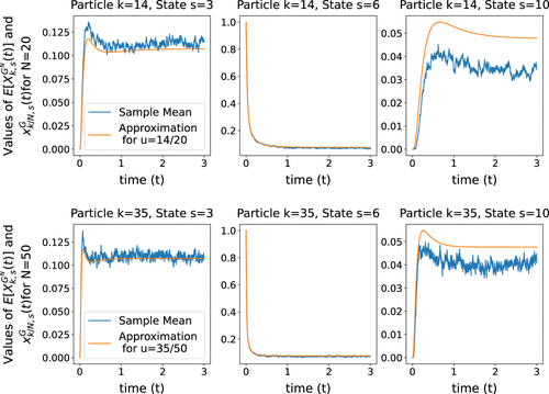
Note. The plots are generated for the states and .
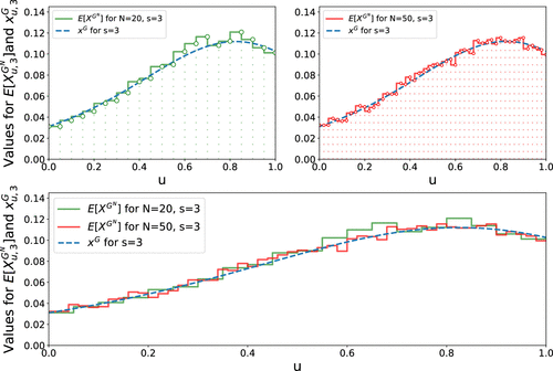
Notes. As for the main theorem of our results, we represent the values of the stochastic system as a step function with constant values on the intervals . The figure shows that, for increasing system size, the values of the stochastic system indeed approach the trajectory of the deterministic system. In the upper plots, the approximation is plotted against values of the sample mean for one system size each. In the lower plot, both functions are overlain for better comparison.
6. Proofs
This section provides the proofs of the main statements of this paper.
6.1. Proof of Lemma 2
We prove the uniqueness and continuous differentiability of the differential Equation (8) as well as the Lipschitz properties of the drift. The proof is the consequence of two lemmas:
We show in Lemma 3 that the drift is locally Lipschitz continuous in . By Driver (2003), this implies the existence of a local solution and the uniqueness of this solution.
In Lemma 4, we show that the directional derivatives of are well-defined and Lipschitz continuous. This property ensures that the is also continuously differentiable (for a proof of this property in general Banach spaces, see, for example, Driver 2003). □
(
Define , that is, we replace by under the integral. Applying the triangle inequality to the norm gives
Writing out the definitions and using the bounds of the rate vectors or matrices and the bound of the graphon, one immediately obtains
Last, we conclude that , where the and terms come from the vector and matrix notation used for the unilateral and pairwise rates as well as the sum over . □
(
Recall the definition of . We define for as in Equation (16). To see that is a directional derivative of in in direction , we show that it fulfills
Fix . By definition,
Dividing by and taking shows that is indeed a directional derivative of in . By definition, is linear in and as , and are bounded functions, the Lipschitz continuity in follows. □
6.2. Proof of Theorem 1
In the following, we present the proof of Theorem 1.
Let be the representation of the stochastic system as defined in Section 2.4. For a fixed , define
To compare the drift of the ODE against the drift of the stochastic process and ultimately bound them, we first want to rewrite , with being the quantity that fulfills for arbitrary with . In Online Lemma 5, we show that exists almost everywhere for and is almost everywhere equal to
In the above sum, is the directional derivative of in its initial condition in direction . We aim to bound the sum by using the properties of the derivative of and the differences between the drift of the deterministic and stochastic system with respect to the norm. The technical details to bound the remainder term and the difference between the drifts are moved to Online Lemmas 6 and 7. From the application of the latter lemmas, one obtains the bounds
6.3. Proof of Corollary 2 and Corollary 1
In this section, we prove the corollaries of Theorem 1. In each case, we use an additional lemma to obtain a bound on .
By the application of Theorem 1, we have
It, therefore, remains to bound the distance between the graphon G and graph . By application of Lemma 1 with probability at least and for large enough N
Defining and substitution into the above equation concludes the proof. □
The corollary is a direct implication of Theorem 1 and Online Lemma 8: because of representing a discretized version of G, it directly follows that is of order , which concludes the proof. □
7. Conclusion and Discussion
In this paper, we study an approximation for a system of particles interacting on a graph. We show that, when the interacting graph converges to a graphon, the underlying behavior of the stochastic system converges to a deterministic limit, which we call the graphon mean field approximation. Whereas this result is similar to other results in the literature—showing that graphon mean field approximations are asymptotically exact in some settings—our main contribution is to provide precise bounds on the accuracy of this approximation. We show indeed that the distance between the original finite-N system and the graphon mean field approximation can be bounded by a term that depends on the number of particles of the system plus a term that depends on the distance between the original graph and the graphon G when measured as an operator.
This paper aims to be methodological. It shows that it is possible to obtain bounds for a system with a graph structure and not mere asymptotic convergence results. To keep the presentation reasonable, we intentionally consider a relatively simple model, for instance, by restricting our attention to pairwise interactions between nodes or unilateral jumps and by considering that the rate functions are discretized versions of the limiting rates r. We believe that, by doing so, the proof is easier to follow and could then be adapted to more general cases. In particular, there are two direct follow-ups of this work.
First, the focus of this paper is to study the case of dense graphs that converge to graphons. This implies that the average degree of a node is linear in the number of edges. We believe that our methodology could be adapted in the not-so-dense case in which the average degree, say , goes to infinity at a sublinear rate. To do so, the scaling model should be changed: our model assumes that converges to G and that rates of transitions are of order . One needs to consider graphs such that converges to the graphon G and to have interaction rates of order . Once this is done, the part of our methodology that uses generators (Section 6.2 and Online Lemma 6) would still be applicable but would give us a rate of instead of . We believe that most of the rest of the proof (that concerns the Lipschitz continuity of the graphon mean field approximation) would continue to hold except for Lemma 1 (on stochastic sampling) that requires the average degree to be relatively large. For the case of sparse graphs, the number of neighbors per node remains bounded when the number of nodes N goes to infinity. This requires a fundamentally different approach: studying such a problem is out of the scope of our tools because the graphon mean field approximation is not asymptotically exact for sparse graphs.
Second, in this paper, we restrict our attention to finite-time convergence. We believe that, if the graphon dynamics has a fixed point that attracts all trajectories and one could bound the rate at which the convergence to this fixed point occur, then a bound on the steady-state convergence can be obtained, for instance, by adapting the methodology of Stein presented in Gast (2017) and Ying (2016). The main technical difficulty would be to adapt the perturbation theory from these papers to the case of the solution of the graphon mean field approximation.
The authors thank the anonymous reviewers for their insightful comments about the paper.
1 The constants hidden behind the big-O notation are essentially linear on the number of discontinuity points plus the Lipschitz constant.
2 In the literature, graphons are often restricted to symmetric functions because they are limits of undirected graphs. In our case, we allow the interactions between nodes to be asymmetric. We, therefore, allow for asymmetric graphon. Considering a symmetric or asymmetric function G would not change the proofs.
3 Here, is interpreted as a vector in .
4 For intricate intensity and graphon functions, it might be necessary to refine and tune the discretization approach.
5 Here, almost everywhere means that the property holds except on a subset of with measure zero.
References
- (2018) Community detection and stochastic block models. Foundations Trends® Comm. Inform. Theory 14(1–2):1–162.Google Scholar
- (2022) Mean field and refined mean field approximations for heterogeneous systems: It works! Proc. ACM Measurement Anal. Comput. Systems, vol. 6 (Association for Computing Machinery, New York), 1–43.Google Scholar
- (2022) Finite state graphon games with applications to epidemics. Dynam. Games Appl. 12(1):49–81.Google Scholar
- (2018) Centrality measures for graphons: Accounting for uncertainty in networks. IEEE Trans. Network Sci. Engrg. 7(1):520–537.Google Scholar
- (2021) Mean field interaction on random graphs with dynamically changing multi-color edges. Stochastic Processes Appl. 141:197–244.Google Scholar
- (2023) Graphon mean field systems. Ann. Appl. Probab. 33(5):3587–3619.Google Scholar
- (2024) Weakly interacting oscillators on dense random graphs. J. Appl. Probab. 61(1):255–278.Google Scholar
- (2019) Weakly interacting particle systems on inhomogeneous random graphs. Stochastic Processes Appl. 129(6):2174–2206.Google Scholar
- (2017) Stein’s method for steady-state diffusion approximations of M/Ph/n+M systems. Ann. Appl. Probab. 27(1):550–581.Google Scholar
- (2017) Stein’s method for steady-state diffusion approximations: An introduction through the Erlang-A and Erlang-C models. Stochastic Systems 6(2):301–366.Link, Google Scholar
- (2019) Supermarket model on graphs. Ann. Appl. Probab. 29(3):1740–1777.Google Scholar
- (2021) Graphon mean field games and their equations. SIAM J. Control Optim. 59(6):4373–4399.Google Scholar
- (2012) Large graph limit for an SIR process in random network with heterogeneous connectivity. Ann. Appl. Probab. 22(2):541–575.Google Scholar
- (2023) Individual based SIS models on (not so) dense large random networks. Preprint, submitted February 26, https://arxiv.org/abs/2302.13385.Google Scholar
- (2003) Analysis tools with applications. Lecture notes. https://mathweb.ucsd.edu/∼bdriver/240-01-02/Lecture_Notes/anal.pdf.Google Scholar
- (2016) Incentives and redistribution in homogeneous bike-sharing systems with stations of finite capacity. EURO J. Transportation Logist. 5(3):261–291.Google Scholar
- (2012) Mean field analysis for inhomogeneous bike sharing systems. Proc. 23rd Internat. Meeting Probabilistic Combin. Asymptotic Methods Anal. Algorithms (Montreal, Canada).Google Scholar
- (2022) Non-Markovian interacting particle systems on large sparse graphs: Hydrodynamic limits and marginal characterizations. Unpublished PhD thesis, Brown University, Providence, RI.Google Scholar
- (2024) Hydrodynamic limits of non-Markovian interacting particle systems on sparse graphs. Electronic J. Probab. 29:1–63.Google Scholar
- (2017) Expected values estimated via mean-field approximation are 1/N-accurate. Proc. ACM Measurement Anal. Comput. Systems 1(1):1–26.Google Scholar
- (2017) A refined mean field approximation. Proc. ACM Measurement Anal. Comput. Systems 1(2):1–28.Google Scholar
- (2023) Universality of sis epidemics starting from small initial conditions. Preprint, submitted August 16, https://doi.org/10.2139/ssrn.4543174.Google Scholar
- (1970) Solutions of ordinary differential equations as limits of pure jump Markov processes. J. Appl. Probab. 7(1):49–58.Google Scholar
- (1971) Limit theorems for sequences of jump Markov processes approximating ordinary differential processes. J. Appl. Probab. 8(2):344–356.Google Scholar
- (2007) A generic mean field convergence result for systems of interacting objects. Fourth Internat. Conf. Quant. Evaluation Systems (IEEE, Piscataway, NJ), 3–18.Google Scholar
- (2012) Large Networks and Graph Limits, Colloquium Publications, vol. 60 (American Mathematical Society, Providence, RI).Google Scholar
- (1967) Propagation of chaos for a class of non-linear parabolic equations. Stochastic Differential Equations, Lecture Series in Differential Equations, Session 7, Catholic University, 41–57.Google Scholar
- (2001) The power of two choices in randomized load balancing. IEEE Trans. Parallel Distributed Systems 12(10):1094–1104.Google Scholar
- (1972) Markov Processes and Learning Models, vol. 84 (Academic Press, New York).Google Scholar
- (2022) Beyond mean-field limits for the analysis of large-scale networks. Queueing Systems 100(3–4):345–347.Google Scholar
- (2023) Recent advances in modeling and control of epidemics using a mean field approach. Sādhanā 48(4):207.Google Scholar
- (2023) Mean-field analysis for load balancing on spatial graphs. Proc. 2023 ACM SIGMETRICS Internat. Conf. Measurement Model. Comput. Systems (Association for Computing Machinery, New York) ,27–28.Google Scholar
- (1986) Approximate computation of expectations. Lecture Notes-Monograph Ser. 7:i–164.Google Scholar
- (2017) Random Graphs and Complex Networks (Cambridge University Press, Cambridge, UK).Google Scholar
- (2020) Graphon-based sensitivity analysis of sis epidemics. IEEE Control Systems Lett. 4(3):542–547.Google Scholar
- (2016) On the approximation error of mean-field models. ACM SIGMETRICS Performance Evaluation Rev. 44(1):285–297.Google Scholar
- (2024) Optimal rate-matrix pruning for heterogeneous systems. ACM SIGMETRICS Performance Evaluation Rev. 51(4):26–27.Google Scholar
- (2024) Exploiting data locality to improve performance of heterogeneous server clusters. Stochastic Systems 14(3):229–272.Link, Google Scholar