Generalized Max-Weight Policies in Stochastic Matching
Abstract
We consider a matching system where items arrive one by one at each node of a compatibility network according to Poisson processes and depart from it as soon as they are matched to a compatible item. The matching policy considered is a generalized max-weight policy where decisions can be noisy. Additionally, some of the nodes may have impatience, that is, leave the system before being matched. Using specific properties of the max-weight policy, we construct a simple quadratic Lyapunov function. This allows us to establish stability results, to prove exponential convergence speed toward the stationary measure, and to give explicit bounds for the stationary mean of the largest queue size in the system. We finally illustrate some of these results using simulations on toy examples.
Funding: N. Soprano-Loto is partially supported by Aristas, MathAmSud [Grant RSPSM (Random Structures and Processes in Statistical Mechanics)], and ANR (Agence Nationale de la Recherche) [Grant PRC (Projets de Recherche Collaborative) MATCHES (CE40)].
1. Introduction
The so-called bipartite stochastic matching model was introduced in Caldentey et al. (2009) (see also Adan and Weiss (2012) and Adan et al. (2017)) as a variant of skill-based service systems. In this model, two infinite ordered sequences (a sequence of servers and a sequence of customers) are considered, and customer/server are matched in first come, first served order, that is, from left to right, according to compatibilities that are prescribed by a given bipartite graph. In the so-called extended bipartite matching model (Bušić et al. 2013), customer/server couples enter the system at each time point. A matching occurs when an arriving customer (respectively, server) finds a compatible server (respectively, customer) present in the system, in which case both leave the system instantaneously. Otherwise, items remain in the system waiting for compatible arrivals (in particular, there are no service times). The field of applications of such models is very wide, from housing to job applications, from transplant protocols to blood banks, peer-to-peer systems to dating websites, ride sharing, and so on. The mathematical settings of such models are the following: there is a set C of customer classes and a set S of server classes, and a bipartite graph on the bipartition indicates the compatibilities: a customer class and a server class are compatible if and only if there is an edge between nodes c and s in the compatibility graph. Customer/server couples enter the system in discrete time (or are read one by one from left to right, in the prior models), and the classes of the couples in the order of arrivals (respectively, read from left to right) are independent and identically distributed (i.i.d.) from a measure μ on C × S. In Caldentey et al. (2009), Adan and Weiss (2012), and Adan et al. (2017), it is assumed that on C × S; that is, the class of the incoming customer and server are independent of one another, whereas this assumption is relaxed in Bušić et al. (2013). In case of multiple compatibilities, it is the role of the matching policy to determine what match is performed. In Adan et al. (2017), it is shown that, under a natural stability condition, the stationary probability of the system under first come, first served has a remarkable product form. Interestingly, this result can then be adapted to various skill-based queueing models as well and in particular those applying (various declinations of) the so-called first come first matched (FCFM)-assign the longest idling server (ALIS) service discipline (Adan and Weiss 2014). For various extensions of bipartite matching models, see also Adan et al. (2018). In Bušić et al. (2013), the stability condition in Adan et al. (2017) is shown to be also sufficient for the stability of extended bipartite models ruled by the “match the longest” policy, consisting of always matching incoming items to the compatible class having the longest queue. In Moyal et al. (2018), a coupling from the past result is obtained, showing the existence of a unique bi-infinite matching in various cases of extended bipartite matching models and for a broader class of matching policies than FCFM, thereby generalizing various results of Adan et al. (2017).
In many practical systems, it is often more realistic to assume that arrivals are simple instead of pairwise. Moreover, the bipartition of the compatibility graph into classes of servers and customers only suits applications in which this bipartition is natural (donor/receiver, house/applicant, job/applicant, etc.). However, in many cases, the context requires that the compatibility graph take a general (i.e., not necessarily bipartite) form. For instance, in dating websites, it is a priori not possible to split items into two sets of classes with no possible matches within those sets. Similarly, in kidney exchange programs, intraincompatible donor/receiver couples enter the system looking for a compatible couple to perform a crossed transplant. Then, it is convenient to represent donor/receiver couples as single items, and compatibility between couples means that a kidney exchange can be performed between the two couples (the donor of the first couple can give to the receiver of the second, and the donor of the second can give to the receiver of the first). In particular, if one considers blood types as a primary compatibility criterion, the compatibility graph between couples is naturally nonbipartite. Motivated by such applications, among others, Mairesse and Moyal (2016) proposed a generalization of the previous matching models, termed general stochastic matching model, in which items enter one by one, and the compatibility graph G is general. For a given compatibility graph G and a given matching policy , the stability region Stab of this system is defined as the set of those measures μ deciding the class of the incoming items, such that the Markov chain describing the evolution of the system is positive recurrent. Mairesse and Moyal (2016) identified a universal necessary condition for stability, that is, a set Ncond(G) that includes Stab for any matching policy and any graph G. Following Bušić et al. (2013), Mairesse and Moyal (2016) also showed that match the longest is maximal stable; that is, it has a maximal stability region, as the two sets Ncond(G) and Stab coincide. Moyal and Perry (2017) then showed that, aside for a particular class of graphs, the random class-uniform policy (choosing the match in a compatible class of the incoming item, uniformly at random among those having a nonempty queue) is never maximal stable and that priority policies are in general not maximal stable. Then, Moyal et al. (2020) showed that the policy first come, first matched is maximal stable and that, similarly to Adan et al. (2017), the stationary probability of the system can be written in a product form. Various extensions of the general stochastic matching model can also be found in Büke and Chen (2015, 2017) regarding systems with bipartite complete compatibility graphs but in which each match can be enacted with a nominal probability, and in Rahmé and Moyal (2019) to stochastic matching systems on hypergraphs, thereby matching items by groups of two or more. In a recent line of study, stochastic matching models have also been studied from the point of view of stochastic optimization (Gurvich and Ward 2014, Bušić and Meyn 2016, Nazari and Stolyar 2019). In particular, the max-weight policy introduced in Tassiulas and Ephremides (1992) is a natural policy allowing a natural tradeoff between efficiency and stability.
Here we consider a matching system where items arrive one by one at each node of a compatibility network according to Poisson processes and depart from it as soon as they are matched to a compatible item. The matching policy considered is a generalized max-weight policy where decisions can be subject to noise. Additionally, some of the nodes may have impatience, that is, leave the system before being matched.
1.1. Motivation
In many applications, reneging of items needs to be taken into account: for instance, applicants may renege from the systems, whereas jobs/houses/university spots may no longer be available. Similarly, in organ transplants, patients may renege from the system because of death or change in their diagnosis, whereas organs have a short life duration outside a body and need to be transplanted within a very short period of time—see a first approach of such systems in Boxma et al. (2011).
The present work is dedicated to an extension of general stochastic matching models to the case where (i) classes of items can be impatient, in that they renege from the system if they do not find a match within a given (random) period of time, and (ii) the matching policy is of the max-weight class, with possible errors in the assessment of the system state.
Specifically, we consider that the policy decisions may be subject to noise that can lead to errors in the estimate of the queue lengths, which is necessary to implement matching policies of the max-weight type.
Indeed, as is well known from the vast literature on the load balancing of parallel service systems, implementing policies that are sensitive to the queue sizes, such as the max-weight type policies considered in the present paper, becomes algorithmically prohibitive as the number of queues grows large. Efficiently sorting the queue sizes may easily lead to inaccuracies, entailing routing errors.
Specifically, in many practical cases the queue sizes of the various servers are not always known: they are either estimated by the incoming customers (as in physical queues in supermarkets, for instance), or by a central dispatcher (e.g., in passport-checking stations). Likewise, information regarding the queues to each of the servers in large web-server farms or call centers require constant communication between the job dispatchers and the servers, slowing down the response time. This information is thus not always available in real time (Lu et al. 2011), and in such cases, it can then be preferable to estimate the queue sizes, based on past or partial information, for instance. Observe that this source of inaccuracies is the main motivation for introducing “Power of d”–type policies to reduce the complexity of routing and the probability of errors by routing the requests only to a subset of the available servers having a more tractable size (see Mitzenmacher (1996) and related references on this matter).
In the context of matching systems, in most of the aforementioned applications, the requests of the various classes are physically gathered in different queues; that is, each node of the graph has its own buffer for storing the corresponding items. In many cases, the size of the graph, that is, the number of classes, is large, leading to routing problems that are similar to the context of parallel service systems. For instance, liver transplants are subject to compatibility constraints that lie far beyond the blood types of givers and receivers, namely, age, the nature of the pathology of the patient (cancer or cirrhosis), and immunological criteria. This leads to an increase of the number of classes of givers and receivers, and in turn, to an increase of the complexity of implementing max-weight type policies and to the potentiality of allocation errors or inaccuracies.
To account for this difficulty, in the spirit of Moyal and Perry (2021) for parallel service systems, we introduce an error parameter in the estimate of the queue sizes in the context of matching systems. In this context, it is then reasonable to consider that these errors are independent of one another but follow distributions that may depend on the specificity of the considered nodes. For instance, an arriving item to node j chooses a match from the neighboring node i, making an error of estimate of the queue length of node i, that may depend on i and j; see our later assumptions.
All in all, by “generalized max-weight policies,” we mean policies that are sensitive to the queue sizes, that incorporate rewards to give specific weights to the various matchings, and that take into account the possibility of errors in assessing the queue sizes of the various nodes of the graph.
1.2. Main Contributions
As we developed previously, the extension of the general stochastic matching model introduced in Mairesse and Moyal (2016), to the paradigm of reneging systems, is prevalent in practice. As will be specified later, adding an impatience parameter (possibly to some, but not all of the item classes) makes the analysis more intricate than in the original model. This constitutes the first main contribution of this work.
Using the specific structure of the max-weight policy, our second main contribution, Theorem 1, is to show that a simple quadratic function is a Lyapunov function whenever the traffic condition “” (see (4)) that can be understood as a generalization of the classical condition “” to the case of reneging, is satisfied. This result is interesting and original for its own sake, even in the no-reneging case. This allows us directly to characterize the stability region and, as a corollary, to conclude that the max-weight policy is maximum stable. By doing so, we widely generalize results in Mairesse and Moyal (2016) to the case of generalized max-weight policies (of which the match the longest (ml) policy introduced in Bušić et al. (2013) and then Mairesse and Moyal (2016) is a particular case, see the later discussion) and to matching models with reneging. This quadratic function was already identified in Mairesse and Moyal (2016) and Bušić et al. (2013) as a Lyapunov function by an indirect proof: First, by stating that if the Foster-Lyapunov criterion applies to a quadratic Lyapunov function for some matching policy, then it must be also the case for the policy ml, and second, by showing that the criterion does apply to an ad hoc randomized policy. However, this argument cannot be generalized to the much wider case of max-weight policies, whence the main interest of the direct proof that is presented here.
We say that a couple graph/reneging vector is stabilizable whenever there exists a matching policy and an arrival vector λ making the corresponding matching model stable. As a consequence of Theorem 1, is stabilizable if and only if the set is nonempty. It is well known (theorem 1 in Mairesse and Moyal 2016) that for a general stochastic matching model without reneging, the graph G is stabilizable if and only if it is not bipartite, because this condition is equivalent to being nonempty. Our third main contribution is a quite remarkable result: In Proposition 2, we show a very simple sufficient condition for the stabilizabiliy of the system: it is sufficient that G be nonbipartite, or that only one class of elements renege. In particular, for a bipartite G (as is the case for organ transplants model, for instance), the system is stabilizable if, and only if at least one class of elements renege. Said differently, whenever G is bipartite and arrivals are made by single items, it is enough that one node receives impatient elements to make the system stabilizable, rather than artificially assuming that arrivals are made by pairs (as is the case in the (extended) bipartite matching models studied in the literature).
Showing that a given (even simple) function is a Lyapunov function is in general a challenging issue, and our case is not an exception, especially in such general a context. Our proof is quite intricate and relies on carefully exploiting this generalized Ncond condition. Combining these ideas, as our fourth main contribution, we are also able to prove exponential convergence speed toward the stationary measure, and additionally, by combining with stochastic comparisons, to construct bounds for the stationary mean of the largest queue size of customers in the system.
We finally illustrate some of those results using simulations on toy examples.
1.3. Outline of the Paper
In Section 2, we give the formal definition of the model we study. Section 3 is dedicated to the theoretical results. Section 3.1 focuses on stability: we characterize the stability region of the models in Theorem 1; this theorem is based on Proposition 1, a key result in which we control the drift of a quadratic function. Last, Proposition 2 describes precisely whether a given model is stabilizable. In Section 3.2, we then investigate the speed of convergence to equilibrium: a geometric Lyapunov bound is given in Proposition 3, and the exponential convergence to equilibrium follows as a consequence in Theorem 2. In Section 3.3, some bounds are given for moments of the size of the largest queue of the system in equilibrium in Theorem 3. Section 4 is dedicated to simulations: we compare the max-weight policy with a priority policy in Section 4.1, and an analysis of the theoretical bounds obtained in the previous section is given in Section 4.2. All proofs are provided in Section 5.
2. Model
2.1. Notation
The graph is assumed in all the article to be finite, simple, undirected, and connected. Because the set of nodes V represents customers classes, we use the words node and class in an indistinguishable way during all the article. The nonconnected case can be addressed by decomposing into connected components. Furthermore, to avoid trivialities, we assume . We write to denote that there is an edge connecting the nodes in the graph G. We say that a subset is an independent set if implies . For any subset , we let
2.2. Stochastic Matching Model with Reneging
The (continuous-time) stochastic matching model with reneging is formally defined as follows: we give ourselves a set of independent Poisson processes , of respective intensities , and denote by the arrival intensity vector of the model. For any , we denote by the sequence of successive arrival times in the process N(i). For any subset , denote by the intensity of the superposed Poisson processes having indexes in W. The overall superposition of the Poisson process of the N(i)s, , is denoted by N. It is thus a Poisson process of intensity , and its points are denoted by . For all i, on each point , an item of class i (or i-item for short) enters the system. Thus, the points of N are the overall arrival times in the system. We say that two items of respective classes i and j in V are compatible if and only if . To each class is also associated a parameter . Denote , the reneging rate vector of the model. Unlike the vector λ, we allow γ to have null entries. We then associate to each i-item an exponential random variable (r.v.) of distribution , interpreted as its patience time. An r.v. of distribution is interpreted as almost surely (a.s.) infinite, and we denote by
The dynamics of the model is then defined recursively at the successive points of N, as follows:
We start at time 0 with a state in which all present items are incompatible. In other words, in the system at time 0, for any , there are either no i items, or no j items, or neither. Such a buffer content is called admissible. We associate a patience to each of these initial items that is drawn, independently of everything else, from the distribution corresponding to its class, for example, from () for a j-item. As previously mentioned, if , that is, , the patience time of the corresponding item is set as infinite.
Let , and suppose that the buffer content of the system was admissible at time . We first update the buffer content at each reneging time in , by discarding all items present in the system at time and whose patience time has expired during that time interval. Observe that the buffer content remains admissible after this procedure. Then, suppose that Tn is a point of the jth arrival process, that is, for some , or in other words, a j-item enters the system at Tn. This happens with probability
(1)We then face the following alternatives:
(a) Either the buffer contains no items compatible with the incoming j-item, that is, there are no stored items of classes in E(j), in which case the latter item is stored in the buffer. We then draw the (possibly infinite) patience time of this item from the distribution (), independently of everything else.
(b) Or there is at least one remaining item having class in E(j) in the buffer. Then the incoming j-item must be matched with one of these compatible items, and it is the role of the matching policy to determine its match. We assume that the matching policy is of the generalized max-weight policy type with parameters w and F (mw, or simply mw, for short). To define this, let be a family of nonnegative numbers and be a family of cumulative distribution functions (c.d.f.s). We index with ordered pairs instead of the unordered ones because the involved parameters are not assumed to be symmetric. The first entry of the pair j will typically represent the class of the incoming item, and the second one i, the class of the item j performs a match with. Denote, for all , by x(i) the number of stored i-items at this time. Then the match of the incoming j-item is chosen uniformly at random from the set
(2)where is an r.v. drawn at time n independently of everything else from the c.d.f. , interpreted as the measurement error of the queue length of node i, made on an arrival of a j element at time Tn, and is interpreted as the specific reward of matching an incoming j-item with an i-item. Observe that in (2), we make the simplifying assumption that measurement errors are made only regarding the length of nonempty queues; that is, empty queues are identified correctly. This makes sense in practice, first, because the overestimation of the size of an empty queue might lead to a matching involving an item that is not actually present in the system. Second, it is usually simpler to determine whether a given buffer is empty or not (by sending a ping to the corresponding server) than to precisely measure the size of a (potentially much longer) nonempty queue.Then, once the matching is done, the incoming j-item leaves the system right away, together with its match. We emphasize that, unlike the notion of compatibility given by the undirected set of edges E, symmetry between i and j is a priori not assumed in the definitions of the measurement errors and the matching rewards.
It is then easily seen that, in any case, the buffer content at time Tn is also admissible.
We continue the construction inductively.
Particular cases of generalized max-weight policies are as follows:
The classical max-weight policies, as defined inTassiulas and Ephremides (1992), recovered by taking constant weights and, for every such that , the c.d.f. as the one corresponding to the Dirac δ0 distribution, that is, no error.
The match the longest policy introduced inMairesse and Moyal ( 2016), recovered by taking and for all such that , that is, no measurement errors and no rewards.
The error measurement model we consider is additive, namely, a scale-free error is made on all queue lengths, and we prevent absurd measurement of negative queue lengths by taking the positive part of the latter (see (2)). Another interesting model would be to assume mutliplicative error measurements; namely, (2) would read
We strongly believe that all results to come also hold in that case but leave the proof of this conjecture to the reader.
2.3. Markov Representation
Let, for all be the queue length vector at time t, namely, for any is the number of i-items in the buffer at time t. It is easily seen that the process is a regular continuous time Markov chain (CTMC) on the (countable) commutative state-space
For any , let be its support. Observe that Sx is an independent set for every . For all , denote by δi the ith canonical vector: . The infinitesimal generator of X is then simply given by
3. Results
3.1. Stability
The state is said to be positive recurrent if the expected amount of time until the CTMC revisits x given that , is finite. The CTMC is said to be positive recurrent if every state is. Because the CTMC is irreducible, this occurs if and only if some state is positive recurrent. Positive recurrence is equivalent to the existence and uniqueness of an invariant distribution. We say that the matching model is stable if the CTMC is positive recurrent. The next result provides a necessary and sufficient condition for stability.
For any connected graph G and any , the model is stable if and only if its intensity vector λ belongs to the set
Observe that if we define
For , let be an r.v. with c.d.f. given by ; that is, has the same distribution than for every n. For , define
The quantity is tailor-made for the event
Theorem 1 is a corollary of the following key generator bound for a quadratic function.
Assume and let . Let be the quadratic function defined by , and let .
If , then
(6)for every .Otherwise, if , we have
(7)for every .
As can be easily seen in the proof of the necessity statement in Theorem 1, for a connected graph G and a reneging rate vector γ, λ being an element of is necessary for the existence of a matching policy that makes the system stable, whatever the matching policy is. The sufficiency statement means that such models always exist whenever λ do belong to —It suffices to implement a matching policy in the max-weight class. Therefore, it is natural to say that the couple is stabilizable if there exists an intensity vector λ such that the model with reneging is stable, that is, if Ncond is nonempty. The following proposition makes precise the class of stabilizable graphs.
Let be a connected graph and be a reneging rate vector. Then is nonempty if and only if G is nonbipartite or .
In other words, if G is bipartite, it is enough that one class of elements renege to make the system stabilizable. As will be made clearer in the proof of Proposition 2, the reason behind this (apparently surprising) result is as follows: if is bipartite, say of bipartition , and no elements renege, then the only independent set I that cannot satisfy for some intensity vector λ is either I = V1 or I = V2 because, as G is bipartite and connected, is the only pair of sets such that and , and we cannot have together with . Then, adding reneging to a single node of V1 (if I = V1), or to V2 (if I = V1) allows to simply break this paradoxal symmetrical condition. See the details in Section 5.3.
To summarize, gathering Theorem 1 and Proposition 2, we obtain the following panorama regarding the stability of the model:
Any couple is stabilizable provided that G is nonbipartite or that some classes of elements renege, that is, .
Under these conditions, any model with , is stable.
(Full Reneging Case). In the case where , that is, all items may renege, Condition (4) is empty, and we retrieve the good-sense result that any such matching model is stable, whatever the intensity vector λ.
(No-Reneging Case). In the case where (no reneging), the model amounts to a continuous-time version of that introduced inMairesse and Moyal (2016). From Theorem 1, any model is stable whenever λ belongs to the set
In other words, any policy of the mw type is then maximal stable, in the sense that it has the largest stability region. This result generalizes those ofMairesse and Moyal (2016). Indeed, setting for all (j, i) (no errors) and for all and all (equal rewards for all matches involving an incoming j-item, ), the matching policy amounts to match the longest (priority is given to the node having the largest queue), and we retrieve assertion (15) in theorem 2 ofMairesse and Moyal (2016). Theorem 1 is thus a wide generalization of the latter result, to the case of weighted mw policies with measurement errors.
3.2. Speed of Convergence to Equilibrium
In this and the following section, we assume for simplicity. The involved techniques can be used to obtain analogous results in the general case (see Remark 5).
Building on the previous results and following classical approaches for Markov processes with bounded jumps, we now show how to define a geometric Lyapunov function that is very useful to quantify the speed of convergence to the steady state. We first have the following result.
Let be a max-weight stochastic matching model with and λ belonging to the set defined by (4). Then, if is small enough, there exist such that
The previous proposition implies that the distribution of the Markov process X converges to its stationary distribution exponentially fast. More precisely, the following result follows immediately from Proposition 3, using, for example, the results in Hairer (2014).
As in Proposition 3, let be a max-weight stochastic matching model with and λ belonging to , and let π be the unique invariant distribution of the process X (granted by Theorem 1). For any there exist constants c > 0 and such that
3.3. Moments Bounds at Equilibrium
We control below the first moment of the maximum queue size under the steady state of the system.
Assume that we are under hypotheses of Proposition 3, namely and , and let π be the unique invariant distribution. Let have distribution (this r.v. has been defined in Section 3.1), and assume that there exists such that for every such that . Then we have that
With exactly the same procedures, the content of Sections 3.2 and 3.3 can be extended in the following two directions: on the one hand, one may weaken hypothesis ; on the other, bounds for higher order moments under π may be obtained. We prefer to avoid developing this direction since the computations become rapidly cumbersome.
4. Simulations
In this section, we present a few simulation results. In the first set of simulations, we illustrate the gain of performance of max-weight policies with respect to other, more static, policies, for systems with reneging. To do so, as an illustrative example, in Section 4.1, a max-weight policy is compared with policies of the priority type, namely, policies that only take into consideration the rewards of the various matches but not the queue sizes. Then, in Section 4.2, we compare the theoretical bounds obtained by Lyapunov techniques in Section 3.3 with simulated values. These bounds are not meant to be very tight, and we leave their optimization for future research.
4.1. Comparison with Priority Policies
In this section, we assume for every such that , namely no measurement errors are considered. A policy is said to be of the priority type if, whenever the system is in state and a j-item enters the system, the match of the incoming j-item (if any) is chosen uniformly at random from the set
This amounts to saying that each j-item has a fixed order of priorities between the neighboring nodes of i, for choosing its match. (Observe that a priority policy can be seen as a max-weight policy where we set the errors to a.s. for all n, (j, i).) As it is illustrated in the two examples in section 5 of Mairesse and Moyal (2016), priority policies can be maximal stable or not. Conversely, as is shown in theorem 3 of Moyal and Perry (2017), for any graph G outside a particular class of graphs, there always exists a nonmaximal priority policy.
To compare the asymptotic behavior of max-weight and priority policies for a variety of graphs, arrival and departure rates, and rewards, we randomize all these parameters. We perform 100 simulations. In each one, we first sample the graph G, the arrival rates λ, departure rates γ, and rewards w, as follows:
The graph is an Erdős-Rényi one with parameters and ;
The arrival rates are i.i.d. with common distribution ;
The reneging rates are i.i.d. with common distribution (on average, half of the nodes do not renege); and
We consider symmetric rewards, namely for every i, j such that , and the family is i.i.d. with common law .
In each case, the condition Ncond is forced; that is, if λ is not an element of Ncond(G), the simulation is rerun. Then, for each simulation we compare a system ruled by max-weight to the same system ruled by the corresponding priority policy, for the same sampled parameters. In other words, we perform paired replications in the sense that a random network is generated by items 1–4, and the same network is used for comparing the corresponding policies. Two level of randomness are involved: the first one to define the network (formed by the graph, and the values of the rates and rewards), and the second one to draw, conditioned to the already sampled network, the effective dynamic of the process (consisting on the arrival and departure episodes, and the randomness to decide which item class to pick in case of a tie in the value of the weights). Observe that, from Theorem 1, the max-weight system is necessarily stable, whereas in view of the previous observations, the system ruled by the priority policy is not necessarily so.
Figure 1 represents, in vertical order, the size of the largest queue, the cumulative reward (each time a -match occurs, a reward accumulates) and the cumulative number of departures, the three quantities versus time, in the time interval . Figure 2 is the boxplot for the size of the largest queue at time t = 100.
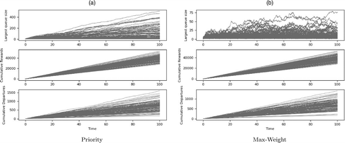
Notes. (a) Priority. (b) Max-weight.
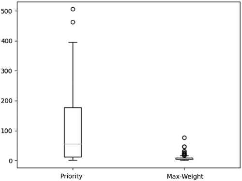
These results put in evidence an important and striking qualitative difference between the two policies, in the behavior of the buffer size process. Specifically, max-weight keeps far fewer items in the system, whereas both policies have essentially the same performance in terms of cumulative reward and departures. In many cases, the priority policy seems to fail in stabilizing the system, whereas the corresponding max-weight system is always stable. Finally, it is worth mentioning that the same picture was obtained in unpublished simulations ran in much larger time intervals.
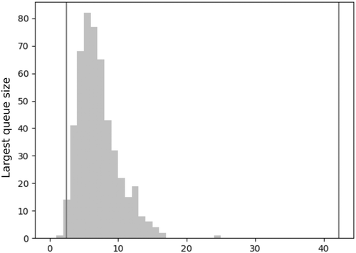
4.2. Bounds in the Stationary Regime
Unlike Section 4.1, in this section, impatience is excluded. We first restrict our attention to the classical match the longest policy; that is, we take for every such that , and we work without measurement errors. An important difference with respect to the previous subsection is that here the parameters are drawn only once at the beginning. We clarify that no comparison with a priority policy is made here. The distribution of the pair is maintained: Erdős-Rényi distribution with parameters and for G, and common distribution for the i.i.d. family . Figure 3 represents a histogram at time t = 100 of 500 simulations. The vertical lines represent the lower and upper bounds for the expected size of the largest queue given by Theorem 3.
Finally, we study the case with measurement errors and rewards. The random variables giving place to the noises are chosen to be i.i.d. with common distribution , and the rewards are again symmetric and i.i.d. with common distribution . The distributions of G and λ do not change, and the tuple is drawn only once at the beginning. Figure 4 is a histogram also for 500 iterations at time t = 100, and the vertical line represents the lower bound for the expectation. The numerical value for the upper bound for the expectation is 26,867.96, and it is not included in the graphic.
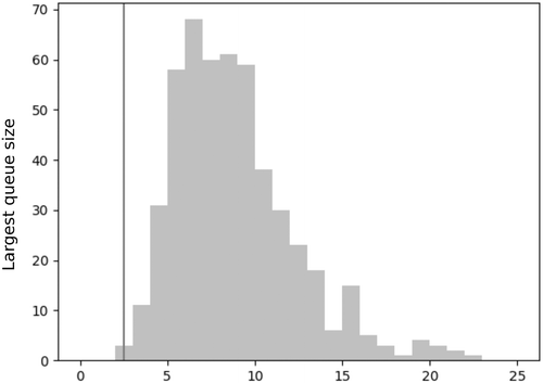
For match the longest, we observe tight bounds for the expected value. All the upper bounds become very loose when we include the presence of rewards or noises. From unpublished simulations, we observe that this is a general picture and not only a particular situation for this choice of the parameters. In the presence of asymmetric rewards and noise, the bounds are not informative. We leave for future work to obtain better tailored made bounds in this case. A typical histogram is very close to the lower bound for the expectation, and the upper bound is more accurate if larger values of p in the distribution of G are considered.
5. Proofs
5.1. Proof of Proposition 1
Fix and . To shorten notation, we write
We assume during the proof that we are in the th step, namely, the law of is ruled by the family of r.v.s ; of course, by homogeneity, this can be done without loss of generality. For the quadratic function f2, identity
Because for all , the first sum equals
Observe that
Putting these observations together, we get
From now on the proof is devoted to controlling the last term; an objective that will be carried out through the use of the following technical result.
Fix and , and assume that the nonempty subset satisfies the following hypotheses:
For every .
For every .
Then
In the assumptions of Lemma 1, hypothesis 1 states that, conditioned to , an arriving j-item necessarily matches with an item whose class belongs to W. On another hand, hypothesis 2 states that the inequalities defining Ncond are satisfied inside the set W. The connection between the two hypotheses can be informally understood as follows: the second one gives stability inside W, and the first one tells you that this stability is not being taken advantage of by classes outside .
Before providing the proof of Lemma 1, we show how to conclude from it. To avoid trivialities, we assume from now on.
Assume (no reneging). It is easy to see that the hypotheses of Lemma 1 are satisfied for . Hence, from (13) it follows that
(14)Then simply replace in (12) to obtain the desired inequality (6).
We now turn to the case where . First, the result in the subcase follows immediately from (12). Therefore, let us finally assume that and . Coming back to (12), we have
(15)
If , we can easily conclude because
From now on we assume that , and we recall that we are in the situation in which and . One is tempted to apply Lemma 1 with , especially because, for this particular choice of W, hypothesis 2 of this lemma is guaranteed by the hypothesis . Unfortunately, hypothesis 1 of Lemma 1 fails. The rest of the proof is devoted to finding a proper subset fitting this missing requirement.
Here we introduce a crucial notion of connectivity that depends on the number of stored items, notion that is also used in the proof of Lemma 1. We define an auxiliary graph by setting and . Let be the partition of induced by the connected components of the graph : for every , C is a subset of , and every pair is connected by a path of edges in . The set
We first see that . Let be such that , and let be the subset to which i0 belongs. We will prove that . We have to see that for every . If , this follows because
(17)If , consider a path in connecting i0 with i, namely, take (L is simply the length of the path) such that for every , and for every . The definition of C0 implies that
(18)Using that , we have
as desired.We prove now that hypothesis 1 of Lemma 1 holds. For fixed, we have to see that, conditioned to , the policy necessarily performs a match with an item class in W. This follows if we prove that
(19)for every and . We split into the following two subcases: and .(a) If , we have
(b) For the subcase , we will use the following obvious property: if both belong to the same set of connected nodes , and is such that , then also i3 belongs to C. We next show that
(20)
Suppose by contradiction that the inequality is false. Let be the subset to which belongs, and let be such that (such an exists because otherwise would belong to W). In particular,
The mentioned property implies that , contradictorily implying that . Once we have Inequality (20), we can conclude because
(21)As mentioned before, hypothesis 2 of Lemma 1 holds for because of the assumption, and it extends to W simply for being a subset.
We can now apply Lemma 1 to W, use that for every , and use that , to obtain
Replace in (15) to conclude.
We divide the proof into three steps.
Step 1: Separation into connected components. We define an auxiliary graph by , and we denote by the partition of W into connected subsets of nodes. We suppose that they are ordered in a decreasing way with respect to the number of stored items: if , and if and , then . More precisely, if is an enumeration of the nodes in W such that for every , there are exactly of them such that for every , and they satisfy and . The idea behind these definitions is to distinguish nodes whose weights are too far apart. In particular, we will use the following property:
In other words, conditioned to , an incoming item whose class belongs to necessarily matches with an item whose class belongs to . To see why this is true, take . In particular, we have , so by hypothesis; hence, we are done if . The case follows because, for every and every , we have
We will also use that
Step 2: Control of the number of stored items in each Cl. In this step, we reduce the problem by controlling the maximum and minimum number of stored items belonging to the same connected subsets. First observe that
However, observe that
Step 3: Iterative procedure. First, recalling (5), observe that
In the last inequality, we used hypothesis 2; in the second identity, we use Property (22). We are in the following alternative: if it holds that
However, as in (29), we have that
5.2. Proof of Theorem 1
Necessity of the condition Ncond can be shown similarly to proposition 2 in Mairesse and Moyal (2016): For any and any , all items of class in I that have departed the system before t have necessarily been matched with an element of E(I) arrived before t; thus, we have that
We now prove sufficiency. By the continuous-time version of the Foster-Lyapunov theorem (Meyn and Tweedie 1993), it suffices to show that
5.3. Proof of Proposition 2
To expedite the proof, first observe that, for any G and γ, is an element of defined by (4) if and only if defined by (1) is an element of
First, if G is bipartite and , then theorem 1 of Mairesse and Moyal (2016) shows that the set is empty. From the previous remark, so is the set .
Regarding the converse, let us first assume that G is nonbipartite. Then, again from theorem 1 in Mairesse and Moyal (2016), the set is nonempty. However, plainly, for any γ, we have because any element of (if any) is also an element of . This shows that is nonempty and therefore is .
It only remains to consider the case where G is bipartite (in which case is empty again by theorem 1 of Mairesse and Moyal (2016)), and γ is such that . Let be a bipartition of V into two independent sets. Then, it follows from theorem 4.2 in Bušić et al. (2013) that there exists a probability measure such that
Suppose that (the case where is symmetric). Our idea is to modify the measure μ by transferring a small enough amount of mass from a node of V2 to a node of , so as to belong to . For this, we first set a node and a positive real number ε as follows:
(i) If , i is arbitrary in V2 and
(ii) Else, i is an arbitrary element of and we set
(36)which is strictly positive because V1 is not an element of .
We then construct the measure , as follows:
Then, clearly is a probability measure on V, such that
We aim at showing that
For this, first observe that because V1 intersects with R it is not an independent set of . Second, if (which is true if and only if ), we get
Now take an independent set such that . Then we have that
Last, take an independent set such that . (Such an element exists only if V1 is not included in R, so we are in case (ii).) Then we have
We have thus proven that for any . This implies that is an element of and thereby an element of that let us conclude. □
5.4. Proof of Proposition 3
Neglecting the reneging part, we get for all x,
From a Taylor development,
Using this inequality, we get
We can conclude by choosing and α such that . □
5.5. Proof of Theorem 3
Under our assumptions, Inequality (6) takes the simpler form
The upper bound in (9) follows after integrating with respect to π and using that
We now turn to the lower bound of (9). For this, we introduce the following stochastic lower bound for X: Consider a fictional matching model such that, for any , as soon as an item of a class enters the system, one class-i item leaves the system. Let be the -valued process counting the number of items of each class in the system at any time. It is easy to prove by an immediate coupling argument, that for all , where “” stands for the strong stochastic ordering. Moreover, it is also immediate to observe that the ith marginal of is just a birth and death process with up rate and down rate in any state. Hence, the marginal of the stationary measure of satisfies
Then, we get that
6. Conclusion
By proving that a quadratic function and its exponential are Lyapunov functions under the generalized N-COND condition, we showed that the generalized max-weight policy has very desirable properties: it is maximal stable even in the presence of noisy observations and has exponential convergence toward its stationary measure. In an ongoing work, we show using systematic and extensive simulations that it also compares very favorably to state-of-the-art matching policies both in terms of long-term variance and convergence.
We are grateful to the anonymous referees for several comments that helped us give a clear focus to the article.
References
- (2012) Exact FCFS matching rates for two infinite multitype sequences. Oper. Res. 60(2):475–489.Link, Google Scholar
- (2014) A skill based parallel service system under FCFS-ALIS—Steady state, overloads, and abandonments. Stochastic Systems 4(1):250–299.Link, Google Scholar
- (2017) Reversibility and further properties of FCFS infinite bipartite matching. Math. Oper. Res. 43(2):598–621.Link, Google Scholar
- (2018) FCFS parallel service systems and matching models. Performance Evaluation 127–128:253–272.Google Scholar
- (2011) A new look at organ transplantation models and double matching queues. Probability Engrg. Inform. Sci. 25(2):135–155.Google Scholar
- (2015) Stabilizing policies for probabilistic matching systems. Queueing Systems 80(1–2):35–69.Google Scholar
- (2017) Fluid and diffusion approximations of probabilistic matching systems. Queueing Systems 86(1–2):1–33.Google Scholar
- (2016) Approximate optimality with bounded regret in dynamic matching models. Preprint, submitted June 25, https://arxiv.org/abs/1411.1044.Google Scholar
- (2013) Stability of the bipartite matching model. Adv. Appl. Probability 45(2):351–378.Google Scholar
- (2009) FCFS infinite bipartite matching of servers and customers. Adv. Appl. Probability 41(3):695–730.Google Scholar
- (2014) On the dynamic control of matching queues. Stochastic Systems 4(2):479–523.Link, Google Scholar
- (2014) Convergence of Markov Processes. Lecture Notes available in the web-page of the author, https://www.hairer.org/notes/Convergence.pdf.Google Scholar
- (2011) Join-Idle-Queue: A novel load balancing algorithm for dynamically scalable web services. Performance Evaluation 68(11):1056–1071.Google Scholar
- (2016) Stability of the stochastic matching model. J. Appl. Probability 53(4):1064–1077.Google Scholar
- (1993) Stability of Markovian processes. III. Foster-Lyapunov criteria for continuous-time processes. Adv. Appl. Probability 3(25):518–548.Google Scholar
- (1996) The power of two choices in randomized load balancing. PhD thesis, University of California, Berkeley, CA.Google Scholar
- (2017) On the instability of matching queues. Ann. Appl. Probability 27(6):3385–3434.Google Scholar
- (2021) Stability of parallel server systems. Oper. Res., ePub ahead of print August 16, https://doi.org/10.1287/opre.2021.2125.Google Scholar
- (2018) Loynes construction for the extended bipartite matching. Preprint, submitted March 7, https://arxiv.org/abs/1803.02788.Google Scholar
- (2020) A product form for the general stochastic matching model. Preprint, submitted February 5, https://arxiv.org/abs/1711.02620.Google Scholar
- (2019) A stochastic matching model on hypergraphs. Queueing Systems 91(1–2):143–170.Google Scholar
- (2019) Reward maximization in general dynamic matching systems. Preprint, submitted July 30, https://arxiv.org/abs/1907.12711.Google Scholar
- (1992) Stability properties of constrained queueing systems and scheduling policies for maximum throughput in multihop radio networks. IEEE Trans. Automated Control 37(12):1936–1948.Google Scholar