Asymptotically Optimal Inventory Control for Assemble-to-Order Systems

1. Introduction

Optimal control of assemble-to-order (ATO) inventory systems is a canonical problem in inventory theory. In an ATO system, product assembly is assumed to take a negligible amount of time, so there is no need to keep inventories of final products. Component supplies are not capacity constrained, but it is necessary to hold inventories for them to accommodate replenishment lead times (i.e., delays between ordering and receiving components). The goal of ATO inventory management is to minimize the total inventory cost, which consists of both holding and backlog costs, by controlling the timing and quantities of component orders and allocation of available components to different product demands.

Although optimal control of single-product ATO systems has long been settled (see Karlin and Scarf (1958) and Rosling (1989) for systems with single and multiple components, respectively), optimizing multiproduct ATO systems is an immensely more difficult problem that remains unsolved. The complexity arises from the need to allocate components that are used by multiple products. Optimal allocation depends on component availabilities, which are outcomes of replenishment decisions. Optimal replenishment needs to take into account how components will be allocated. A joint optimal solution of both decisions is contingent on not only the current inventory and backlog levels, but also the arrival times of all outstanding replenishment orders, giving rise to an enormous state space. The problem becomes even more complicated in systems where components do not have identical lead times, because the ordering of components often needs to be coordinated with the availabilities of other components with longer lead times.

There has been a large body of studies on managing multiproduct ATO systems. One may find a thorough review of the related literature in Song and Zipkin (2003), and a more recent one in Atan et al. (2017). Many previous studies focus on particular types of policies, such as base stock replenishment policies, FIFO, or no-hold-back allocation policies (see Lu and Song (2005), Lu et al. (2010), and Huang and de Kok (2015) for some samples), and for periodic-review systems, allocation policies that always satisfy demands from previous periods first (Zhang 1997, Hausman et al. 1998, Agrawal and Cohen 2001, Akçay and Xu 2004). Restricting the consideration to these types of policies makes the problem more tractable, but also sacrifices optimality, because both analytical and numerical studies (Doğru et al. 2010, 2017) have shown that there are often better alternatives in other types of policies.

Asymptotic analysis has recently emerged as a powerful tool for analyzing inventory systems. Although a weaker standard than being exactly optimal, asymptotic optimality provides vital guidance to formulating novel inventory policies and evaluating their performance when meeting the latter criterion is analytically intractable. Asymptotic optimality has been used to justify the use of base stock policies in lost sale inventory systems (in the regime of high penalty costs; Huh and Rusmevichienton 2009), ATO inventory systems with identical lead times (Reiman and Wang 2015) or when differences in lead times are small relative to the lead times themselves (Reiman et al. 2016), or systems with nonstationary demands and probabilistic service level constraints (Wei et al. 2021). It also supports the use of no-hold-back allocation policies in assemble-to-order N and W systems (Lu et al. 2015). Asymptotic analysis has led to several surprising discoveries. For instance, simple constant ordering policies can be highly effective in managing lost sale inventory systems with long lead times (Reiman 2004, Goldberg et al. 2016, Xin and Goldberg 2016, Bu et al. 2020), and randomness of lead times is a useful feature that can be exploited to reduce the inventory cost in backlog systems when orders can cross in time (Stolyar and Wang 2022). We refer readers to Goldberg (2021) for a comprehensive review of these developments.

In this paper, we study ATO inventory systems with nonidentical, deterministic lead times and a general bill of materials (BOM). We develop an inventory policy that includes both replenishment and allocation decisions. We prove that our policy is asymptotically optimal, that is, as the longest lead time increases, the percentage difference between the long-run average inventory cost under our policy and the optimal policy converges to zero.

Our analysis follows a general four-step asymptotic framework that has produced many ground-breaking results in the study of stochastic processing networks (Harrison 1988, 1996; Harrison and Wein 1990; Harrison and López 1999). It has also been adopted for optimizing pricing, capacity, and allocation decisions in ATO production-inventory systems (Plambeck and Ward 2006). In Reiman and Wang (2015), the framework is formally summarized where each step is explicitly described and specialized to the study of ATO inventory systems with identical lead times. As a continuation of the latter work, here we apply the framework to address ATO inventory systems with general deterministic lead times. A step-by-step discussion of previous results and our new contributions is provided.

• Step 1: Relax some feasibility constraints of the original system to formulate a proxy model that is easier to solve and provides a lower bound on the cost achievable under any feasible policy.

  In Reiman and Wang (2012), a multistage stochastic program (SP) is formulated as a static analog to dynamic ATO systems. The optimal objective value of the SP is proven to be a lower bound on the average inventory cost of the latter systems under any feasible policy. Unfortunately, this lower bound takes the form of an infimum that is often not attained at finite values of the decision variables.

  As a contribution of this paper, we transform this SP into an equivalent form where the optimal objective value is the same, whereas the optimal decision variables are finite. This paves the way for using these optimal decision variables as parameters for ATO inventory control policies.

• Step 2: Solve the proxy model.

  There have been many studies on the model structure and computational efficiency of the aforementioned SP, mainly on special cases that have two stages and correspond to systems with particular BOMs (Doğru et al. 2010, Nadar et al. 2014, van Jaarsveld and Scheller-Wolf 2015, Zipkin 2016, DeValve et al. 2020). Developing efficient algorithms for multistage SPs is an active area of research. Although we solve the SP for some simple examples in Section 8, solving more general cases is well beyond the scope of this paper, and we focus on a different aspect of the problem that is critical for proving asymptotic optimality of our policy. To use optimal solutions of the SP as parameters of inventory control policies, we need to show that these values are stable; that is, they do not change drastically in response to small fluctuations of inputs. The analysis should be applicable to the SP with a general number of stages and general BOMs.

  To this end, we show that with a negligible loss of the accuracy, the SP can be approximated by a finite-dimension linear program (LP), which has a unique optimal solution that is Lipschitz continuous in input parameters. By characterizing and making use of the structure of constraints of the approximating LPs, we prove that their optimal solutions are Lipschitz continuous in inputs that change with the state of the ATO system, and importantly, the Lipschitz constant is independent of the problem size.

• Step 3: Use the optimal solution of the proxy model to formulate inventory control policies for the original systems.

  In Reiman and Wang (2015), a two-stage SP is used to set asymptotically optimal inventory policies for systems with identical lead times. Replenishment decisions follow a base stock policy with the base stock levels specified by the first stage SP solution. Allocation decisions are controlled by an allocation principle, which uses the second-stage SP solution to set backlog targets to dynamically choose the amount of each demand to serve. However, it is well known that base stock policies are inefficient for general ATO systems considered in this paper, which allow significantly different lead times (Zipkin 2000).

  To the best of our knowledge, except for single-product ATO systems (Rosling 1989), an asymptotically optimal replenishment policy remains to be developed for systems with general deterministic lead times and general BOMs. We fill the gap in this paper by formulating such a policy, which uses the optimal solutions of the aforementioned multistage SP to set dynamic targets for inventory positions that determine order quantities. The policy generalizes previous work: it specializes to the policy in Rosling (1989) in systems with a single product and the base stock policy in Reiman and Wang (2015) in systems with identical lead times. We adopt the same allocation principle in Reiman and Wang (2015) with minor twists to fit with the new replenishment policy.

• Step 4: Show the performance benefit of the policy by proving that it is asymptotically optimal.

  For the special case of identical lead times, an SP-based policy has been shown to be asymptotically optimal (Reiman and Wang 2015). However, the proof relies on the fact that the constant inventory positions prescribed by the two-stage SP can be exactly followed by a base stock policy. Also, the state of the system under this policy is completely determined by the history within the previous lead time. In contrast, for systems with nonidentical lead times, the ideal inventory positions prescribed by the multistage SP may not always be attainable. The state of system can be affected by the history in the unbounded past. Therefore, new techniques are needed to prove asymptotic optimality of our policy for general systems.

We introduce a broadly defined stochastic tracking model, which features a general target process and a general tracking process. We prove that the expected difference between these two processes converges to zero. We apply this model to compare the inventory position and backlog targets prescribed by the SP for reaching the cost lower bound with their actual levels under our policy. We show that these comparisons are special cases of the convergence results of this tracking model and use this to establish asymptotic optimality of our policy. We also perform simulations on several special ATO systems to illustrate that our policy performs well, even under “nonasymptotic” conditions.

The rest of the paper is organized as follows. We define the problem in Section 2. In Section 3, we formulate the SP, develop bounds on its optimal solutions (Theorem 1), and show that its optimal objective value is the same as that of the SP in Reiman and Wang (2012) and thus is a lower bound on the average inventory cost of the ATO system (Theorem 2). In Section 4, we present our inventory policy. In Section 5, we show that the policy is asymptotically optimal if the resulting inventory positions and backlog levels converge to their respective SP-based targets (Theorem 3). The latter convergence results are proven in Section 6 with the formulation and analysis of the aforementioned stochastic tracking model. There, Theorem 4 proves convergence for the general stochastic tracking model. Its corollaries show that inventory positions and backlog levels converge to their targets if the latter satisfy stability conditions that require them to be asymptotically Lipschitz continuous in changes of demands in some previous periods. In Section 7, we prove that the target stability conditions are indeed satisfied with the aforementioned development of finite-dimensional LP approximations. We support our analysis with numerical studies in Section 8 and conclude the paper in Section 9.

As for notation, ${\mathbb{R}}^l$ and ${\mathbb{R}}_{+}^l$ are, respectively, sets of l-dimensional real vectors and nonnegative real vectors ($l\ge 1$). Their superscripts are omitted when l = 1. We define $\mathbf{1}\left\{\right\}$ to be an indicator function, which equals one if the statement inside the bracket is true and zero otherwise. The maximum and minimum of x₁ and x₂ are denoted by $x_1\vee x_2$ and $x_1\wedge x_2$, respectively, and $\max (x,0)$ is denoted by x⁺. Vector symbols are always in bold, and as two special vectors, ${\mathbf{e}}_j$ is the unit vector with the jth element taking the value of unity, and $\overrightarrow{\mathbf{1}}$ is the vector of all 1s (dimensions of both vectors depend on the context). The norm $\left|\right|\mathbf{x}{||}_{\beta }$ on ${\mathbb{R}}^l$ is defined by $||\mathbf{x}{||}_{\beta }={({\displaystyle {\sum }_{i=1}^l|}{x}_i{|}^{\beta })}^{1/\beta }$ for $l\ge 1$ and $\beta \ge 1$. For each pair of vectors ${\mathbf{x}}_1$ and ${\mathbf{x}}_2$, the maximum and minimum, ${\mathbf{x}}_1\vee {\mathbf{x}}_2$ and ${\mathbf{x}}_1\wedge {\mathbf{x}}_2$, are taken componentwise. Between any pair of vectors, ${\mathbf{x}}_1\ge (\le ){\mathbf{x}}_2$ if every component of ${\mathbf{x}}_1$ is greater (less) than or equal to its corresponding component in ${\mathbf{x}}_2$, and ${\mathbf{x}}_1\ne {\mathbf{x}}_2$ unless each component in ${\mathbf{x}}_1$ equals the corresponding component in ${\mathbf{x}}_2$.

To improve the flow and avoid distracting from our main results, we leave proofs of all lemmas and some theorems in Appendix A. To highlight the major ideas of our work, we include proofs of key results, Theorems 3, 4, and 6, and related corollaries, in the main body of the paper.

2. Problem Formulation

We consider continuous-review ATO inventory systems. Inventories are nonperishable and unserved demands are always backlogged. Component lead times are deterministic but may differ from each other. Our policy and analysis apply to periodic-review systems but do not extend to cases with perishable inventories, lost sales, or stochastic lead times.

2.1. System

There are m products and n components. The BOM, given as an n × m nonnegative integer matrix, A, specifies the use of components by different products. Elements of A, a_ji, represents the amount of component j needed to assemble product i ($1\le i\le m$). Thus, the jth row of A, ${\mathbf{A}}_j$, specifies the amounts of component j needed by all products ($1\le j\le n$). Without loss of generality, we assume that there is at least one nonzero entry in every row and every column of A.

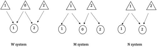
Figure 1 shows three ATO systems that are common in the literature. The W system has two products, and three components, one of which is used by both products. Each product is assembled from one unit of the common component and one unit of a product-specific component. With a slight deviation from the aforementioned notation, the common component is referred to as component 0. The M system uses two components to build three products. Products 1 and 2 use one unit of components 1 and 2, respectively. The third product, referred to as product 0 in a slight deviation from the aforementioned notation, uses one unit of both components. The N system is a special case of both the W and M systems. It has two products and two components. Product 0 uses one unit of both components 0 and 1 and Product 1 uses only one unit of component 0.

There are K distinct component lead times, $L_1<\cdots <L_K$. Define $L_0=0$ for notational convenience. Let n_k be the number of components with lead time L_k ($1\le k\le K$). Components are indexed according to an ascending order of their lead times. Let ${\overline{n}}_0=0$ and ${\overline{n}}_k={\sum }_{k^{\prime }\le k}{n}_{k^{\prime }}$ ($1\le k\le K$). Observe that ${\overline{n}}_K=n$. Thus, $\{{\overline{n}}_{k-1}+1,\dots ,{\overline{n}}_k\}$ are the indexes of components with lead times L_k ($1\le k\le K$). We associate each component j with an index k_j ($1\le k_j\le K$) such that $L_{k_j}$ is the lead time of component j ($1\le j\le n$). Without loss of generality, we arrange the rows of A in an order such that the submatrix A^k, composed of rows ${\overline{n}}_{k-1}+1,\mathrm{..},\text{ and }{\overline{n}}_k$ of A, specifies the use of components with lead time L_k ($1\le k\le K$).

Without loss of generality and for simplicity, we let the system start at a time when there is no inventory on-hand, no order in transit, and no backlog, and define that time to be $t=-L_K$. Demand arrives according to an integer vector valued compound Poisson process

where ${\mathcal{D}}_i(t)$ is the amount of demand for product i ($1\le i\le m$) that arrives during $[-L_K,t]$. The process $\{\mathcal{D}(t),t\ge 0\}$ is right continuous. The number of demand orders arriving during $[-L_K,t]$ ($t\ge -L_K$) is a Poisson process $\mathrm{\Lambda }=\{\mathrm{\Lambda }(t),t\ge -L_K\}$, and there is an associated independent and identically distributed (i.i.d.) sequence of random vectors that give order sizes. A generic element of this sequence is denoted by $\mathbf{S}=(S_1,S_2,\dots ,S_m)$, where S_i is the order size for product i. Although the elements of the sequence (the order size vectors) are independent, the components $(S_1,S_2,\dots ,S_m)$ within each vector can be dependent. Let denote the order arrival rate. Mean demand arriving within a unit of time is

The covariance matrix of $(\mathcal{D}(1)-\mathcal{D}(0))$ is denoted by $\mathbf{\Sigma }$, of which the diagonal elements, σ_ii, are variances of demand i ($1\le i\le m$) over a unit of time. Because the demand process is stationary, $\mathit{\mu }$ and $\mathbf{\Sigma }$ are also, respectively, the means and the covariance matrix of demands over $[t,t+1]$ ($t\ge -L_K$).

We assume that S_i has a finite moment of order 6, that is,

As will be evident from the proof of Theorem 4, we assume a finite moment of order 6 for a similar reason as that in Huh et al. (2009), which is to use the moment to bound the difference between two stochastic processes. (Beyond that, both the time horizon and stochastic processes involved are completely different between the two studies.)

2.2. Inventory Control Problem

Inventory control includes both replenishment and allocation decisions. For components with lead time L_k, the replenishment starts from time $-L_k$ and is defined by ${\mathcal{R}}^k(t)$ $(t\ge -L_k)$, an integer-valued vector process with n_k components. Each component of ${\mathcal{R}}^k(t),\hspace{0.17em}{\mathcal{R}}_j(t)$, represents the amount of component j ordered over the period $[-L_k,t]$ $({\overline{n}}_{k-1}+1\le j\le {\overline{n}}_k$). In this context, ${\mathcal{R}}^k(t)$ $(t\ge -L_k)$ should be nonnegative and nondecreasing, which we assume in the paper. Orders are placed at distinct points of time. Hence, we assume the process is right-continuous.

The allocation decision is specified via an m-dimensional, integer-valued process $\mathcal{Z}(t)$. Each component of $\mathcal{Z}(t),\hspace{0.17em}{\mathcal{Z}}_i(t)$ $(t\ge -L_K)$, represents the amount of demand for product i $(1\le i\le m)$ served over the period $[-L_K,t]$. We assume that $\mathcal{Z}(t)$ $(t\ge -L_K)$ is also nonnegative, nondecreasing, and right-continuous.

Both ${\mathcal{R}}^k(t)$ ($t\ge -L_k,\hspace{0.17em}1\le k\le K$) and $\mathcal{Z}(t)$ ($t\ge 0$) must be adapted to the filtration generated by the initial states of the system, as well as $\mathcal{D}(s)$ ($-L_K\le s\le t$), ${\mathcal{R}}^k(s)$ ($-L_k\le s<t,\hspace{0.17em}1\le k\le K$), and $\mathcal{Z}(s)$ ($-L_K\le s<t$), which means that policies under our consideration are nonanticipating.

For the inventory control to be feasible, at any point of time, the total amounts of demand served cannot exceed the amounts that have arrived. The amounts of components used cannot exceed the amounts that have been received. Because the replenishment of components with the lead time L_k starts at time $-L_k$ $(1\le k\le K)$, no unit is received and thus no demand can be served before time 0. In our model, these restrictions are formalized by the following assumptions:

Observe that by definition, ${\mathcal{R}}^k(t-L_k)$ $(t\ge 0,1\le k\le K)$ are the amounts of components ordered at least one lead time before time t.

For $t\ge 0$, the inventory level of components with the lead time L_k is

and the backlog level is

By (1), both ${\mathbf{I}}^k(t)$ $(1\le k\le K)$ and $\mathbf{B}(t)$ $(t\ge 0)$ are nonnegative. Also by (1) and our assumption about the replenishment starting times,

Let b_i be the cost of backlogging one unit of demand of product i ($1\le i\le m$) per unit of time. Let h_j be the cost of holding one unit of inventory of component j ($1\le j\le n$) per unit of time. We assume that h_j ($1\le j\le n$) and b_i ($1\le i\le m$) are strictly positive. Let

Then at each time t ($t\ge 0$), the system incurs the total inventory cost at the expected rate

The problem of inventory control is to develop integer-valued, nonnegative, nondecreasing, right-continuous, and nonanticipating vector processes ${\mathcal{R}}^k(t)$ ($t\ge -L_k,\hspace{0.17em}1\le k\le K$) and $\mathcal{Z}(t)$ ($t\ge -L_K$), subject to (1)–(3), to minimize the following long-run average expected total inventory cost:

2.3. Additional Variables, Processes, and Relationships

For the needs of our analysis, we introduce additional variables and processes and specify their relationships.

2.3.1. Variables and Processes.

The additional variables and processes, defined in terms of the more “primitive” processes introduced in Sections 2.1 and 2.2, are listed in Table 1 along with their definitions. For the convenience of the reader, Table 1 also includes the definitions of the inventory and backlog processes defined in Section 2.2. Further discussions of these quantities are as follows:

Table 1. Key Variables: Notation and Value

The first processes we introduce here denote increments of the processes $\mathcal{D}(t)$ $(t\ge -L_K),\hspace{0.17em}{\mathcal{R}}^k(t)$ $(t\ge -L_k,1\le k\le K)$, and $\mathcal{Z}(t)$ $(t\ge -L_K)$ over particular time intervals. Here $\mathbf{D}(t_1,t_2)$ denotes demand that arrives during the time interval $(t_1,t_2]$ ($-L_K\le t_1<t_2),\hspace{0.17em}{\mathbf{D}}^k(t)$ are special cases of $\mathbf{D}(t_1,t_2)$ with $t_1=t-L_k$ and $t_2=t-L_{k-1}$ $(t\ge -L_K+L_k,\hspace{0.17em}1\le k\le K$), and

We also use $\overline{\mathbf{D}}(t)$ as a shorthand of ${\overline{\mathbf{D}}}^1(t)$ $(t\ge 0)$. (Recall that $L_0=0$.) We also introduce some random vectors. Let ${\mathbf{D}}^k$ and ${\overline{\mathbf{D}}}^k$ be random vectors that follow the same distributions of ${\mathbf{D}}^k(t)$ and ${\overline{\mathbf{D}}}^k(t),\hspace{0.17em}1\le k\le K,\hspace{0.17em}t\ge 0$, respectively. Let $\overline{\mathbf{D}}$ be a random vector that follows the same distribution of $\overline{\mathbf{D}}(t)$. We also define

which follows the same distribution of $\mathbf{D}(t-L_k,t)$ $(t\ge -L_K+L_k,1\le k\le K)$. By stationarity of $\mathcal{D}(t)$, these distributions do not depend on t. Recall that we assumed that the demand process is right continuous. We let $\mathbf{d}(t)$ denote the demand that arrives at time $t,t\ge -L_K$ (if any).

Similarly, ${\mathbf{R}}^k(t)$ $(1\le k\le K)$ denotes the amounts of components ordered over the previous lead time, or for t < 0, since the beginning of the replenishment process. Each component of ${\mathbf{R}}^k(t),\hspace{0.17em}{R}_j(t)$ $(t\ge -L_k,{\overline{n}}_{k-1}+1\le j\le {\overline{n}}_k)$, represents the amount of component j that is in transit: ordered from the supplier but not yet arrived. The amounts of demand served over the interval $(t_1,t_2]$ is denoted by $\mathbf{Z}(t_1,t_2)$ $(-L_K\le t_1<t_2)$.

Next we introduce two additional processes: inventory position $\mathbf{I}{\mathbf{P}}^k(t)$ and component balance ${\mathbf{Q}}^k(t)$ $(t\ge -L_k,\hspace{0.17em}1\le k\le K)$. For $k=1,\dots ,K$, entries of $\mathbf{I}{\mathbf{P}}^k(t),\hspace{0.17em}I{P}_j(t)$ (${\overline{n}}_{k-1}+1\le j\le {\overline{n}}_k$), are the differences between the total amounts of components that have been ordered up to time t $(t\ge -L_k)$ and the total amounts needed to serve all demands that have arrived by that time. Entries of ${\mathbf{Q}}^k(t),\hspace{0.17em}{Q}_j(t)$ (${\overline{n}}_{k-1}+1\le j\le {\overline{n}}_k)$, are the differences between the amounts needed to serve demands and the total amounts that have been ordered and received.

Recall that the replenishment and allocation processes (which are the control processes) are assumed to be integer valued and right continuous. Thus, the controls are exercised at discrete time points. It is helpful to distinguish the values of certain processes immediately before these actions are taken. To this end, we let $\mathbf{I}{\mathbf{P}}^{k-}(t)$ $(1\le k\le K$) denote the inventory positions at time t $(t\ge -L_k)$ before placing any order at that time, and let ${\mathbf{B}}^{-}(t)$ $(t\ge -L_K)$ denote the backlog levels at time t $(t\ge -L_K$) before serving any demand at that time. In Table 1, $\mathbf{d}(t),\hspace{0.17em}\mathbf{I}{\mathbf{P}}^{k-}(t)$, and ${\mathbf{B}}^{-}(t)$ are defined using the left limits $\mathcal{D}(t^{-})$ $(t>-L_K),\hspace{0.17em}\mathbf{I}{\mathbf{P}}^k(t^{-})$ $(t>-L_k,\hspace{0.17em}1\le k\le K$), and $\mathbf{B}(t^{-})$ $(t>-L_K)$. These left limits exist because in (2) and (3), $\mathcal{D}(t)$ $(t\ge -L_K),\hspace{0.17em}{\mathcal{R}}^k(t)$ $(t\ge -L_k,\hspace{0.17em}1\le k\le K$), and $\mathcal{Z}(t)$ $(t\ge -L_K)$ are nondecreasing and right-continuous. One may also observe that by definition,

2.3.2. Relationships.

The key definitions (2) and (3), along with the definitions introduced in Section 2.3.1, allow us to obtain relationships that are useful in our analysis. Using (2) and (3), and the definitions of ${\mathbf{R}}^k(t)$ $(t\ge -L_k,\hspace{0.17em}1\le k\le K$) and $\mathbf{Z}(t)$ $(t\ge -L_K)$ in Table 1, changes of inventory and backlog levels over a lead time L_k can be determined by

Again using (2) and (3), along with definitions of ${\mathbf{R}}^k(t)$ and $\mathbf{I}{\mathbf{P}}^k(t)$ $(t\ge -L_k,\hspace{0.17em}1\le k\le K)$ in the table,

The second line corresponds to another definition of the inventory position in the literature: the total amount of the component in the system, including both on-hand inventory and orders in-transit, minus the amount needed to clear all existing backlog at that time.

Yet again using (2) and (3), along with the definition of ${\mathbf{Q}}^k(t)$ in the table, and then applying (6) and (7) to replace $\mathbf{B}(t)$ and ${\mathbf{I}}^k(t)$,

Observe that the negative of an entry of ${\mathbf{Q}}^k(t)$,

is commonly referred to as the net inventory of component j at time t $(t\ge 0)$: there is a shortage (surplus) of component j to clear existing backlogs at time t if $Q_j(t)>(<)0$.

2.3.3. Other Parameters.

Define

where element c_i of $\mathbf{c}$ represents the amount of inventory cost that can be removed from the system by serving one unit of demand i ($1\le i\le m$).

For convenience, we define additional variables to denote the smallest (nonzero) and largest components of A, $\mathbf{b},\hspace{0.17em}\mathbf{h}$, and $\mathbf{c}$ in Table 2 below.

3. Stochastic Program

As we outlined in Section 1, the first step of our analysis is to develop a multistage SP that provides a lower bound on the average inventory cost and sets the stage for developing inventory control policies to drive the cost toward that bound. To this end, we first present a relevant SP from the literature and discuss the intuition that underlies its formulation in Section 3.1. In Section 3.2, we transform this SP into an alternative SP that we use for policy development in Section 4.

3.1. Previous Result

For ATO systems formulated in the last section, theorem 1 in Reiman and Wang (2012) proves that

is a lower bound on $\mathcal{C}$, the long-run average cost defined in (5). Here $\overline{\mathbf{D}}$ is defined in Table 1, and ${\mathrm{\Phi }}^K(\mathit{\alpha })$ is the minimum objective value of the K + 1 stage stochastic program (SP): where ${\mathbf{D}}^k$ ($1\le k\le K$) are also defined in Table 1.

We now take the rest of this section to provide some intuition as to why the SP (10)–(11) yields a lower bound on the cost in the ATO inventory control problem. The basic idea is that the SP (10)–(11) is a relaxation of the actual ATO inventory control problem. The SP corresponds to myopically focusing on a single point of time, with no concern for the effect that any replenishment or allocation decision might have on costs at other points of time. Thus, in the presence of random demand, all decisions are put off until the last possible moment, allowing as much information about actual demand as possible to be used for the decisions.

To explain the SP in more detail, using (6) and (9), with k = K when substituting for $\mathbf{B}(t)$ and

when substituting for ${\mathbf{I}}^k(t)$ $(1\le k\le K)$, we can write the inventory cost at any time t $(t\ge 0)$ as

The cost at t depends only on states and processes over the period $[t-L_K,t]$. Comparing (10)–(11) with this expression for the cost, $\mathit{\alpha }$ corresponds to the initial backlog levels $\mathbf{B}(t-L_K)$ and $\mathbf{z}$ corresponds to $\mathbf{Z}(t-L_K,t)$, the amounts of demand served in the period $[t-L_K,t]$. For components with lead time L_k, ${\mathbf{I}}^k(t-L_k)+{\mathbf{R}}^k(t-L_k)+A^k\mathbf{Z}(t-L_K,t-L_k)$ includes the amounts in inventory at time $t-L_k$, the amounts that will arrive between $t-L_k$ and t from the pipeline, and the amounts used in the period $[t-L_K,t-L_k]$ $(1\le k\le K)$. Corresponding to the sum of these three quantities, ${\mathbf{y}}^k$ represents the total amounts of these components that can be used to serve demands in period $[t-L_K,t]$.

In (10)–(11), $\mathit{\alpha },\hspace{0.17em}\mathbf{z}$, and ${\mathbf{y}}^k$ $(1\le k\le K)$ are chosen to minimize the inventory cost with no constraint other than the ones that must be satisfied by the aforementioned counterparts of these variables in the ATO system. By (1)–(3), $\mathbf{B}(t)$ and ${\mathbf{I}}^k(t)$ $(1\le k\le K,\hspace{0.17em}t\ge 0$) are nonnegative, so using (6):

and

Correspondingly, in (11),

The information constraint in the SP is less obvious, as the sequential/recursive nature of its formulation both encodes and potentially obscures the information available when certain decisions are made. Although it is not needed in the definition of the SP, the information available when decisions are made in the SP can be described via a discrete filtration

where ${\mathcal{F}}_K=\{\varnothing ,\mathrm{\Omega }\}$ and ${\mathcal{F}}_k$ is the σ-field generated by $\{{\mathbf{D}}^K,\cdots {\mathbf{D}}^{k+1},{\mathbf{y}}^K,\cdots {\mathbf{y}}^{k+1}\}$ ($0\le k<K$). The set of optimal values of ${\mathbf{y}}^k$ is ${\mathcal{F}}_k$-measurable ($1\le k\le K$) and that of $\mathbf{z}$ is ${\mathcal{F}}_0$-measurable.

The filtration ${\mathcal{F}}_k$ $(0\le k\le K$) imitates the information available in the associated ATO system and is generated by both ${\mathbf{D}}^{k^{\prime }}$ and ${\mathbf{y}}^{k^{\prime }}$, corresponding, respectively, to histories of demand arrivals in periods $[t-L_{k^{\prime }},t-L_{k^{\prime }-1}]$ and decision making at times $t-L_k^{\prime }$ $(k<k^{\prime }\le K)$. In ATO systems, $t-L_k$ is the last moment of decision making that can affect the value of ${\mathbf{I}}^k(t-L_k)+{\mathbf{R}}^k(t-L_k)+A^k\mathbf{Z}(t-L_K,t-L_k)$, so letting ${\mathbf{y}}^k$ be adapted to ${\mathcal{F}}_k$ allows its value to be chosen with the maximum amount of information. This adaptedness is not explicitly enforced in the SP but is implicit in the recursive structure of the SP. When ${\mathrm{\Phi }}^k$ (which corresponds to stage $K+1-k$) is solved to obtain ${\mathbf{y}}^k$, the prior decisions ${\mathbf{y}}^K,\dots ,{\mathbf{y}}^{k+1}$ are all known, and $\mathbf{x}={\mathbf{D}}^K+\cdots +{\mathbf{D}}^{k+1}$ is known as well. Similarly, t is the last moment of decision making that can affect $\mathbf{Z}(t)$, so the choice of $\mathbf{z}$ is adapted to ${\mathcal{F}}_0$. It is not surprising that, with $\mathit{\alpha },\hspace{0.17em}\mathbf{z}$, and ${\mathbf{y}}^k$ $(1\le k\le K)$ chosen under the minimum constraints and maximum information, (10) is a lower bound on the expected cost of the ATO system at any given time t and hence a lower bound on its average cost $\mathcal{C}$.

3.2. New Development

The SP in (11) is not directly applicable to our analysis. As one may observe from (10)–(11), and as is shown in the proof of Theorem 2, $\mathbf{b}·\mathit{\alpha }+{\mathrm{\Phi }}^K(\mathit{\alpha })$ decreases in $\mathit{\alpha }$, and strictly so in many cases. Therefore, the lower bound $\underset{¯}{C}$ is not directly computable by solving (11) with any fixed $\mathit{\alpha }$. To reach the infimum in (10), $\mathit{\alpha }$, and thus ${\mathbf{y}}^k$ ($1\le k\le K$) and $\mathbf{z}$ often have to approach infinity, so one cannot make use of the optimal values of these decision variables for policy development.

To address this issue, we transform (11) into an alternative SP by replacing ${\mathbf{y}}^k$ in (11) with ${\mathbf{y}}^k-A^k\mathit{\alpha }$ $(1\le k\le K)$ and $\mathbf{z}$ with $\mathbf{z}-\mathit{\alpha }$ and, following (10), letting $\mathit{\alpha }$ approach infinity. The transformation removes $\mathit{\alpha }$ and the nonnegativity constraints in (11) and leads to

For any feasible solution $\mathit{\alpha },\hspace{0.17em}{\mathbf{y}}^k$ $(1\le k\le K)$, and $\mathbf{z}$ in (11), ${\mathbf{y}}^k-A^k\mathit{\alpha }$ $(1\le k\le K)$ and $\mathbf{z}-\mathit{\alpha }$ is a feasible solution to (13), so ${\phi }^K\le {\mathrm{\Phi }}^K(\mathit{\alpha })$ for all $\mathit{\alpha }$. Therefore, (13) can also be used to set a lower bound on the inventory cost of an ATO system, a result that we will formally present in Theorem 2. Here, we first prove that the optimal solution of (13) is bounded.

Theorem 1

(See Appendix A for Proof). For any given values of ${\mathbf{y}}^{k+1},\dots ,{\mathbf{y}}^K$, and $\mathbf{x}$, if ${\mathbf{y}}^{k*}=(y_{{\overline{n}}_{k-1}+1}^{*},\dots ,y_{{\overline{n}}_k}^{*})$ is an optimal solution to the SP in (13) at stage k, that is,

$${\mathbf{h}}^k·{\mathbf{y}}^{k*}+\mathbf{E}[{\phi }^{k-1}({\mathbf{y}}^{k*},{\mathbf{y}}^{k+1}\cdots ,{\mathbf{y}}^K,\mathbf{x}+{\mathbf{D}}^k)]$$

attains the value of ${\phi }^k({\mathbf{y}}^{k+1},\dots ,{\mathbf{y}}^K,\mathbf{x})$ $(k=K,\dots ,1)$, then

$$-\underset{¯}{\beta }(||\mathbf{x}|{|}_1+\mathbf{E}\left[||{\underset{¯}{\mathbf{D}}}^k|{|}_1\right]+{\displaystyle \sum _{l=k+1}^K|}|{\mathbf{y}}^l|{|}_1)\le y_j^{*}\le \overline{\beta }(||\mathbf{x}|{|}_1+\mathbf{E}\left[\left|\right|{\underset{¯}{\mathbf{D}}}^k|{|}_1\right]+1),{\overline{n}}_{k-1}<j\le {\overline{n}}_k,$$(14)

where ${\underset{¯}{\mathbf{D}}}^k$ $(1\le k\le K$) are random vectors defined in Table 1, and $\underset{¯}{\beta }$ and $\overline{\beta }$ are any constants that satify

$$\underset{¯}{\beta }\ge n\frac{{\overline{a}}^2}{\underset{¯}{a}}\frac{\overline{c}}{\underset{¯}{b}}\hspace{1em} \mathit{\text{and}}\hspace{1em}\overline{\beta }\ge \frac{\overline{a}}{\underset{¯}{a}}\frac{\overline{c}}{\underset{¯}{h}},$$

with constants on the right-hand side (RHS) of inequalities given in Table 2.

Table 2. Smallest and Largest Components of Relevant Vectors and Matrix

The formulation in (13) helps us to avoid the aforementioned issue with (10)–(11). By (14), the optimal solutions to the new SP are finite, so they can and will be used as parameters of our inventory policy. Moreover, instead of taking the infimum in (10), we can use the optimal objective value of (13), which is directly computable, to set the same lower bound on the cost objective.

Theorem 2

(See Appendix A for Proof). Let $\underset{¯}{C}$ be the lower bound defined in (10) and ${\phi }^K$ be the optimal objective value of the SP defined in (13). Then

$$\underset{¯}{C}={\phi }^K+\mathbf{b}·\mathbf{E}[\overline{\mathbf{D}}].$$(15)

For future analysis, we replace $\mathbf{z}$ with $\mathbf{B}=\mathbf{x}-\mathbf{z}$ in (13) to transform the last stage LP into

In ${\phi }_B^0({\mathbf{y}}^1,\dots ,{\mathbf{y}}^K,\mathbf{x}),\hspace{0.17em}\mathbf{B}$ represents the amounts of unserved demands and thus is analogous to $\mathbf{B}(t)$ ($t\ge -L_K$), backlog levels in the ATO system. Let ${\mathbf{y}}^{K*}$ be an optimal solution to ${\phi }^K,\hspace{0.17em}{\mathbf{y}}^{k*}$ be an optimal solution to ${\phi }^k({\mathbf{y}}^{k+1*},\dots ,{\mathbf{y}}^{K*},{\overline{\mathbf{D}}}^{k+1})$ ($1\le k<K$), ${\mathbf{z}}^{*}$ be an optimal solution to ${\phi }^0({\mathbf{y}}^{1*},\dots ,{\mathbf{y}}^{K*},\overline{\mathbf{D}})$, and ${\mathbf{B}}^{*}=\overline{\mathbf{D}}-{\mathbf{z}}^{*}$. Then by Theorem 2:

Because both components and products are measured in discrete units, (11) and (13) should be discrete optimization problems that can be difficult to solve exactly. For the purpose of setting a lower bound, if suffices to solve (13) without the integrality constraint, which is a continuous relaxation of the discrete problem. However, as will be shown in the next section, we will also use the SP to formulate inventory control policies, and for that purpose, the solutions need to be integer valued and satisfy certain uniqueness and continuity conditions. These issues will be addressed in Section 7.

4. Inventory Policy

Here, we will first describe the general idea that motivates our approach in Section 4.1, followed by developments of our replenishment and allocation policies in Sections 4.2 and 4.3, respectively. We will then make a few important observations in Section 4.4. A simple example that illustrates the application of our inventory policy, involving the N system, is given in Appendix B.

4.1. General Idea

To drive the average cost of the ATO system toward its SP-based lower bound in (13), we formulate inventory policies that mimic the optimal solution of this SP. As is commonly known and easily verifiable from (6)–(7), in an ATO system, the net inventory levels satisfy

The second equality allows us to rewrite the expected cost rate as the following function of inventory positions and backlog levels:

where $\mathbf{c}$ is defined in (9). Because $\overline{\mathbf{D}}\stackrel{d}{=}\mathbf{D}(t-L_K,t),\hspace{0.17em}\mathbf{E}[\overline{\mathbf{D}}]=\mathbf{E}[\mathbf{D}(t-L_K,t)]$. Thus, by a direct comparison of the cost rate in (18) with its lower bound in (17), at any time t $(t\ge 0)$,

Hence, the average inventory cost of an ATO system $(\mathcal{C})$ reaches its lower bound $(\underset{¯}{C})$ if (19)–(20) are both satisfied for all time. Based on this observation, we develop replenishment and allocation policies by using the SP solutions to set targets for inventory positions and backlog levels, keeping actual values “close” to these targets under feasibility constraints.

4.2. Replenishment Policy

4.2.1 Overview.

The RHS of (19) is determined in (13). For k = K, ${\mathbf{y}}^{K*}$ is constant, and for $k=K-1,\dots ,1,\hspace{0.17em}{\mathbf{y}}^{k*}$, $(k=K-1,\dots ,1)$ are determined recursively (going backward in k) on each sample path of $({\mathbf{D}}^K,\dots ,{\mathbf{D}}^{k+1})$ as values of ${\mathbf{y}}^k$ that minimize

where $\mathbf{x}$ denotes the value of ${\mathbf{D}}^K+\cdots +{\mathbf{D}}^{k+1}$ on that path.

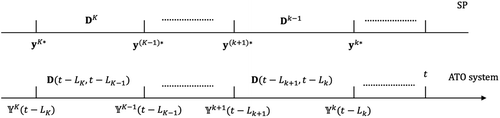
Our replenishment policy is built on processes ${\mathbb{Y}}^k(t)$ $(t\ge -L_k)$, with their distributions at each point of time mimicking those of ${\mathbf{y}}^{k*}$ $(1\le k\le K)$. Figure 2 shows a match of these two quantities in any period $[t-L_K,t]$ ($t\ge 0$). Let ${\mathbb{Y}}^K(t-L_K)={\mathbf{y}}^{K*}$, and determine ${\mathbb{Y}}^k(t-L_k)$ $(k=K-1,\cdots 1)$ recursively on each sample path of $\mathbf{D}(t-L_K,t-L_k)$ to minimize (21) with $\mathbf{x}=\mathbf{D}(t-L_K,t-L_k)$. Because $\mathbf{D}(t-L_k,t-L_{k-1})$ and ${\mathbf{D}}^k$ $(1\le k\le K)$ have the same distribution,

Motivated by (19), our policy uses ${\mathbb{Y}}^k(t-L_k)$ and $A^k\mathbf{D}(t-L_K,t-L_k)$ to set inventory position targets $\mathbb{I}{\mathbb{P}}^k(t)$ $(t\ge -L_k,1\le k\le K)$ and make ordering decision to move actual inventory positions $\mathbf{I}{\mathbf{P}}^k(t-L_k)$ $(t\ge -L_k,1\le k\le K)$ toward these targets.

Except for components with the longest lead time L_K, inventory position targets typically change over time. When a target rises above the actual inventory position, it is feasible to bring the latter position to its target immediately by ordering an appropriate amount of the component. When a target falls below the actual position, it is not feasible to close the gap immediately before the target is reduced and/or new demand arrives. Recognizing the latter restriction, our replenishment policy orders a component when and only when its inventory position is below the target, in the exact amount needed to eliminate the deficit.

4.2.2. Specific Policy Procedure.

For components with the longest lead time L_K, the inventory position target process starts from time $-L_K$ and is determined by

where ${\mathbb{Y}}^K$ is the value of ${\mathbf{y}}^K$ that minimizes

For components with lead time L_k $(k=K-1,\dots ,1)$, the target process starts from $-L_k$ and that its values are given by

where referring to (21) and the match shown in Figure 2, ${\mathbb{Y}}^k(t)$ is the value of ${\mathbf{y}}^k$ that minimizes

Starting from time $-L_k$, the actual inventory position of a component with lead time L_k is compared with its target. New replenishment is ordered to keep the actual inventory position at

where recognizing that inventory positions need to be integers, the ceiling function is applied to $\mathbb{I}{\mathbb{P}}^k(t)$. The “preorder” inventory position $\mathbf{I}{\mathbf{P}}^{k-}(t)$ $(t\ge -L_k,1\le k\le K)$ is defined in Table 1.

Although $\mathbb{I}{\mathbb{P}}^k(t)$ and $\mathbf{I}{\mathbf{P}}^k(t)$ $(t\ge -L_k,1\le k\le K)$ are both continuous-time processes, their values change only at discrete points of time, corresponding to new demand arriving at t, or a demand arrival at one of a particular set of previous times, as follows. For components with lead time L_K, as seen in (23), the procedure reduces to a constant base stock policy with ${\mathbb{Y}}^K$ as base stock levels. For components with lead time $L_{K-1},\hspace{0.17em}\mathbb{I}{\mathbb{P}}^{K-1}(t)$ needs to be updated only when there is a demand arrival at time $t+L_{K-1}-L_K$ or t, which changes the value of $\mathbf{D}(t+L_{K-1}-L_K,t)$, so (26) needs to be re-solved to update ${\mathbb{Y}}^{K-1}(t)$ $(t\ge -L_{K-1}$). Similarly, by induction on k in (26), for $k<K-1,\hspace{0.17em}\mathbb{I}{\mathbb{P}}^k(t)$ can change only when there is a demand arrival at time (i) t, which changes $\mathbf{D}(t+L_k-L_K,t)$, or (ii) $t+L_k-L_{k^{\prime }}$ ($k<k^{\prime }<K$) which might change ${\mathbb{Y}}^{k^{\prime }}(t+L_k-L_{k^{\prime }})$, or (iii) $t+L_k-L_K$, which changes both $\mathbf{D}(t+L_k-L_K,t)$ and ${\mathbb{Y}}^{k^{\prime }}(t+L_k-L_{k^{\prime }})$ ($k<k^{\prime }<K$). Moreover, (27) implies that only at these times can $\mathbf{I}{\mathbf{P}}^k(t)$ change: because $\mathbb{I}{\mathbb{P}}^k(t)$ can only change at these times, and as Table 1 shows, $\mathbf{I}{\mathbf{P}}^{k-}(t)$ can differ from $\mathbf{I}{\mathbf{P}}^k(t^{-})$ only when there is a demand arrival at time t $(t\ge -L_k,1\le k\le K$).

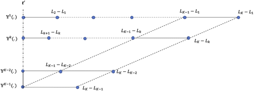
Although it may seem that an exact implementation of the previous idea would require looking back in time at every moment t, to see if there is any demand arrival at times $t+L_k-L_{k^{\prime }}$ $(k<k^{\prime }<K)$, to decide whether to update $\mathbb{I}{\mathbb{P}}^k(t)$ and place orders to reach new $\mathbf{I}{\mathbf{P}}^k(t)$ $(t\ge -L_k,1\le k\le K$), there is an equivalent simpler and more intuitive implementation, which allows demand arrivals to drive future updates. Specifically, when there is a demand arrival at time t, schedule updates of inventory position targets and corresponding ordering decisions at times $t,t+L_{k+1}-L_k,\dots ,t+L_K-L_k$ $(1\le k\le K-1)$.

Figure 3 illustrates the process. The vertical line represents a particular time $t^{\prime }$ when there is a demand arrival. Each horizontal line corresponds to a lead time. On the line corresponding to L_k, circles mark points of time when (26) needs to be re-solved to update ${\mathbb{Y}}^k(·)$ and $\mathbb{I}{\mathbb{P}}^k(·)$ $(1\le k<K$). The expression next to a circle shows the distance in time from time $t^{\prime }$ to the circle. Updates of ${\mathbb{Y}}^k(·)$ take place at times $t^{\prime }$ and $t^{\prime }+L_K-L_k$ as demand arrival at time $t^{\prime }$ changes $\mathbf{D}(t+L_k-L_K,t)$ in (26) when $t=t^{\prime }$ or $t=t^{\prime }+L_K-L_k$ $(1\le k<K)$. Moreover, as shown by two parallel dashed lines, updates of ${\mathbb{Y}}^{K-1}(·)$ at times $t^{\prime }$ and $t^{\prime }+L_K-L_{K-1}$ change values of ${\mathbb{Y}}^{K-1}(t+L_k-L_{K-1})$ in (26) when $t=t^{\prime }+L_{K-1}-L_k$ and $t=t^{\prime }+L_K-L_k$, so ${\mathbb{Y}}^k(·)$ needs to be updated at the latter two times $(1\le k<K-1$). In general updates of ${\mathbb{Y}}^k(·)$ at times $t^{\prime }$ and $t^{\prime }+L_K-L_k$ trigger updates of ${\mathbb{Y}}^l(·)$ at times $t^{\prime }+L_k-L_l$ and $t^{\prime }+L_K-L_l$, respectively $(1\le l<k$).

The complete replenishment procedure is presented in Algorithm 1. The collection of times at which ${\mathbb{Y}}^k(·),\hspace{0.17em}\mathbb{I}{\mathbb{P}}^k(·)$ and $\mathbf{I}{\mathbf{P}}^k(·)$ possibly change is denoted by ${\mathrm{\Gamma }}^k(1\le k\le K)$. The ceiling function on $\mathbb{I}{\mathbb{P}}_j(t)$ in step 2(c) ensures that both $I{P}_j(t)$ and ${\mathcal{R}}_j(t)$ are integer-valued ($t\ge -L_{k_j},1\le j\le n$). In Steps 2(a) and 2(b), inventory position targets $\mathbb{I}{\mathbb{P}}^k(t)$ $(t\ge -L_k,1\le k\le K$) are updated repeatedly over time except for k = K, in which case $\mathbb{I}{\mathbb{P}}^K(t)$ are constants that are set once at time $-L_K$. It is easy to verify that ${\mathcal{R}}_j(t)$ $(t\ge -L_{k_j},1\le j\le n)$ prescribed in Algorithm 1 satisfy the feasibility requirements defined in Section 2: integer-valued, nonnegative, nondecreasing, right-continuous, and nonanticipating.

It is worth pointing out that in ATO systems with a single product, this replenishment policy specializes to the one prescribed by Rosling (1989). In this special case, the latter policy is exactly optimal because all components are used according to fixed proportions, so one can always keep inventory positions at their targets (after some initial lapse for these positions to reach “coordinated levels”). In systems with identical lead times, our policy specializes to the one formulated in Reiman and Wang (2015), which uses base stock policies for replenishment and is asymptotically optimal in the large lead time regime.

Algorithm 1

(Replenishment Policy Procedure)

Initialization: for $k=1,\cdots K$, let

$${\mathrm{\Gamma }}^k=\{-L_k\},\hspace{1em}{\mathcal{R}}^k(-L_k^{-})=0,\hspace{1em}\text{ and}\hspace{1em}\mathbf{I}{\mathbf{P}}^k(-L_k)=-A^k\mathcal{D}(-L_k).$$

For $t\ge -L_K$:

1. if $\mathbf{d}(t)>0$, then for $k=1,\dots ,K$ such that $t\ge -L_k$, let

   $$\begin{array}{l}\mathbf{I}{\mathbf{P}}^{k-}(t)=\mathbf{I}{\mathbf{P}}^k(t^{-})-A^k\mathbf{d}(t).\hfill \\ \text{ and}\hspace{1em}\hspace{1em}\hspace{1em}\hspace{1em}{\mathrm{\Gamma }}^k={\mathrm{\Gamma }}^k\cup \{t,t+L_{k+1}-L_k,\dots ,t+L_K-L_k\}.\hfill \end{array}$$

2. for $k=1,\dots ,K$, if $t\in {\mathrm{\Gamma }}^k$, then:

   • (a) let ${\mathbb{Y}}^k(t)$ be the value of ${\mathbf{y}}^k$ that minimizes (26)

   • (b) as in (25), let

     $$\mathbb{I}{\mathrm{\mathbb{P}}}^k(t)={\mathbb{Y}}^k(t)-A^k\mathbf{D}(t+L_k-L_K,t).$$

   • (c) for each component j with lead time L_k, let

     $${\mathcal{R}}_j(t)={\mathcal{R}}_j(t^{-})+{\left(\lceil \mathbb{I}{\mathrm{\mathbb{P}}}_j(t)\rceil -I{P}_j^{-}(t)\right)}^{+},$$
         by ordering ${\left(\lceil \mathbb{I}{\mathrm{\mathbb{P}}}_j(t)\rceil -I{P}_j^{-}(t)\right)}^{+}$ units, changing its inventory position to
     $$I{P}_j(t)=I{P}_j^{-}(t)+{\mathcal{R}}_j(t)-{\mathcal{R}}_j(t^{-}).$$
     End of Algorithm 1

4.3. Allocation Policy

4.3.1. Overview.

On the RHS of (20), ${\mathbf{B}}^{*}$ is the optimal solution of the LP

which is defined on each sample path of $({\mathbf{D}}^K,\dots ,{\mathbf{D}}^1)$, with $\mathbf{x}$ denoting ${\mathbf{D}}^K+\cdots +{\mathbf{D}}^1$ and ${\mathbf{y}}^{k*}$ determined recursively by minimizing (21) for values of $({\mathbf{D}}^K,\dots ,{\mathbf{D}}^{k+1})$ ($1\le k\le K$) on the same path. In the corresponding ATO system, $\mathbf{D}(t-L_K,t)$ has the same distribution as ${\mathbf{D}}^K+\cdots +{\mathbf{D}}^1$ and ${\mathbb{Y}}^k(t-L_k)$ has the same distributions as ${\mathbf{y}}^{k*}$ $(t\ge 0,1\le k\le K)$. Hence, we can mimic ${\mathbf{B}}^{*}$ at time t $(t\ge 0)$ by letting ${\mathbb{B}}^{*}(t)$ be the value of $\mathbf{B}$ that minimizes (28) with $A^k\mathbf{x}-{\mathbf{y}}^{k*}$ replaced by

As a result, (20) holds for ${\mathbb{B}}^{*}(t)$, that is,

Although ${\mathbb{B}}^{*}(t)$ $(t\ge 0)$ gives the desired backlog levels for the inventory cost to reach its lower bound, it is determined by (see (25) and (29))

Comparing with ${\mathbf{Q}}^k(t)$ in Table 1, ${\mathbb{Q}}^k(t)$ differs from actual component balances by having inventory position targets $\mathbb{I}{\mathbb{P}}^k(t-L_k)$ in place of actual positions $\mathbf{I}{\mathbf{P}}^k(t-L_k)$ $(t\ge 0,1\le k\le K)$. Because our replenishment policy in general does not keep inventory positions at their targets, ${\mathbb{Q}}^k(t)$ does not always capture the exact state of component availability in the system. Recognizing this discrepancy, we set the backlog target at $\mathbb{B}(t)$ $(t\ge 0)$, which, like ${\mathbb{B}}^{*}(t)$, is determined by minimizing (28), but using ${\mathbf{Q}}^k(t)$ instead of ${\mathbb{Q}}^k(t)$ to replace $A^k\mathbf{x}-{\mathbf{y}}^{k*}$ $(1\le k\le K)$. Although (20) may not hold for $\mathbb{B}(t)$ $(t\ge 0)$ at equality, our analysis shows that the difference is asymptotically negligible.

Actual backlog levels may exceed or fall below their targets. It is generally infeasible to keep all backlog levels at their targets: a below-target backlog level cannot be raised immediately to the target if there is no new demand arrival, and an above-target backlog level cannot be reduced if a required component is not available. Naturally, we prescribe an allocation policy that uses all available components to reduce backlogs that are above their targets and never serves a demand when its backlog level is at or below the target.

Algorithm 2

(Allocation Policy Procedure)

Initialization: let

$$\mathcal{Z}(t)=0\hspace{1em}\text{ for all }t<0\hspace{1em}(\text{so }\mathbf{B}(0^{-})=\mathcal{D}(0^{-})).$$

For $t\ge 0$,

 if t = 0 or $Q_j(t)-Q_j(t^{-})\ne 0$ for some $j=1,\dots ,n$, then

•  1 .let $\mathbb{B}(t)$ be the value of $\mathbf{x}$ that minimizes:

  $$\left\{\mathbf{c}\mathbf{x}|\mathbf{x}\ge 0,A^k\mathbf{x}\ge {\mathbf{Q}}^k(t),1\le k\le K\right\}.$$(31)

•  2. let

  $$\mathcal{Z}(t)=\mathcal{D}(t)-\mathbf{B}(t),$$(32)
  where $\mathbf{B}(t)$ must be integer-valued and its choice satisfies:

  • (a) for all $i=1,\dots ,m$,

    $${\left[\lfloor B_i(t)-{\mathbb{B}}_i(t)\rfloor \right]}^{+}\wedge \underset{1\le j\le n}{\min }\{{(I_j(t)-a_{ji}+1)}^{+}\}=0,$$(33)
          and
    $$B_i^{-}(t)\wedge {\mathbb{B}}_i(t)\le B_i(t)\le B_i^{-}(t),$$(34)
          where
    $$B_i^{-}(t)=B_i(t^{-})+d_i(t),$$(35)
          and by definition (8),
    $$I_j(t)={\displaystyle \sum _{i^{\prime }=1}^m{a}_{j{i}^{\prime }}}{B}_{i^{\prime }}(t)-Q_j(t).$$

  • (b) for all $j=1,\dots ,n$,

    $${\displaystyle \sum _{i=1}^m{a}_{ji}}{B}_i(t)\ge Q_j(t).$$(36)
    End of Algorithm 2

4.3.2. Specific Policy Procedures.

Algorithm 2 prescribes the specific policy procedure that implements the previous idea on component allocation.

To explain, the allocation decision starts at time 0 when the first batches of replenishment orders arrive. Before that time, backlogs simply accumulate as new demands arrive. After that time, new allocations are triggered by changes of $Q_j(t)$ ($t\ge 0,\hspace{0.17em}1\le j\le n)$, the balance of some components. (This occurs as demands and replenishments arrive.) As Table 1 shows, ${\mathbf{Q}}^k(t)$ is the difference between the accumulated demand and supply, $A^k\mathcal{D}(t)-{\mathcal{R}}^k(t-L_k)$ $(t\ge 0,1\le k\le K)$. The former is a compound Poisson process and the latter is a pure jump process under the replenishment policy executed by Algorithm 1. Thus, allocation actions are taken at discrete points of time, which include using (31) to set backlog targets and serving demand under conditions (32)–(36). Of the latter conditions, (32) and (35) simply repeat definitions of ${\mathbf{B}}^{-}(t)$ and $\mathbf{B}(t)$ in Table 1. Distinct features of the policy are characterized by (33), (34), and (36).

• In (33), $B_i(t)$ is specified as an integer, ${\mathbb{B}}_i(t)$ is real number, and the floor function is applied to eliminate the rounding error in their difference. The equation defines the key feature of the policy: a backlog level can exceed its target (within the rounding error) only when the system runs out of a needed component to serve the demand, that is, when

  $$a_{ji}>{\displaystyle \sum _{i^{\prime }=1}^m{a}_{j{i}^{\prime }}}{B}_{i^{\prime }}(t)-Q_j(t)=I_j(t)\hspace{1em}\text{ for some }j(1\le j\le n).$$

• The left inequality of (34) requires that the backlog level of a demand ($B_i(t)$) should be kept at its existing level ($B_i^{-}(t))$ if the latter level does not exceed its target (${\mathbb{B}}_i(t)$).

• The right inequality of (34) encodes that serving a demand can only reduces its backlog level.

• Referring to (8), (36) is equivalent to

  $$I_j(t)\ge 0,\hspace{1em}1\le j\le n,$$
  that is, demands cannot be served with a nonexisting component.

In prescribing this procedure, we have omitted specific processes for determining $\mathbf{B}(t)$ $(t\ge 0)$ to satisfy (33), (34), and (36) because there can be many different ones. For instance, one can select all backlogs that exceed their targets and use available components to reduce them one at a time according to a particular order. Each backlog is reduced to the point where (33) applies, that is, either the backlog reaches the target or there are not enough components to bring it down further. This process obviously also satisfies (34) and (36). We can formulate many other processes by, for instance, changing the order by which backlogs are processed or not following a fixed order at all. Therefore, Algorithm 2 defines not a single policy but a family of eligible policies. Such policies always exist, for example, the one that follows the process we just described.

To show that this family of eligible policies satisfy requirements for feasible policies defined in Section 2: Once $\mathbf{B}(t)$ $(t\ge 0)$ is determined, the original allocation process $\mathcal{Z}(t)$ $(t\ge 0)$ is fully specified by (32). By (32) and (35), we can write

and use the right inequality of (34) to show that $\mathcal{Z}(t)$ $(t\ge 0)$ is nondecreasing, and also nonnegative as $\mathcal{Z}(t)=0$ for t < 0. Because the value of $\mathcal{Z}(t)$ $(t\ge 0)$ changes only at discrete points of time, the process is right-continuous. Apply the definition of ${\mathbf{Q}}^k(t)$ in Table 1, its alternative expression in (8), and use (32) to write from which it is easy to see that $\mathcal{Z}(t)$ $(t\ge 0)$ satisfies all conditions in (1).

From the first expression of ${\mathbf{Q}}^k(t)$ $(1\le k\le K,t\ge 0)$ in (8) and the constraints in the LP (31),

Therefore, for any given product i $(1\le i\le m)$,

Apply the inequality to (33) leads to the following important property of our allocation policy:

For any $i=1,\dots ,m$, if $B_i(t)-{\mathbb{B}}_i(t)\ge 1$, then

See Table 2 for definitions of $\overline{a}$ and $\underset{¯}{a}$.

By this property, our policy does not allow backlog of any product i to exceed its target by more than a rounding error when no backlog is below its target (i.e., ${\mathbb{B}}_{i^{\prime }}(t)\le B_{i^{\prime }}(t)$ for all $i^{\prime }\ne i$). A similar observation was made in Reiman and Wang (2015) for developing asymptotically optimal policies to manage ATO systems with identical lead times. Likewise, we will use this fact in Section 6.2.2.

4.4. Further Comments

Algorithms 1 and 2 show that our policies can be fully implemented by controlling inventory positions via (27) and choosing backlog levels that satisfy (33), (34), and (36). For brevity, from now on, we will only use the latter variables to characterize our policies, instead of invoking the original replenishment process ${\mathcal{R}}^k(t)$ $(t\ge -L_k,1\le k\le K)$ and allocation process $\mathcal{Z}(t)$ $(t\ge -L_K)$.

The procedures in these tables implicitly assume that there is no ambiguity about ${\mathbb{Y}}^k(t)$ $(t\ge -L_k,1\le k\le K)$ and $\mathbb{B}(t)$ $(t\ge 0)$, which is true if the related SPs for choosing these values all have unique optimal solutions. In Section 7, we will discuss how to perturb these SPs to satisfy the uniqueness condition without compromising asymptotic optimality.

5. Asymptotic Optimality

The rest of the paper will focus on performance evaluation, especially asymptotic optimality, of our policy, and this section provides a critical lead into this analysis. We first set up the asymptotic regime in Section 5.1. We then define the asymptotic optimality criteria in Section 5.2, followed by the development of a key theorem in Section 5.3 (Theorem 3) that specifies sufficient conditions for meeting these criteria.

5.1. Large Lead Time Asymptotic Regime

We introduce a family of systems indexed by L. In the L^th system, $L_k^{(L)}$ is the lead time of components ${\overline{n}}_{k-1}+1,\dots ,{\overline{n}}_k$ ($1\le k\le K$). The longest lead time $L_K^{(L)}=L$. We define the large lead time asymptotic regime by letting the longest lead time $L\to \infty$.

For convenience, define $L_0^{(L)}=0$. Let

We impose no assumptions on other lead times except that for all L,

5.1.1. Demand Process.

The L^th system is empty at time –L when the demand process ${\mathcal{D}}^{(L)}(t)$ ($t\ge -L$) starts. This process is the same as $\mathcal{D}(t)$ $(t\ge -L_K)$ in Section 2 except for the starting time. Similar to definitions of $\mathbf{D}(t_1,t_2)$ and $\mathbf{d}(t)$ in Table 1, let ${\mathbf{D}}^{(L)}(t_1,t_2)$ be the increment of ${\mathcal{D}}^{(L)}(t)$ over $(t_1,t_2]$ $(-L\le t_1<t_2)$, with $\mathit{\mu }$ and $\mathbf{\Sigma }$ denoting the mean and covariance matrix of ${\mathbf{D}}^{(L)}(t,t+1)$, and ${\mathbf{d}}^{(L)}(t)$ be the instantaneous change of ${\mathcal{D}}^{(L)}(t)$ at t $(t\ge -L)$. Define

Let ${\mathbf{D}}^{k(L)}$ be a random vector with the same distribution as ${\mathbf{D}}^{(L)}(0,L_k^{(L)}-L_{k-1}^{(L)})$ $(1\le k\le K)$. Then

has the same distribution as ${\widehat{\mathbf{D}}}^{(L)}(t-{\widehat{L}}_k^{(L)},t-{\widehat{L}}_{k-1}^{(L)})$ $(t\ge -1,1\le k\le K)$.

5.1.2. Replenishment and Inventory.

In the L^th system, replenishments of components with lead time $L_k^{(L)}$ start at time $-L_k^{(L)}$ ($1\le k\le K$). Following the policy description in Section 4.2, the inventory position targets are

where ${\mathbb{Y}}^{K(L)}(t)$ is a constant vector (and thus will be denoted by ${\mathbb{Y}}^{K(L)}$) that minimizes and ${\mathbb{Y}}^{k(L)}(t)$ $(1\le k<K)$ minimizes on the sample path of with $\mathbf{x}$ denoting the value of ${\mathbf{D}}^{(L)}(t+L_k^{(L)}-L,t)$ on that path.

Let $\mathbf{I}{\mathbf{P}}^{k(L)}(t)$ $(t\ge 0,1\le k\le K)$ be the actual inventory position in the L^th system. Under the aforementioned replenishment policy, for $k=1,\dots ,K$:

where the operator $\vee$ is applied componentwise. Component balances under the targeted and actual inventory positions are, respectively,

For $k=1,\dots ,K$, let

5.1.3. Allocation and Backlog.

Referring to our allocation policy in Algorithm 2, denote backlog targets $\mathbb{B}(t)$ in the L^th system by ${\mathbb{B}}^{(L)}(t)$ ($t\ge 0$). Denote backlog levels ${\mathbf{B}}^{-}(t)$ and $\mathbf{B}(t)$ by ${\mathbf{B}}^{(L)-}(t)$ and ${\mathbf{B}}^{(L)}(t)$ ($t\ge -L$), respectively. Hence, ${\mathbb{B}}^{(L)}(t)$ $(t\ge 0)$ is the optimal solution that minimizes

Corresponding to ${\mathbb{B}}^{*}(t)$ prescribed by (28)–(29), let ${\mathbb{B}}^{*(L)}(t)$ be the optimal solution to (43) with ${\mathbf{Q}}^{k(L)}(t)$ replaced by ${\mathbb{Q}}^{k(L)}(t)$ $(t\ge 0,1\le k\le K)$.

Define

Obviously, ${\widehat{\mathbb{B}}}^{*(L)}(t)$ and ${\widehat{\mathbb{B}}}^{(L)}(t)$ $(t\ge 0)$ are optimal solutions to (43) with ${\mathbf{Q}}^{k(L)}(t)$ replaced by ${\widehat{\mathbb{Q}}}^{k(L)}(t)$ and ${\widehat{\mathbf{Q}}}^{k(L)}(t)$ $(1\le k\le K,t\ge 0)$, respectively.

5.1.4. Inventory Cost.

In the L^th system, the long-run average expected inventory cost is

Using (18), the expected inventory cost rate can be written as

Define

Then

where the scaled inventory cost rate is defined to be and by applying (39), (42), and (44) to (45), ${\widehat{\mathcal{C}}}^{(L)}(t)$ can be written as

5.1.5. Summary of Definitions.

For future reference, we summarize the definitions made in this subsection for asymptotic analysis. Some vectors of random processes ${\mathbf{x}}^{(L)}(t)$ are centered and scaled componentwise by

where t varies in a proper range of time and the centering ${\overline{\mathbf{x}}}^{(L)}$ is proportional to L. Similar operations apply to increments of demand processes over some periods $(t_1,t_2]$ and demand vectors used in the lower bound SP. These definitions are given in Table 3.

Some other processes and variables are scaled componentwise (without any centering) by

and their definitions are summarized in Table 4.

5.2. Asymptotic Optimality Criterion

Applying Theorem 2 to the L^th system, the average inventory cost ${\mathcal{C}}^{(L)}$ has a lower bound ${\underset{¯}{C}}^{(L)}$, determined by the SP (13), using ${\mathbf{D}}^{k(L)}$ as inputs ${\mathbf{D}}^k$ $(1\le k\le K)$. Define

Let ${\mathcal{C}}_{\min }^{(L)}$ denote the infimum of the average inventory cost over all feasible policies. Because these values are bounded below by ${\underset{¯}{C}}^{(L)}$, this infimum exists. We show that our policy is asymptotically optimal in the traditional sense that

that is, the percentage difference between the cost and its minimum value converges to zero as the longest lead time becomes large.

Because ${\mathcal{C}}_{\min }^{(L)}\ge {\underset{¯}{C}}^{(L)}$, we have

Hence, we can prove (47) by showing that

and,

To show (48) is true, apply the SP (13) to the L^th system with following changes: let $i^{\prime }$ be a product with $a_{n{i}^{\prime }}>0$, where component n has the longest lead time L. Keep h_n and $b_{i^{\prime }}$ intact while resetting h_j = 0 $(j\ne n$) and b_i = 0 ($i\ne i^{\prime }$). The problem then becomes

where we use ${\overline{D}}_{i^{\prime }}^{(L)}$ to denote $D_{i^{\prime }}^{K(L)}$, which has the same distribution as $D_{i^{\prime }}^{(L)}(t-L,t)$ $(t\ge 0)$.

Let ${\phi }_n^{K(L)}$ be the optimal objective value of the above minimization problem. Obviously, ${\phi }_n^{K(L)}\le {\phi }^{K(L)}$, where ${\phi }^{K(L)}$ is the objective value of (13) specialized to the L^th system. Apply ${\phi }_n^{K(L)}$ and the new costs to (15) and compare the resulting value (denoted by $C_n^{(L)}$) with the lower bound and the minimum cost:

Furthermore, simple transformations of ${\phi }_n^{K(L)}$ shows that

is a Newsvendor model (unlike the standard formulation, here we allow y_n to be negative, but it is easy to see that $y_n<0$ is never optimal), so $C_n^{(L)}$ is proportional to the standard deviation of ${\overline{D}}_{i^{\prime }}^{(L)}$, which is on the order of $\sqrt{L}$, and (48) follows as a consequence.

Hence, to show (47) is satisfied, we only need to prove (49); that is, our policy is asymptotically optimal on the diffusion scale.

5.3. Sufficient Conditions for Asymptotic Optimality

The following theorem shows that (49) holds if inventory positions and backlog levels converge to their respective targets. Recall that these targets were set at levels at which the average inventory cost can attain its SP-based lower bound (see (19) and (20)). Although meeting these targets exactly is not possible in general, the theorem shows that meeting them on the diffusion scale, which we will prove to be feasible in the next section, is sufficient to guarantee asymptotic optimality.

Theorem 3.

In a family of systems indexed by their longest lead time L, if

$$\underset{L\to \infty }{\lim \sup }\left\{\underset{t\ge -{\widehat{L}}_{k_j}^{(L)}}{\sup }\mathbf{E}\left[\left|{\stackrel{⁁}{IP}}_j^{(L)}(t)-{\stackrel{⁁}{\mathbb{I}\mathbb{P}}}_j^{(L)}(t)\right|\right]\right\}=0,1\le j\le n,$$(50)

and

$$\underset{L\to \infty }{\lim \sup }\left\{\underset{t\ge 0}{\sup }\mathbf{E}\left[\left|{\widehat{B}}_i^{(L)}(t)-{\widehat{\mathbb{B}}}_i^{*(L)}(t)\right|\right]\right\}=0,1\le i\le m,$$(51)

then (49) holds; that is, our policy is asymptotically optimal on the diffusion scale, and (47) follows as a consequence.

Proof.

Following (17), in the L^th system,

$${\underset{¯}{C}}^{(L)}={\displaystyle \sum _{k=1}^K{\mathbf{h}}^k}·\left(\mathbf{E}\left[{\mathbf{y}}^{k*(L)}\right]-A^k\mathbf{E}\left[{\mathbf{D}}^{K(L)}\right]\right)+\mathbf{c}·\mathbf{E}\left[{\mathbf{B}}^{*(L)}\right],$$

where ${\mathbf{y}}^{k*(L)}$ $(1\le k\le K)$ is obtained from (13) and ${\mathbf{B}}^{*(L)}$ is obtained from (16).

Specializing (22) and (30) in our policy formulation to the L^th system:

$$\mathbf{E}[{\mathbf{y}}^{k*(L)}]=\mathbf{E}[{\mathbb{Y}}^{k(L)}(t-L_k^{(L)})],1\le k\le K\hspace{1em}\text{ and}\hspace{1em}\mathbf{E}[{\mathbf{B}}^{*(L)}]=\mathbf{E}[{\mathbb{B}}^{*(L)}(t)],\hspace{1em}t\ge 0.$$

Moreover, ${\mathbf{D}}^{K(L)}$ has the same distribution as ${\mathbf{D}}^{(L)}(t-L,t)$ $(t\ge 0)$ by definition. Thus,

$$\begin{array}{ll}{\underset{¯}{C}}^{(L)}\hfill & ={\displaystyle \sum _{k=1}^K{\mathbf{h}}^k}·(\mathbf{E}[{\mathbb{Y}}^{k(L)}(t-L_k^{(L)})]-A^k\mathbf{E}[{\mathbf{D}}^{(L)}(t-L,t)])+\mathbf{c}·\mathbf{E}[{\mathbb{B}}^{*(L)}(t)]\\ \hfill & ={\displaystyle \sum _{k=1}^K{\mathbf{h}}^k}·(\mathbf{E}[\mathbb{I}{\mathbb{P}}^{k(L)}(t-L_k^{(L)})]-A^k\mathbf{E}[{\mathbf{D}}^{(L)}(t-L_k^{(L)},t)])+\mathbf{c}·\mathbf{E}[{\mathbb{B}}^{*(L)}(t)],\hspace{1em}t\ge 0,\hfill \end{array}$$

where the second equality results from the determination of inventory position targets in (25).

By the definition of ${\widehat{\underset{¯}{C}}}^{(L)}$ and applying the second equality of the above equation:

$$\begin{array}{l}{\widehat{\underset{¯}{C}}}^{(L)}=\frac{\sum _{k=1}^K{\mathbf{h}}^k·(\mathbf{E}[\mathbb{I}{\mathbb{P}}^{k(L)}(Lt-L_k^{(L)})]-A^k\mathbf{E}[{\mathbf{D}}^{(L)}(Lt-L_k^{(L)},Lt)])+\mathbf{c}·\mathbf{E}[{\mathbb{B}}^{*(L)}(Lt)]}{\sqrt{L}}\hfill \\ ={\displaystyle \sum _{k=1}^K{\mathbf{h}}^k}·\left(\mathbf{E}\left[{\stackrel{⁁}{\mathbb{I}\mathbb{P}}}^{k(L)}(t-{\widehat{L}}_k^{(L)})\right]-A^k\mathbf{E}\left[{\widehat{\mathbf{D}}}^{(L)}(t-{\widehat{L}}_k^{(L)},t)\right]\right)+\mathbf{c}·\mathbf{E}\left[{\widehat{\mathbb{B}}}^{*(L)}(t)\right],\hspace{1em}t\ge 0.\hfill \end{array}$$

Comparing this with (46):

$$\begin{array}{l}{\widehat{\mathcal{C}}}^{(L)}-{\widehat{\underset{¯}{C}}}^{(L)}=\underset{T\to \infty }{\lim \sup }\frac{1}{T}{\displaystyle {\int }_0^T({\widehat{\mathcal{C}}}^{(L)}(t)-{\underset{¯}{\widehat{C}}}^{(L)})}dt=\underset{T\to \infty }{\lim \sup }\frac{1}{T}{\displaystyle {\int }_0^T{\displaystyle \sum _{k=1}^K{\mathbf{h}}^k}}·\left(\mathbf{E}\left[{\widehat{\mathbf{I}\mathbf{P}}}^{k(L)}(t-{\widehat{L}}_k^{(L)})\right]-\mathbf{E}\left[{\stackrel{⁁}{\mathbb{I}\mathbb{P}}}^{k(L)}(t-{\widehat{L}}_k^{(L)})\right]\right)dt+\underset{T\to \infty }{\lim \sup }\frac{1}{T}{\displaystyle {\int }_0^T\mathbf{c}}·\left(\mathbf{E}\left[{\widehat{\mathbf{B}}}^{(L)}(t)\right]-\mathbf{E}\left[{\widehat{\mathbb{B}}}^{*(L)}(t)\right]\right)dt.\hfill \end{array}$$(52)

The theorem follows immediately by applying (50) and (51) to (52). □

6. Proof of Sufficient Conditions

Continuing from Theorem 3, we prove in this section that (50)–(51) are satisfied under target stability conditions to be defined later. To put results obtained in this section in perspective, it was shown in Reiman and Wang (2015) that for systems with identical lead times only (51) was needed because asymptotic optimality can be achieved under a base-stock policy that keeps the inventory positions constant. The convergence (51) was shown in theorem 4 in Reiman and Wang (2015), whereas here it is shown in Corollary 2. The proof of (51) in Reiman and Wang (2015) does not carry over to this setting because it assumes the use of a base stock policy for replenishment.

Target Stability Conditions. Under our inventory policy, ${\mathbb{Y}}^k(t)$ $(t\ge -L_k,1\le k\le K)$, obtained by solving (26), ${\mathbb{B}}^{*}(t)$ ($t\ge 0$), obtained by solving (28)–(29), and $\mathbb{B}(t)$ $(t\ge 0)$, obtained by solving (31), have the following properties: there exists some constant κ, depending only on $\mathbf{h},\hspace{0.17em}\mathbf{b}$, and A, such that on each sample path of these processes,

• for all $t_2>t_1\ge -L_{k_j}$,

  $$|{\mathbb{Y}}_j(t_2)-{\mathbb{Y}}_j(t_1)|\le \kappa {\displaystyle \sum _{k>k_j}|}|\mathbf{D}(t_2-(L_k-L_{k_j}),t_2)-\mathbf{D}(t_1-(L_k-L_{k_j}),t_1)|{|}_1,\hspace{1em}1\le j\le n,$$(53)

• for all $t\ge 0$,

  $$|{\mathbb{B}}_i(t)-{\mathbb{B}}_i^{*}(t)|\le \kappa {\displaystyle \sum _{j=1}^n|}{Q}_j(t)-{\mathbb{Q}}_j(t)|,\hspace{1em}1\le i\le m,$$(54)
  and for all $t_2>t_1\ge 0$,
  $$|{\mathbb{B}}_i^{*}(t_2)-{\mathbb{B}}_i^{*}(t_1)|\le \kappa {\displaystyle \sum _{j=1}^n|}{\mathbb{Q}}_j(t_2)-{\mathbb{Q}}_j(t_1)|,\hspace{1em}1\le i\le m.$$(55)

We will develop an SP solution procedure in Section 7 to satisfy (53)–(55). Here in this section, we assume these conditions hold to prove (50) and (51).

Let us first give an informal explanation of the intuition of our proof. Under our replenishment policy, an inventory position can differ from its target only by exceeding it. When this happens, our policy will stop ordering the component, so its inventory position drops at the same rate as its demand arrival rate. The target may also change as new demand arrives. However, Condition (53) ensures that the latter change in the target is “slow” in comparison with demand arrivals, so the excess of inventory position over its target can be eliminated fast enough to satisfy (50). We then use a similar argument to show that under Conditions (54)–(55), (51) cannot be violated by having a backlog level falling below its target. To show that (51) can also not be violated by having a backlog level exceeding its target, we make use of the property of our allocation policy given in (37); that is, no backlog level will exceed its target when no other backlog level is below its target.

To reduce redundancy and improve generality, in Section 6.1, we define a general problem, referred to as the stochastic tracking model, based on common features of (50) and (51). We develop Theorem 4, which applies to the general model and contains (50) and (51) as special cases.

6.1. Stochastic Tracking Model

Consider a family of systems indexed by L > 0, where the L^th system is associated with the following parameters and processes:

• The process ${\mathcal{D}}^{(L)}(t)$ ($t\ge -L)$ is the same compound Poisson demand process defined in Section 5.1.1 for the L^th system, with the arrival rate $\underset{¯}{\lambda }$ and order sizes $\mathbf{S}$ apply to all systems. For the results of this section, it is important to recall that components of $\mathbf{S}$, S_i $(1\le i\le m)$, are assumed to have a finite moment of order 6. As in Section 5.1.1, the increment of ${\mathcal{D}}^{(L)}(t)$ over interval $(t_1,t_2]$ is denoted by ${\mathbf{D}}^{(L)}(t_1,t_2)$ $(-L\le t_1<t_2)$ and the jump of ${\mathcal{D}}^{(L)}(t)$ at time t is denoted by ${\mathbf{d}}^{(L)}(t)$ $(t\ge -L)$.

• The vector $\mathcal{A}$ is an m-dimensional vector of nonnegative integers. The value of the vector is the same for all systems and at least one of its elements is strictly positive.

• Each system is associated with a set of constants $s_l^{(L)}$ ($l\in \mathcal{K}$). Values of $s_l^{(L)}$ $(l\in \mathcal{K})$ differ between systems, but the index set $\mathcal{K}$, which is finite, remains the same for all systems. In the L^th system,

  $$0\le s_l^{(L)}\le L,\hspace{1em}(l\in \mathcal{K}).$$

• The process ${\mathcal{T}}^{(L)}(t)$ $(t\ge t_0^{(L)})$, which we refer to as the target process, is a pure jump process that starts at time $t_0^{(L)}$, where in the L^th system,

  $$-L+s_l^{(L)}\le t_0^{(L)}\le 0,\hspace{1em}\text{ and thus}\hspace{1em}{t}_0^{(L)}-s^{(L)}\ge -L,\hspace{1em}\text{ for all }\hspace{0.17em}\hspace{0.17em}l\in \mathcal{K}.$$

• The process ${\mathcal{W}}^{(L)}(t)$ $(t\ge t_0^{(L)})$, which we refer to as the tracking process, is another pure jump process that also starts at time $t_0^{(L)}$ from an initial level ${\mathcal{W}}_0^{(L)}$. The process is defined by

  $$\begin{array}{ll}{\mathcal{W}}^{(L)-}(t_0^{(L)})\hfill & ={\mathcal{W}}_0^{(L)},\hfill \\ {\mathcal{W}}^{(L)}(t)\hfill & ={\mathcal{W}}^{(L)-}(t)\vee {\mathcal{T}}^{(L)}(t)={\mathcal{T}}^{(L)}(t)+{({\mathcal{W}}^{(L)-}(t)-{\mathcal{T}}^{(L)}(t))}^{+}, t\ge t_0^{(L)},\hfill \\ {\mathcal{W}}^{(L)-}(t)\hfill & ={\mathcal{W}}^{(L)}(t^{-})-\mathcal{A}·{\mathbf{d}}^{(L)}(t),\hspace{1em}t>t_0^{(L)}.\hfill \end{array}$$(57)

For convenience, we denote the initial difference between the target and tracking processes by

Observe that the tracking process can instantly catch the target that rises higher than its level. When the target is lower, the gap can be closed after a sufficient amount of demand has arrived.

Let ${\widehat{\mathbf{D}}}^{(L)}(t_1,t_2)$ $(-1\le t_1<t_2)$ and ${\widehat{\mathbf{d}}}^{(L)}(t)$ $(t\ge -1)$ be defined the same as in (39). Let

Following the conditions imposed on $s_l^{(L)}$ and $t_0^{(L)}$ in their definitions,

Let

Finally, the definition of the model also requires the following asymptotic Lipschitz continuity condition on the target processes in this family of systems:

Asymptotic Lipschitz Condition. There exists some constant κ that applies to all systems, such that for all $t_0^{(L)}\le t_1<t_2$,

where ${\mathcal{E}}^{(L)}(t)$ ($t\ge t_0^{(L)}$) satisfies the following condition: let

Then

The main conclusion we draw from this model is in Theorem 4, which shows that as L increases, the tracking process converges to the target process on the diffusion scale.

Theorem 4.

Assume that S_i $(1\le i\le m)$ has a finite moment of order 6. If

$$\underset{L\to \infty }{\lim }\mathbf{E}[{\widehat{\mathcal{G}}}_0^{(L)}]=0,$$(61)

then

$$\underset{L\to \infty }{\lim }\mathbf{E}\left[\underset{t\ge {\widehat{t}}_0^{(L)}}{\sup }\left\{{\widehat{\mathcal{W}}}^{(L)}(t)-{\widehat{\mathcal{T}}}^{(L)}(t)\right\}\right]=0.$$(62)

Before proving the theorem, we provide some context and intuition for the result. The convergence in (62) is, in essence, an example of “state-space collapse,” a phenomenon that plays a critical role in the heavy traffic analysis of queueing systems and stochastic processing networks (Reiman 1984, Harrison and van Miegham 1997, Bramson 1998, Bell and Williams 2001, Atar et al. 2019). As noted previously, the tracking process ${\widehat{\mathcal{W}}}^{(L)}$ is able to instantly match the upward jumps of the target process but not the downward jumps. Under the scaling that we introduced, the family of processes ${\widehat{\mathbf{D}}}^{(L)}$ satisfies a functional central limit theorem (FCLT). This implies that ${\widehat{\mathbf{D}}}^{(L)}$ has “almost continuous” paths for large L. The assumed asymptotic Lipschitz continuity of ${\widehat{\mathcal{T}}}^{(L)}$ implies that it has almost continuous paths as well. When ${\widehat{\mathcal{W}}}^{(L)}(t)>{\widehat{\mathcal{T}}}^{(L)}(t)$, it is following total demand downward. This is uncentered demand, so that ${\widehat{\mathcal{W}}}^{(L)}$ is decreasing at a “rate” that is $O(\sqrt{L})$ when ${\widehat{\mathcal{W}}}^{(L)}(t)>{\widehat{\mathcal{T}}}^{(L)}(t)$. Thus, ${\widehat{\mathcal{W}}}^{(L)}$ never gets “far away” from ${\widehat{\mathcal{T}}}^{(L)}$, and the two-dimensional processes $({\widehat{\mathcal{T}}}^{(L)}(t),{\widehat{\mathcal{W}}}^{(L)}(t))$ “collapse” into a one-dimensional process with ${\widehat{\mathcal{T}}}^{(L)}(t)={\widehat{\mathcal{W}}}^{(L)}(t)$ in the limit. The proof of Theorem 4 makes this intuitive description rigorous.

As noted previously, ${\widehat{\mathbf{D}}}^{(L)}$ satisfies an FCLT. Interestingly, we never actually invoke this fact in our proofs. A key reason is that it would not be enough to obtain the result that we need. FCLTs involve convergence over a finite time interval. To prove asymptotic optimality under the long run average cost criterion that we use, we need uniform convergence over an infinite time interval, which does not follow from the FCLT.

The proof of Theorem 4 is built on the following four lemmas. The first two are restatements of two lemmas in Reiman and Wang (2015), and the next two are new. In all lemmas, order sizes S_i are assumed to have a finite moment of order $2+\delta$ ($\delta >0$), except for Lemma 3, which requires a stronger condition of having a finite moment of order 6.

Lemma 1

(Lemma 2 in Reiman and Wang 2015). For all $i=1,\dots ,m$,

$$\mathbf{E}\left[\underset{0\le \tau \le 1}{\sup }{\widehat{d}}_i^{(L)}(\tau )\right]\le 3{\underset{¯}{\lambda }}^{1/(2+\delta )}(1+{\eta }_i)L^{-\delta /\left(2\right(2+\delta \left)\right)},$$(63)

where $\underset{¯}{\lambda }$ is the demand arrival rate and ${\eta }_i≔\mathbf{E}[S_i^{2+\delta }]$ $(\delta >0)$.

Lemma 2

(Lemma 3 in Reiman and Wang 2015). For all $i=1,\dots ,m$,

$$\mathbf{E}\left[\underset{0\le \tau \le L^{-1/4}}{\sup }|{\widehat{D}}_i^{(L)}(0,\tau )|\right]\le (1+{\sigma }_{ii}^2)L^{-1/4}.$$(64)

This is where σ_ii is the variance of $D_i(0,1)$.

Let g be any strictly positive constant. Then for all $i=1,\dots ,m$,

$$\mathbf{E}\left[\underset{L^{-1/4}\le \tau \le 1}{\sup }{\left(\right|{\widehat{D}}_i^{(L)}(0,\tau )|-\sqrt{L}\tau g)}^{+}\right]\le \frac{{\sigma }_{ii}^2}{g}{L}^{-1/4}.$$(65)

Lemma 3

(See Appendix A for Proof). Assume that S_i has a finite moment of order 6 $(1\le i\le m)$. Let ν be any strictly positive constant. Then for all $i=1,\dots ,m$,

$$\underset{L\to \infty }{\lim }\mathbf{E}[\underset{t\ge 0}{\sup }{\left(|{\widehat{D}}_i^{(L)}(0,t)|-\sqrt{L}t\nu \right)}^{+}]=0.$$(66)

Lemma 4

(See Appendix A for Proof). Let ν be any strictly positive constant. Then for all $i=1,\dots ,m$,

$$\underset{L\to \infty }{\lim }\mathbf{E}\left[{\displaystyle \sum _{\tau =0}^{\infty }\underset{0\le t<1}{\sup }}{\left({\widehat{d}}_i^{(L)}(t)-\sqrt{L}\nu \tau \right)}^{+}\right]=0.$$(67)

The theorem is proved here by showing that there is uniform upper bound on the expected value at the left-hand side (LHS) on (62) and the bound converges to zero as L increases.

Proof of Theorem 4.

We prove (62) in the theorem by bounding ${({\widehat{\mathcal{W}}}^{(L)}(t)-{\widehat{\mathcal{T}}}^{(L)}(t))}^{+}$ and prove the bound converges uniformly to zero for all $t\ge {\widehat{t}}_0^{(L)}$. By definition,

$${\widehat{\mathcal{W}}}^{(L)}(t)\ge {\widehat{\mathcal{T}}}^{(L)}(t),\hspace{1em}t\ge {\widehat{t}}_0^{(L)},$$

so to bound ${({\widehat{\mathcal{W}}}^{(L)}(t)-{\widehat{\mathcal{T}}}^{(L)}(t))}^{+}$, we only need to consider the case where ${\widehat{\mathcal{W}}}^{(L)}(t)>{\widehat{\mathcal{T}}}^{(L)}(t)$, and for the latter case, only need to consider changes of ${\widehat{\mathcal{W}}}^{(L)}(t)-{\widehat{\mathcal{T}}}^{(L)}(t)$ since the last moment before t when ${\widehat{\mathcal{W}}}^{(L)}(·)$ jumps from ${\widehat{\mathcal{W}}}^{(L)}({\tau }^{-})={\widehat{\mathcal{T}}}^{(L)}({\tau }^{-})$ to ${\widehat{\mathcal{W}}}^{(L)}(\tau )>{\widehat{\mathcal{T}}}^{(L)}(\tau )$. That moment is defined by

$${\tilde{t}}^{(L)}=\underset{{\widehat{t}}_0^{(L)}\le \tau \le t}{\sup }\{\tau :{\widehat{\mathcal{W}}}^{(L)}(\tau )={\widehat{\mathcal{T}}}^{(L)}(\tau )\},$$

or if the set on the RHS is empty, let ${\tilde{t}}^{(L)}={\widehat{t}}_0^{(L)}$. Observe that, although not explicit in its notation, ${\tilde{t}}^{(L)}$ depends on t.

Observe that

$$|{\widehat{\mathcal{W}}}^{(L)}(t)-{\widehat{\mathcal{T}}}^{(L)}(t)|=({\widehat{\mathcal{W}}}^{(L)}(t)-{\widehat{\mathcal{T}}}^{(L)}(t))\mathbf{1}\{{\tilde{t}}^{(L)}={\widehat{t}}_0^{(L)}\}+({\widehat{\mathcal{W}}}^{(L)}(t)-{\widehat{\mathcal{T}}}^{(L)}(t))\mathbf{1}\{{\tilde{t}}^{(L)}>{\widehat{t}}_0^{(L)}\},$$(68)

so the proof of the theorem is reduced to proving

$$\underset{L\to \infty }{\lim }\mathbf{E}\left[\underset{t\ge {\widehat{t}}_0^{(L)}}{\sup }\left\{({\widehat{\mathcal{W}}}^{(L)}(t)-{\widehat{\mathcal{T}}}^{(L)}(t))\mathbf{1}\{{\tilde{t}}^{(L)}={\widehat{t}}_0^{(L)}\}\right\}\right]=0,$$(69)

$$\text{and }\underset{L\to \infty }{\lim }\mathbf{E}\left[\underset{t\ge {\widehat{t}}_0^{(L)}}{\sup }\left\{({\widehat{\mathcal{W}}}^{(L)}(t)-{\widehat{\mathcal{T}}}^{(L)}(t))\mathbf{1}\{{\tilde{t}}^{(L)}>{\widehat{t}}_0^{(L)}\}\right\}\right]=0.$$(70)

To prove (69), when ${\tilde{t}}^{(L)}={\widehat{t}}_0^{(L)},\hspace{0.17em}{\widehat{\mathcal{W}}}^{(L)}(\tau )>{\widehat{\mathcal{T}}}^{(L)}(\tau )$ for all $\tau \in [{\widehat{t}}_0^{(L)},t]$, so by (57),

$${\widehat{\mathcal{W}}}^{(L)}(t)-{\widehat{\mathcal{W}}}^{(L)}({\widehat{t}}_0^{(L)})=-\mathcal{A}·\frac{{\mathbf{D}}^{(L)}(L{\widehat{t}}_0^{(L)},Lt)}{\sqrt{L}}=-\mathcal{A}·({\widehat{\mathbf{D}}}^{(L)}({\widehat{t}}_0^{(L)},t)+\sqrt{L}\mathit{\mu }(t-{\widehat{t}}_0^{(L)})).$$

By applying the previous expression and Condition (59), for any time t $(t\ge {\widehat{t}}_0^{(L)})$,

$$\begin{array}{ll}{\widehat{\mathcal{W}}}^{(L)}(t)-{\widehat{\mathcal{T}}}^{(L)}(t)& =({\widehat{\mathcal{W}}}^{(L)}(t)-{\widehat{\mathcal{W}}}^{(L)}({\widehat{t}}_0^{(L)}))\hfill \\ & +{\widehat{\mathcal{G}}}_0^{(L)}-({\widehat{\mathcal{T}}}^{(L)}(t)-{\widehat{\mathcal{T}}}^{(L)}({\widehat{t}}_0^{(L)}))\\ & \le -\mathcal{A}·({\widehat{\mathbf{D}}}^{(L)}({\widehat{t}}_0^{(L)},t)+\sqrt{L}\mathit{\mu }(t-{\widehat{t}}_0^{(L)}))+{\widehat{\mathcal{G}}}_0^{(L)}\\ \hfill & +\kappa {\displaystyle \sum _{l\in \mathcal{K}}|}|{\widehat{\mathbf{D}}}^{(L)}(t-{\widehat{s}}_l^{(L)},t)-{\widehat{\mathbf{D}}}^{(L)}({\widehat{t}}_0^{(L)}-{\widehat{s}}_l^{(L)},{\widehat{t}}_0^{(L)})|{|}_1\hfill \\ & +|{\widehat{\mathcal{E}}}^{(L)}(t)|+|{\widehat{\mathcal{E}}}^{(L)}({\widehat{t}}_0^{(L)})|.\end{array}$$

Therefore, under Condition (61), (69) holds if

$$\begin{array}{l}\underset{L\to \infty }{\lim }\mathbf{E}\left[\underset{t\ge {\widehat{t}}_0^{(L)}}{\sup }\right\{-\mathcal{A}·[{\widehat{\mathbf{D}}}^{(L)}({\widehat{t}}_0^{(L)},t)+\sqrt{L}\mathit{\mu }(t-{\widehat{t}}_0^{(L)})]\hfill \\ +\kappa {\displaystyle \sum _{l\in \mathcal{K}}|}|{\widehat{\mathbf{D}}}^{(L)}(t-{\widehat{s}}_l^{(L)},t)-{\widehat{\mathbf{D}}}^{(L)}({\widehat{t}}_0^{(L)}-{\widehat{s}}_l^{(L)},{\widehat{t}}_0^{(L)})|{|}_1\left\}\right]=0,\hfill \end{array}$$(71)

which we prove next.

Let

$$\zeta =\frac{\mathcal{A}·\mathit{\mu }}{m(||\mathcal{A}|{|}_{\infty }+2\kappa |\mathcal{K}|)}>0\text{ and }\tilde{\kappa }=||\mathcal{A}|{|}_{\infty }+\kappa |\mathcal{K}|>0.$$

Then

$$\begin{array}{l}-\mathcal{A}·[{\widehat{\mathbf{D}}}^{(L)}({\widehat{t}}_0^{(L)},t)+\sqrt{L}\mathit{\mu }(t-{\widehat{t}}_0^{(L)})]+\kappa {\displaystyle \sum _{l\in \mathcal{K}}|}|{\widehat{\mathbf{D}}}^{(L)}(t-{\widehat{s}}_l^{(L)},t)-{\widehat{\mathbf{D}}}^{(L)}({\widehat{t}}_0^{(L)}-{\widehat{s}}_l^{(L)},{\widehat{t}}_0^{(L)})|{|}_1\le \Vert \mathcal{A}{\Vert }_{\infty }\Vert {\widehat{\mathbf{D}}}^{(L)}({\widehat{t}}_0^{(L)},t){\Vert }_1-\sqrt{L}\mathcal{A}·\mathit{\mu }(t-{\widehat{t}}_0^{(L)})\hfill \\ +\kappa {\displaystyle \sum _{l\in \mathcal{K}}(||{\widehat{\mathbf{D}}}^{(L)}(}{\widehat{t}}_0^{(L)},t)|{|}_1+\left|\right|{\widehat{\mathbf{D}}}^{(L)}({\widehat{t}}_0^{(L)}-{\widehat{s}}_l^{(L)},t-{\widehat{s}}_l^{(L)})|{|}_1)\hfill \\ \le \tilde{\kappa }{\displaystyle \sum _{i=1}^m(|{\widehat{D}}_i^{(L)}(}{\widehat{t}}_0^{(L)},t)|-\sqrt{L}\zeta (t-{\widehat{t}}_0^{(L)}){)}^{+}\hfill \\ +\kappa {\displaystyle \sum _{l\in \mathcal{K}}{\displaystyle \sum _{i=1}^m(|{\widehat{D}}_i^{(L)}(}}{\widehat{t}}_0^{(L)}-{\widehat{s}}_l^{(L)},t-{\widehat{s}}_l^{(L)})|-\sqrt{L}\zeta (t-{\widehat{t}}_0^{(L)}){)}^{+}.\hfill \end{array}$$(72)

Because ${\mathcal{D}}^{(L)}(t)$ ($t\ge -L$) is a stationary process,

$$|{\widehat{D}}_i^{(L)}({\widehat{t}}_0^{(L)},t)|\stackrel{d}{=}|{\widehat{D}}_i^{(L)}({\widehat{t}}_0^{(L)}-{\widehat{s}}_l^{(L)},t-{\widehat{s}}_l^{(L)})|\stackrel{d}{=}|{\widehat{D}}_i^{(L)}(0,t-{\widehat{t}}_0^{(L)})|,l\in \mathcal{K},1\le i\le m.$$(73)

Because ${\widehat{t}}_0^{(L)}\in [-1,0]$, for all $i=1,\dots ,m$,

$$\begin{array}{l}\underset{L\to \infty }{\lim }\mathbf{E}\left[\underset{t\ge {\widehat{t}}_0^{(L)}}{\sup }{(|{\widehat{D}}_i^{(L)}(0,t-{\widehat{t}}_0^{(L)})|-\sqrt{L}\zeta (t-{\widehat{t}}_0^{(L)}))}^{+}\right]\hfill \\ \le \underset{L\to \infty }{\lim }\mathbf{E}\left[\underset{t\ge t^{\prime }}{\sup }\underset{-1\le t^{\prime }\le 0}{\sup }{(|{\widehat{D}}_i^{(L)}(0,t-t^{\prime })|-\sqrt{L}\zeta (t-t^{\prime }))}^{+}\right]\hfill \\ =\underset{L\to \infty }{\lim }\mathbf{E}\left[\underset{t\ge 0}{\sup }{(|{\widehat{D}}_i^{(L)}(0,t)|-\sqrt{L}\zeta t)}^{+}\right]\hfill \\ =0(\text{Lemma }3),\hfill \end{array}$$(74)

and (71) follows directly from (72)–(74).

To prove (70), by the definition of ${\tilde{t}}^{(L)}$, in cases where ${\tilde{t}}^{(L)}>{\widehat{t}}_0^{(L)}$,

$${\widehat{\mathcal{W}}}^{(L)}({\tilde{t}}^{(L)-})={\widehat{\mathcal{T}}}^{(L)}({\tilde{t}}^{(L)-}),$$

and thus

$$\begin{array}{lll}{\widehat{\mathcal{W}}}^{(L)}(t)-{\widehat{\mathcal{T}}}^{(L)}(t)\hfill & =\hfill & {\widehat{\mathcal{W}}}^{(L)}(t)-{\widehat{\mathcal{T}}}^{(L)}(t)-[{\widehat{\mathcal{W}}}^{(L)}({\tilde{t}}^{(L)-})-{\widehat{\mathcal{T}}}^{(L)}({\tilde{t}}^{(L)-})]\hfill \\ \hfill & =\hfill & [{\widehat{\mathcal{W}}}^{(L)}(t)-{\widehat{\mathcal{W}}}^{(L)}({\tilde{t}}^{(L)})]+[{\widehat{\mathcal{W}}}^{(L)}({\tilde{t}}^{(L)})-{\widehat{\mathcal{W}}}^{(L)}({\tilde{t}}^{(L)-})]\hfill \\ \hfill & \hfill & +[{\widehat{\mathcal{T}}}^{(L)}({\tilde{t}}^{(L)-})-{\widehat{\mathcal{T}}}^{(L)}({\tilde{t}}^{(L)})]+[{\widehat{\mathcal{T}}}^{(L)}({\tilde{t}}^{(L)})-{\widehat{\mathcal{T}}}^{(L)}(t)].\hfill \end{array}$$(75)

Because ${\widehat{\mathcal{W}}}^{(L)}(\tau )>{\widehat{\mathcal{T}}}^{(L)}(\tau )$ for all $\tau \in ({\tilde{t}}^{(L)},t]$, by (57),

$$\begin{array}{ll}{\widehat{\mathcal{W}}}^{(L)}(t)-{\widehat{\mathcal{W}}}^{(L)}\left({\tilde{t}}^{(L)}\right)\hfill & =-\mathcal{A}·\left({\widehat{\mathbf{D}}}^{(L)}\right({\tilde{t}}^{(L)},t)+\sqrt{L}\mathit{\mu }(t-{\tilde{t}}^{(L)}\left)\right).\hfill \\ \hfill & \le \Vert \mathcal{A}{\Vert }_{\infty }{\displaystyle \sum _{i=1}^m|}{\widehat{D}}_i^{(L)}({\tilde{t}}^{(L)},t)|-\sqrt{L}(t-{\tilde{t}}^{(L)})\mathcal{A}·\mathit{\mu },\hfill \end{array}$$(76)

and

$${\widehat{\mathcal{W}}}^{(L)}({\tilde{t}}^{(L)})-{\widehat{\mathcal{W}}}^{(L)}({\tilde{t}}^{(L)-})=-\mathcal{A}·{\widehat{\mathbf{d}}}^{(L)}({\tilde{t}}^{(L)})\le 0.$$(77)

For the last two items in (75), by (59),

$$\begin{array}{l}\left|{\widehat{\mathcal{T}}}^{(L)}({\tilde{t}}^{(L)-})-{\widehat{\mathcal{T}}}^{(L)}({\tilde{t}}^{(L)})\right|\hfill \\ \le \kappa {\displaystyle \sum _{l\in \mathcal{K}}(||{\widehat{\mathbf{d}}}^{(L)}({\tilde{t}}^{(L)}-{\widehat{s}}_l^{(L)})|{|}_1+||{\widehat{\mathbf{d}}}^{(L)}({\tilde{t}}^{(L)})|{|}_1)}+{\widehat{\mathcal{E}}}^{(L)}({\tilde{t}}^{(L)-})+{\widehat{\mathcal{E}}}^{(L)}({\tilde{t}}^{(L)})\hfill \\ =\kappa {\displaystyle \sum _{i=1}^m{\displaystyle \sum _{l\in \mathcal{K}}(|{\widehat{d}}_i^{(L)}({\tilde{t}}^{(L)}-{\widehat{s}}_l^{(L)})|+|{\widehat{d}}_i^{(L)}({\tilde{t}}^{(L)})|)}}+{\widehat{\mathcal{E}}}^{(L)}({\tilde{t}}^{(L)-})+{\widehat{\mathcal{E}}}^{(L)}({\tilde{t}}^{(L)}),\hfill \end{array}$$(78)

and

$$\begin{array}{l}\left|{\widehat{\mathcal{T}}}^{(L)}\left({\tilde{t}}^{(L)}\right)-{\widehat{\mathcal{T}}}^{(L)}(t)\right|\hfill \\ \le \kappa {\displaystyle \sum _{l\in \mathcal{K}}|}\left|{\widehat{\mathbf{D}}}^{(L)}\right(t-{\widehat{s}}_l^{(L)},t)-{\widehat{\mathbf{D}}}^{(L)}({\tilde{t}}^{(L)}-{\widehat{s}}_l^{(L)},{\tilde{t}}^{(L)}\left)\right|{|}_1+{\widehat{\mathcal{E}}}^{(L)}\left({\tilde{t}}^{(L)}\right)+{\widehat{\mathcal{E}}}^{(L)}(t)\hfill \\ =\kappa {\displaystyle \sum _{l\in \mathcal{K}}|}\left|{\widehat{\mathbf{D}}}^{(L)}\right({\tilde{t}}^{(L)},t)-{\widehat{\mathbf{D}}}^{(L)}({\tilde{t}}^{(L)}-{\widehat{s}}_l^{(L)},t-{\widehat{s}}_l^{(L)}\left)\right|{|}_1+{\widehat{\mathcal{E}}}^{(L)}\left({\tilde{t}}^{(L)}\right)+{\widehat{\mathcal{E}}}^{(L)}(t)\hfill \\ \le \kappa {\displaystyle \sum _{i=1}^m{\displaystyle \sum _{l\in \mathcal{K}}\left(\left|{\widehat{D}}_i^{(L)}\right({\tilde{t}}^{(L)},t)|+|{\widehat{D}}_i^{(L)}({\tilde{t}}^{(L)}-{\widehat{s}}_l^{(L)},t-{\widehat{s}}_l^{(L)})|\right)}}+{\widehat{\mathcal{E}}}^{(L)}\left({\tilde{t}}^{(L)}\right)+{\widehat{\mathcal{E}}}^{(L)}(t).\hfill \end{array}$$(79)

Let

$$\nu =\frac{\mathcal{A}·\mathit{\mu }}{m(||\mathcal{A}|{|}_{\infty }+4\kappa |\mathcal{K}|)}.$$

By applying (76), (77), (78), and (79) to bound each item in the last expression of (75) and replacing $\mathcal{A}·\mathit{\mu }$ with $m(||\mathcal{A}|{|}_{\infty }+4\kappa |\mathcal{K}|)\nu$, we can prove that (70) holds under Condition (61) by showing that for all $i=1,\dots ,m$ and $l\in \mathcal{K}$,

$$\underset{L\to \infty }{\lim }\mathbf{E}\left[\underset{{\widehat{t}}_0^{(L)}\le t^{\prime }\le t<\infty }{\sup }{(|{\widehat{D}}_i^{(L)}(t^{\prime },t)|-\sqrt{L}(t-t^{\prime })\nu )}^{+}\right]=0,$$(80)

$$\underset{L\to \infty }{\lim }\mathbf{E}\left[\underset{{\widehat{t}}_0^{(L)}\le t^{\prime }\le t<\infty }{\sup }{\left(\left|{\widehat{D}}_i^{(L)}\right(t^{\prime }-{\widehat{s}}_l^{(L)},t-{\widehat{s}}_l^{(L)}\left)\right|-\sqrt{L}(t-t^{\prime })\nu \right)}^{+}\right]=0,$$(81)

$$\underset{L\to \infty }{\lim }\mathbf{E}\left[\underset{{\widehat{t}}_0^{(L)}\le t^{\prime }\le t<\infty }{\sup }{\left({\widehat{d}}_i^{(L)}(t^{\prime }-{\widehat{s}}_l^{(L)})-\sqrt{L}(t-t^{\prime })\nu \right)}^{+}\right]=0,$$(82)

$$\text{and }\underset{L\to \infty }{\lim }\mathbf{E}\left[\underset{{\widehat{t}}_0^{(L)}<t^{\prime }\le t<\infty }{\sup }{\left({\widehat{d}}_i^{(L)}\left(t^{\prime }\right)-\sqrt{L}(t-t^{\prime })\nu \right)}^{+}\right]=0.$$(83)

For each given i $(1\le i\le m)$ and l $(l\in \mathcal{K})$,

$$\begin{array}{lll}{\widehat{D}}_i^{(L)}(t^{\prime },t)\hfill & \stackrel{d}{=}\hfill & {\widehat{D}}_i^{(L)}(t^{\prime }-{\widehat{s}}_l^{(L)},t-{\widehat{s}}_l^{(L)})\stackrel{d}{=}{\widehat{D}}_i^{(L)}(0,t-t^{\prime }),\hspace{1em}{\widehat{t}}_0^{(L)}\le t^{\prime }\le t,\hfill \\ {\widehat{d}}_i^{(L)}(t-{\widehat{s}}_l^{(L)})\hfill & \stackrel{d}{=}\hfill & {\widehat{d}}_i^{(L)}(t^{\prime }),\hspace{1em}{t}^{\prime }\ge {\widehat{t}}_0^{(L)}.\hfill \end{array}$$

(Recall that $-1+{\widehat{s}}_l^{(L)}\le {\widehat{t}}_0^{(L)}$, so $t^{\prime }-{\widehat{s}}_l^{(L)}\ge -1$ in the previous expression). Therefore, (80) and (81) follow from a similar argument that proves (74): by the use of Lemma 3,

$$\underset{L\to \infty }{\lim }\mathbf{E}\left[\underset{{\widehat{t}}_0^{(L)}\le t^{\prime }\le t<\infty }{\sup }{\left(\left|{\widehat{D}}_i^{(L)}\right(t^{\prime },t\left)\right|-\sqrt{L}(t-t^{\prime })\nu \right)}^{+}\right]=\underset{L\to \infty }{\lim }\mathbf{E}\left[\underset{t\ge 0}{\sup }{\left(\left|{\widehat{D}}_i^{(L)}\right(0,t\left)\right|-\sqrt{L}t\nu \right)}^{+}\right]=0,$$

and

$$\begin{array}{l}\underset{L\to \infty }{\lim }\mathbf{E}\left[\underset{{\widehat{t}}_0^{(L)}\le t^{\prime }\le t<\infty }{\sup }{\left(\left|{\widehat{D}}_i^{(L)}\right(t^{\prime }-{\widehat{s}}_l^{(L)},t-{\widehat{s}}_l^{(L)}\left)\right|-\sqrt{L}(t-t^{\prime })\nu \right)}^{+}\right]\hfill \\ =\underset{L\to \infty }{\lim }\mathbf{E}\left[\underset{t\ge 0}{\sup }{\left(\left|{\widehat{D}}_i^{(L)}\right(0,t\left)\right|-\sqrt{L}t\nu \right)}^{+}\right]=0.\end{array}$$

To prove (82), because $-1+{\widehat{s}}_l^{(L)}\le {\widehat{t}}_0^{(L)}\le t^{\prime }\le t$ and the demand process is stationary,

$$\begin{array}{l}\mathbf{E}\left[\underset{{\widehat{t}}_0^{(L)}\le t^{\prime }\le t<\infty }{\sup }{\left({\widehat{d}}_i^{(L)}(t^{\prime }-{\widehat{s}}_l^{(L)})-\sqrt{L}(t-t^{\prime })\nu \right)}^{+}\right]\hfill \\ \le \mathbf{E}\left[\underset{-1\le t^{\prime }\le t<\infty }{\sup }{\left({\widehat{d}}_i^{(L)}\left(t^{\prime }\right)-\sqrt{L}(t-t^{\prime })\nu \right)}^{+}\right]\hfill \\ \le \mathbf{E}\left[\underset{t\ge 0}{\sup }\left({\displaystyle \sum _{\tau =0}^{\lfloor t\rfloor }{\left({\widehat{d}}_i^{(L)}\left(t^{\prime }\right)-\sqrt{L}\tau \nu \right)}^{+}}\mathbf{1}(t-\tau -1\le t^{\prime }\le t-\tau )+\underset{-1\le t^{\prime }\le 0}{\sup }{\widehat{d}}_i^{(L)}\left(t^{\prime }\right)\right)\right]\hfill \\ \le \mathbf{E}\left[{\displaystyle \sum _{\tau =0}^{\infty }\underset{0\le t^{\prime }\le 1}{\sup }}{\left({\widehat{d}}_i^{(L)}\left(t^{\prime }\right)-\sqrt{L}\tau \nu \right)}^{+}\right]+\mathbf{E}\left[\underset{-1\le t^{\prime }\le 0}{\sup }{\widehat{d}}_i^{(L)}\left(t^{\prime }\right)\right],\hfill \end{array}$$

and (82) follows from Lemmas 1 and 4. We then use the same argument to prove (83), and thus complete the proof of (70). □

6.2. Convergence to Targets

We again consider a family of ATO systems indexed by L, with ${\mathcal{D}}^{(L)}(t)$ $(t\ge -L)$ as the demand process in the L^th system. For each component and for each product, we specify other parameters in (56) to define an instance of the stochastic tracking model and prove (50) and (51) as corollaries of Theorem 4. In fact, the theorem shows convergence of $\mathbf{E}[\sup (·)]$ over an infinite time horizon, which is a stronger result than what is needed, which is the convergence of $\sup \mathbf{E}[(·)]$.

The proofs use the following lemma.

Lemma 5

(See Appendix A for Proof). Let ${\widehat{\mathbb{Y}}}_j^{(L)}(-{\widehat{L}}_{k_j}^{(L)})$ be defined in (42) with $t=-{\widehat{L}}_{k_j}^{(L)}$ $(1\le j\le n)$ and ν be any strictly positive constant. Then

$$\underset{L\to \infty }{\lim }\mathbf{E}[{(|{\widehat{\mathbb{Y}}}_j^{(L)}(-{\widehat{L}}_{k_j}^{(L)})|-\sqrt{L}\nu )}^{+}]=0,1\le j\le n.$$(84)

6.2.1. Proof of Condition (50).

For each component j $(1\le j\le n)$, define

To verify this is an instance of the stochastic tracking model, by our replenishment policy in Algorithm 1, $\lceil \mathbb{I}{\mathbb{P}}_j^{(L)}(t)\rceil$ ($t\ge 0$) is a pure jump process. Apply (25) to the L^th system,

Thus, under (53), the asymptotic Lipschitz condition (59)–(60) is satisfied with ${\mathcal{E}}^{(L)}(t)=1$.

By the definition of $I{P}_j^{-}(t)$ in Table 1 and referral to (27), in the L^th system,

which fits the definition of the tracking process ${\mathcal{W}}^{(L)}(t)$ $(t\ge t_0^{(L)})$. The initial value ${\mathcal{W}}_0^{(L)}$ is the inventory position of component j before the placement of the first order at time $-L_{k_j}^{(L)}$.

Corollary 1.

For all $j=1,\dots ,n$,

$$\underset{L\to \infty }{\lim }\mathbf{E}\left[\underset{t\ge -{\widehat{L}}_{k_j}^{(L)}}{\sup }\left|{\stackrel{⁁}{IP}}_j^{(L)}(t)-{\stackrel{⁁}{\mathbb{I}\mathbb{P}}}_j^{(L)}(t)\right|\right]=\underset{L\to \infty }{\lim }\mathbf{E}\left[\underset{t\ge -{\widehat{L}}_{k_j}^{(L)}}{\sup }\left|\frac{I{P}_j^{(L)}\left(Lt\right)-\lceil \mathbb{I}{\mathbb{P}}_j^{(L)}\left(Lt\right)\rceil }{\sqrt{L}}\right|\right]=0.$$(86)

Proof.

The first equality follows from definitions in (42) because the fractional value of $\mathbb{I}{\mathbb{P}}_j^{(L)}(Lt)$ can be ignored when $L\to \infty$. Theorem 4 shows that the second equality holds if

$$\underset{L\to \infty }{\lim }\mathbf{E}[{\widehat{\mathcal{G}}}_0^{(L)}]\triangleq \underset{L\to \infty }{\lim }\frac{{({\mathcal{W}}_0^{(L)}-{\mathcal{T}}^{(L)}(t_0^{(L)}))}^{+}}{\sqrt{L}}=0,$$

where by (85), for given j ($1\le j\le n$),

$${\widehat{\mathcal{G}}}_0^{(L)}={(\frac{-{\mathbf{A}}_j·{\mathbf{D}}^{(L)}(-L,-L_{k_j}^{(L)})-\lceil \mathbb{I}{\mathbb{P}}_j^{(L)}(-L_{k_j}^{(L)})\rceil }{\sqrt{L}})}^{+}.$$

Applying (25) to the L^th system,

$$\mathbb{I}{\mathbb{P}}_j^{(L)}(-L_{k_j}^{(L)})={\mathbb{Y}}_j^{(L)}(-L_{k_j}^{(L)})-{\mathbf{A}}_j·{\mathbf{D}}^{(L)}(-L,-L_{k_j}^{(L)}).$$

Therefore, by Lemma 5 with $\nu ={\mathbf{A}}_j·\mathit{\mu }$,

$$\underset{L\to \infty }{\lim }{\widehat{\mathcal{G}}}_0^{(L)}=\underset{L\to \infty }{\lim }\mathbf{E}\left[\frac{{\left(-{\mathbb{Y}}_j^{(L)}(-L_{k_j}^{(L)})\right)}^{+}}{\sqrt{L}}\right]\le \underset{L\to \infty }{\lim }\mathbf{E}\left[{\left(\left|{\widehat{\mathbb{Y}}}_j^{(L)}\right(-{\widehat{L}}_{k_j}^{(L)}\left)\right|-\sqrt{L}{\mathbf{A}}_j·\mathit{\mu }\right)}^{+}\right]=0.\hspace{1em}\square$$

6.2.2. Proof of Condition (51).

It is helpful to first review the processes that will be involved in the analysis. In the L^th system and for product i $(1\le i\le m$), ${\mathbb{B}}_i^{(L)}(t)$ $(t\ge 0)$ is the backlog target and ${\mathbb{B}}_i^{*(L)}(t)$ $(t\ge 0)$ is the ideal backlog level for reaching our SP-based lower bound. Both are determined by the LP in (43), using actual inventory positions and inventory position targets as their respective inputs. The backlog level under our allocation policy is $B_i^{(L)}(t)$ $(t\ge 0)$. To help with the analysis, we will define below an auxiliary process ${\underset{¯}{B}}_i^{(L)}(t)$ $(t\ge 0)$, which mimics $B_i^{(L)}(t)$ $(t\ge 0)$, except that it is not allowed to rise above the target ${\mathbb{B}}_i^{(L)}(t)$ $(t\ge 0)$.

For each product i $(1\le i\le m)$, we construct an instance of the stochastic tracking model by letting

where ${\underset{¯}{B}}_i^{(L)}(t)$ $(t\ge 0)$ is defined by

Here, we will show that $-{\mathbb{B}}_i^{(L)}(t)$ $(t\ge 0)$ is a target process, which, following the previous definition, also implies that $-{\underset{¯}{B}}_i^{(L)}(t)$ $(t\ge 0)$ is a tracking process.

When defining our allocation policy in Section 4.3.2, we have shown that ${\mathbb{B}}_i^{(L)}(t)$ ($t\ge 0$) is a pure jump process. To show that $-{\mathbb{B}}_i^{(L)}(t)$ $(t\ge 0)$ is asymptotically Lipschitz continuous, let

Then

which satisfies conditions (59)–(60) because

1. By applying (29) to (55), there exists some constant κ such that

   $$\begin{array}{l}|{\mathbb{B}}_i^{*(L)}(t_1)-{\mathbb{B}}_i^{*(L)}(t_2)|\le \kappa {\displaystyle \sum _{j=1}^n}(|{\mathbf{A}}_j{\mathbf{D}}^{(L)}(t_2-L,t_2)-{\mathbf{A}}_j{\mathbf{D}}^{(L)}(t_1-L,t_1)|\hfill \\ +|{\mathbb{Y}}_j^{(L)}(t_2-L_{k_j}^{(L)})-{\mathbb{Y}}_j^{(L)}(t_1-L_{k_j}^{(L)})|),\hfill \end{array}$$

   where under (53), there also exists some constant κ such that

   $$\begin{array}{ll}\hfill & |{\mathbb{Y}}_j^{(L)}(t_2-L_{k_j}^{(L)})-{\mathbb{Y}}_j^{(L)}(t_1-L_{k_j}^{(L)})|\hfill \\ \le \hfill & \kappa {\displaystyle \sum _{k>k_j}|}|{\mathbf{D}}^{(L)}(t_2-L_k^{(L)},t_2-L_{k_j}^{(L)})-{\mathbf{D}}^{(L)}(t_1-L_k^{(L)},t_1-L_{k_j}^{(L)})|{|}_1\hfill \\ \le \hfill & \kappa {\displaystyle \sum _{k>k_j}}(||{\mathbf{D}}^{(L)}(t_2-L_k^{(L)},t_2)-{\mathbf{D}}^{(L)}(t_1-L_k^{(L)},t_1)|{|}_1+||{\mathbf{D}}^{(L)}(t_2-L_{k_j}^{(L)},t_2)-{\mathbf{D}}^{(L)}(t_1-L_{k_j}^{(L)},t_1)|{|}_1).\hfill \end{array}$$

2. By (54), there exists some constant κ such that

   $$|{\mathcal{E}}^{(L)}(t)|\le \kappa {\displaystyle \sum _{j=1}^n|}{\mathbb{Q}}_j^{(L)}(t)-Q_j^{(L)}(t)|=\kappa {\displaystyle \sum _{j=1}^n|}I{P}_j^{(L)}(t-L_{k_j}^{(L)})-\mathbb{I}{\mathbb{P}}_j^{(L)}(t-L_{k_j}^{(L)})|,\hspace{1em}t\ge 0.$$

   Thus, (60) follows directly from Corollary 1.

Having shown that $(-{\mathbb{B}}_i^{(L)}(t),-{\underset{¯}{B}}_i^{(L)}(t))$ $(t\ge 0)$ is an instance of the target and tracking processes, we now can prove (51) as the following corollary to Theorem 4.

Corollary 2.

For $i=1,\dots ,m$, let

$${\underset{¯}{\widehat{B}}}_i^{(L)}(t)=\frac{{\underset{¯}{B}}_i^{(L)}(Lt)}{\sqrt{L}}.$$

Then,

$$\underset{L\to \infty }{\lim }\mathbf{E}[\underset{t\ge 0}{\sup }\left|{\widehat{\mathbb{B}}}_i^{(L)}(t)-{\underset{¯}{\widehat{B}}}_i^{(L)}(t)\right|]=0,$$(89)

which implies Condition (51).

Proof.

By Theorem 4, (89) holds if

$$\underset{L\to \infty }{\lim }\mathbf{E}[\left|{\widehat{\mathbb{B}}}_i^{(L)}(0)-{\underset{¯}{\widehat{B}}}_i^{(L)}(0)\right|]=0.$$(90)

To prove this initial condition, observe that

$${\mathbb{B}}_i^{(L)}(0)-{\underset{¯}{B}}_i^{(L)}(0)={\mathbb{B}}_i^{(L)}(0)-{\mathbb{B}}_i^{(L)}(0)\wedge B_i^{(L)-}(0)={({\mathbb{B}}_i^{(L)}(0)-B_i^{(L)-}(0))}^{+}={({\mathbb{B}}_i^{(L)}(0)-D_i^{(L)}(-L,0))}^{+}.$$

Because ${\mathbb{B}}_i^{(L)}(0)$ minimizes (31) with $\mathbf{Q}(t)={\mathbf{Q}}^{(L)}(0)$, there exists some constant κ, which depends only on matrix A, such that

$${\mathbb{B}}_i^{(L)}(0)\le \kappa {\displaystyle \sum _{j=1}^n{[Q_j^{(L)}(0)]}^{+}}=\kappa {\displaystyle \sum _{j=1}^n{[{\mathbf{A}}_j·{\mathbf{D}}^{(L)}(-L_{k_j}^{(L)},0)-I{P}_j^{(L)}(-L_{k_j}^{(L)})]}^{+}}.$$

Because $\mathbb{I}{\mathbb{P}}_j^{(L)}(-L_{k_j}^{(L)})\le I{P}_j^{(L)}(-L_{k_j}^{(L)})$ $(1\le j\le n)$ under our replenishment policy (see (27)),

$$\begin{array}{ll}{\mathbb{B}}_i^{(L)}(0)-D_i^{(L)}(-L,0)\hfill & \le \kappa {\displaystyle \sum _{j=1}^n{[{\mathbf{A}}_j·{\mathbf{D}}^{(L)}(-L_{k_j}^{(L)},0)-\mathbb{I}{\mathbb{P}}_j^{(L)}(-L_{k_j}^{(L)})]}^{+}}-D_i^{(L)}(-L,0)\hfill \\ \hfill & =\kappa {\displaystyle \sum _{j=1}^n{[{\mathbf{A}}_j·{\mathbf{D}}^{(L)}(-L,0)-{\mathbb{Y}}_j^{(L)}(-L_{k_j}^{(L)})]}^{+}}-D_i^{(L)}(-L,0).\hfill \end{array}$$

Let $\nu ={\mu }_i/(\kappa n(m\overline{a}+1)+1)$. By its definition, ${\underset{¯}{B}}_i^{(L)}(0)={\mathbb{B}}_i^{(L)}(0)\wedge D_i^{(L)}(-L,0)$. Therefore,

$$\begin{array}{l}\left|{\widehat{\mathbb{B}}}_i^{(L)}(0)-{\underset{¯}{\widehat{B}}}_i^{(L)}(0)\right|\hfill \\ \le \frac{1}{\sqrt{L}}{(\kappa {\displaystyle \sum _{j=1}^n{[{\mathbf{A}}_j·{\mathbf{D}}^{(L)}(-L,0)-{\mathbb{Y}}_j^{(L)}(-L_{k_j}^{(L)})]}^{+}}-D_i^{(L)}(-L,0))}^{+}\hfill \\ \le {(\kappa {\displaystyle \sum _{j=1}^n{\mathbf{A}}_j}·|{\widehat{\mathbf{D}}}^{(L)}(-1,0)|+\kappa {\displaystyle \sum _{j=1}^n|}{\widehat{\mathbb{Y}}}_j^{(L)}(-{\widehat{L}}_{k_j})|-\sqrt{L}{\mu }_i-{\widehat{D}}_i^{(L)}(-1,0))}^{+}\le n\kappa \overline{a}{\displaystyle \sum _{i^{\prime }=1}^m{(|{\widehat{D}}_{i^{\prime }}(-1,0)|-\sqrt{L}\nu )}^{+}}+\kappa {\displaystyle \sum _{j=1}^n{(|{\widehat{\mathbb{Y}}}_j^{(L)}(-{\widehat{L}}_{k_j})|-\sqrt{L}\nu )}^{+}}+{\left({\widehat{D}}_i^{(L)}(-1,0)-\sqrt{L}\nu \right)}^{+}.\hfill \end{array}$$

Because ${\mathcal{D}}^{(L)}(t)$ $(t\ge -L$) is stationary, Lemmas 3 and 5 imply (90), which proves (89).

To show that (89) implies (51),

$$|{\widehat{B}}_i^{(L)}(t)-{\widehat{\mathbb{B}}}_i^{*(L)}(t)|\le |{\widehat{B}}_i^{(L)}(t)-{\widehat{\mathbb{B}}}_i^{(L)}(t)|+|{\widehat{\mathbb{B}}}_i^{(L)}(t)-{\widehat{\mathbb{B}}}_i^{*(L)}(t)|.$$

By (88), the last term is simply ${\widehat{\mathcal{E}}}^{(L)}(t)$ that satisfies (60); thus, we only need to prove

$$\underset{L\to \infty }{\lim }\mathbf{E}\left[\underset{t\ge 0}{\sup }\left|{\widehat{B}}_i^{(L)}(t)-{\widehat{\mathbb{B}}}_i^{(L)}(t)\right|\right]=0.$$(91)

As is shown in (34), under our allocation policy,

$$B_i^{(L)}(t)\ge B_i^{(L)-}(t)\wedge {\mathbb{B}}_i^{(L)}(t)={\underset{¯}{B}}_i^{(L)}(t),\hspace{1em}\hspace{1em}t\ge 0,$$

and thus

$${\left({\widehat{\mathbb{B}}}_i^{(L)}(t)-{\widehat{B}}_i^{(L)}(t)\right)}^{+}\le {\left({\widehat{\mathbb{B}}}_i^{(L)}(t)-{\underset{¯}{\widehat{B}}}_i^{(L)}(t)\right)}^{+}=\left|{\widehat{\mathbb{B}}}_i^{(L)}(t)-{\underset{¯}{\widehat{B}}}_i^{(L)}(t)\right|,\hspace{1em}t\ge 0.$$

Moreover, because Property (37) applies when $B_i^{(L)}(t)-{\mathbb{B}}_i^{(L)}(t)\ge 1$, in all cases,

$${\widehat{B}}_i^{(L)}(t)-{\widehat{\mathbb{B}}}_i^{(L)}(t)\le \frac{1}{\sqrt{L}}+\frac{\overline{a}}{\underset{¯}{a}}{\displaystyle \sum _{i^{\prime }\ne i}{\left({\widehat{\mathbb{B}}}_{i^{\prime }}^{(L)}(t)-{\widehat{B}}_{i^{\prime }}^{(L)}(t)\right)}^{+}}\le \frac{1}{\sqrt{L}}+\frac{\overline{a}}{\underset{¯}{a}}{\displaystyle \sum _{i^{\prime }\ne i}\left|{\widehat{\mathbb{B}}}_{i^{\prime }}^{(L)}(t)-{\underset{¯}{\widehat{B}}}_{i^{\prime }}^{(L)}(t)\right|},\hspace{1em}t\ge 0.$$

Combine the above two inequalities,

$$|{\widehat{B}}_i^{(L)}(t)-{\widehat{\mathbb{B}}}_i^{(L)}(t)|\le \frac{1}{\sqrt{L}}+\frac{\overline{a}}{\underset{¯}{a}}{\displaystyle \sum _{i^{\prime }=1}^m\left|{\widehat{\mathbb{B}}}_{i^{\prime }}^{(L)}(t)-{\underset{¯}{\widehat{B}}}_{i^{\prime }}^{(L)}(t)\right|},\hspace{1em}t\ge 0,$$

so (91) follows immediately from (89). □

7. Stability of SP Optimal Solution

In this section, we finalize our analysis by showing that with proper treatments of the SP (13), Conditions (53), (54), and (55) can be satisfied. To this end, we need to address two issues: uniqueness of the optimal solutions and values of Lipschitz constants.

Recall that ${\mathbb{B}}_i(t)$ and ${\mathbb{B}}_i^{*}(t)$ $(t\ge 0$) are optimal solutions to the same LP (28) with different RHS coefficients in constraints. Hence, by Hoffman’s lemma, for each t ($t\ge 0$), there exist ${\mathbb{B}}_i(t)$ and ${\mathbb{B}}_i^{*}(t)$ that satisfy (54), and for each t₁ and t₂ $(t_2>t_1\ge 0$), there exist ${\mathbb{B}}_i^{*}(t_1)$ and ${\mathbb{B}}_i^{*}(t_2)$ that satisfy (55). Nevertheless, the lemma does not exclude the possibility that if the optimal solution of (28) is not unique, then to satisfy (55) at the same t₁, we may need different ${\mathbb{B}}_i^{*}(t_1)$ for different t₂. In this case, a well-defined process ${\mathbb{B}}_i^{*}(t)$ $(t\ge 0)$ that satisfies (55) for all t₁ and t₂ ($0\le t_1<t_2$) is not guaranteed. To avoid this situation, we use perturbation to keep the optimal solution of (28) unique. As a result, both ${\mathbb{B}}_i(t)$ and ${\mathbb{B}}_i^{*}(t)$ $(t\ge 0)$ are uniquely defined processes that satisfy (54) and (55).

It takes significantly more effort to address (53). Because the supports of ${\mathbf{D}}^k$ $(1\le k\le K)$ are unbounded, ${\phi }^k({\mathbf{y}}^{k+1},\dots ,{\mathbf{y}}^K,\mathbf{x})$ in (13) are infinite-dimensional problems, so their optimal solutions may not satisfy the continuity condition specified by (53). We develop finite-dimensional LPs to approximate the latter problem and prove that we can always keep the approximation error negligible by keeping the dimension of the LP sufficiently high. We also use perturbation to maintain uniqueness of the optimal solution. Both the approximation and perturbation (which also addresses uniqueness of the optimal solution to (28)) are developed in Section 7.1.

In the asymptotic analysis, when lead times increase, probabilities of having larger sample values of ${\mathbf{D}}^k(t)$ $(1\le k\le K)$ increase, so the dimension of the approximating LP needs to increase to keep the approximation sufficiently accurate. To sustain (53), we need to rule out the possibility that the Lipschitz constant κ has to grow unboundedly with the problem dimension. In Section 7.2, we show that κ can be kept at a finite value regardless how large the dimension of the LP becomes.

7.1. Approximation and Perturbation

We develop finite-dimensional approximations to SP (13) by taking following steps: let $\mathbf{M}$ be a m-dimensional vector with all entries equal to an integer M > 0. Denote ${\mathbf{D}}^k\wedge \mathbf{M}$ by ${\mathbf{D}}_M^k$ ($1\le k\le K$). Replace ${\mathbf{D}}^k$ in (13) with ${\mathbf{D}}_M^k$ in ${\phi }^k({\mathbf{y}}^{k+1},\dots ,{\mathbf{y}}^K,\mathbf{x})$ ($1\le k\le K$) to define

Because ${\mathbf{D}}^k$ are integers, for given M, ${\mathbf{D}}_M^k$ have a finite support ($1\le k\le K$). Hence, for each k ($1\le k\le K$), ${\phi }_M^k({\mathbf{y}}^{k+1},\dots ,{\mathbf{y}}^K,\mathbf{x})$ is a finite-dimension problem, which can be equivalently formulated as an LP. The LP formulation is thoroughly elaborated on in section 3.1.3 of Shapiro et al. (2009). Appendix C describes the detailed steps of specializing this standard process to (92), which leads to

subject to

Here ${\mathrm{\Omega }}_k^{k^{\prime }}$ is the set of strings that encode sample paths $({\mathbf{D}}_M^{k^{\prime }+1},\dots ,{\mathbf{D}}_M^k),\hspace{0.17em}0\le k^{\prime }<k\le K$. For each sample path $\overline{\omega }\in {\mathrm{\Omega }}_k^0$,

The probability attached to sample path $\overline{\omega }$ is denoted by $\mathbb{P}(\overline{\omega })$. For ${\overline{\omega }}^{\prime }\in {\mathrm{\Omega }}_k^{k^{\prime }}$ and $\overline{\omega }\in {\mathrm{\Omega }}_k^0$ ($0<k^{\prime }<k,1<k\le K$), we write ${\overline{\omega }}^{\prime }\mathrm{⊏}\overline{\omega }$ if the sample path $({\mathbf{D}}_M^{k^{\prime }+1},\dots ,{\mathbf{D}}_M^k)$ encoded by ${\overline{\omega }}^{\prime }$ is on the same sample path $({\mathbf{D}}_M^1,\dots ,{\mathbf{D}}_M^k)$ encoded by $\overline{\omega }$.

We perturb coefficients in the objective function (93) to keep the optimal solution of the LP unique. The approach is standard, so we leave the details to Appendix C. As a general description, because A^k and ${\mathbf{D}}_M^k$ $(1\le k\le K)$ are integer-valued, the optimal solution must be rational numbers when k = K, and by induction, so are the optimal solutions when $k=K-1,\dots ,1$. By adding tiny different irrational values, we replace $\mathbf{c},\hspace{0.17em}{\mathbf{h}}^k$, and $\mathbb{P}(\overline{\omega })$ in (93) with their perturbed values, which are denoted, respectively, by $\tilde{\mathbf{c}},\hspace{0.17em}{\tilde{\mathbf{h}}}^k$ ($1\le k\le K$), and $\tilde{\mathbb{P}}(\overline{\omega })$ ($\overline{\omega }\in {\mathrm{\Omega }}_k^l,0\le l<k\le K$). The use of the perturbed coefficients removes the possibility that two different rational solutions can yield the same objective value, and thus guarantees the uniqueness of the optimal solution.

In our following discussion, we will refer to ${\phi }_M^k(·)$ as ${\tilde{\phi }}_M^k(·)$ $(1\le k\le K)$ if they correspond to the stage k problem of (92), or equivalently, (93)–(97), with perturbed coefficient values. At each stage, the perturbation does not change with inputs ${\mathbf{y}}^{k+1},\dots ,{\mathbf{y}}^K$ $(1\le k\le K$) and $\mathbf{x}$. In other words, the same perturbed coefficients apply to all instances, including cases when the problem is solved repeatedly over time with different inputs to execute our inventory policies.

For this truncated and perturbed SP to be an effective proxy of the SP in (13), its optimal objective value, ${\tilde{\phi }}_M^K$, must stay close to that of the original problem. To this end, we define Δ as the range of perturbation, that is,

The following theorem shows the convergence of the two optimal objective values under proper choices of M and Δ.

Theorem 5

(See Appendix A for Proof). For any constant ϵ, there exists $M_0>0$ such that

$${\phi }^K\le {\phi }_M^K<{\phi }^K+\mathrm{ϵ}\hspace{1em}\mathit{\text{ for all}}\hspace{1em}M>M_0.$$(99)

There also exists $\mathrm{\Delta }>0$, such that for all $\tilde{\mathbf{c}},\hspace{0.17em}{\tilde{\mathbf{h}}}^k$ ($1\le k\le K$), and $\tilde{\mathbb{P}}(\overline{\omega })$ ($\overline{\omega }\in {\mathrm{\Omega }}_k^l,0\le l<k\le K$) in the range defined by (98),

$$|{\tilde{\phi }}_M^K-{\phi }_M^K|\le \mathrm{ϵ}.$$(100)

In Appendix C, we show that for any $\mathrm{\Delta }>0$, it is easy to find perturbed coefficients that guarantee the uniqueness of the optimal solution while also fitting into the range defined in (98). Hence, the theorem indicates that the lower bound on the average inventory cost,

can always be approximated by ${\tilde{\phi }}_M^K+\mathbf{b}·\mathbf{E}[\overline{\mathbf{D}}]$ with negligible error.

For inventory control, we incorporate the previous approximation into our inventory policy to specify a unique trajectory of targets on each sample path. In the replenishment policy defined in Algorithm 1, instead of (26), we set inventory position targets at Step 2(a) by solving the stage k problem of (92) (or equivalently, the LP in (93)–(97)),

using as inputs

Observe a subtle difference from (92): here only demands of future scenarios are truncated to ${\mathbf{D}}_M^k$, which keeps the dimension of the problem finite. Demands that have already arrived by time t, $\mathbf{D}(t+L_k-L_K,t)$, enter the SP as inputs without truncation, allowing their amounts to be fully accounted for in the determination of desirable inventory positions.

In the allocation policy implemented by Algorithm 2, (31) is equivalent to ${\phi }_M^0(·)$ in (92) for all M, and we solve the LP with $\mathbf{c}$ substituted by its perturbed values of $\tilde{\mathbf{c}}$. Similarly, as the input we use

that is, the LP is solved without truncating realized demands.

To evaluate the performance of the targets set by the above process, we consider how their values and resulting inventory costs can be represented by solutions and objective values of the approximating SPs. Let ${\mathbf{y}}_p^k$ $(1\le k\le K)$ denote the optimal solution to stage k $(1\le k\le K$) and ${\mathbf{z}}_p$ denote the optimal solution to the stage 0 problem of (92) with perturbed coefficient values. Inputs to the stage k problem are ($k=0,\dots ,K$),

which are the optimal solutions of higher stages on the same sample path, and importantly, which corresponds to realized demand, $\mathbf{D}(t-L_K,t+L_k-L_K)$ $(1\le k\le K)$, without truncation. Here the subscript p stands for policy, as these solutions correspond to target setting in our inventory policy. Referring to Section 4.1, when these approximating SPs are used in place of the original SP (13), ${\mathbf{y}}_p^k$ replaces ${\mathbf{y}}^{k*}$ $(1\le k\le K)$ on the RHS of (19) and $\overline{\mathbf{D}}-{\mathbf{z}}_p$ replaces ${\mathbf{B}}^{*}$ on the RHS of (20). Following the same analysis of (18), when inventory positions and backlog levels are kept at these replaced targets, the expected inventory cost rate at time t $(t\ge 0$) is where

It is important to observe that the values of ${\tilde{\phi }}_{(p),M}^K$ and ${\tilde{\phi }}_M^K$ may differ even though they both are based on the same problem formulation in (92). The latter is the optimal objective value when the problem is solved in its entirety, with perturbed coefficients and truncated demand input,

at every stage k $(1\le k\le K)$. On the other hand, ${\tilde{\phi }}_{(p),M}^K$ is obtained when the subproblems of (92) are solved separately, with the aforementioned use of demand inputs without truncation. Therefore, although Theorem 5 shows that ${\tilde{\phi }}_M^K+\mathbf{b}·\mathbf{E}[\overline{\mathbf{D}}]$ is a close approximation of the lower bound on the inventory cost, the discrepancy prevents the direct application of the theorem’s conclusion to ${\tilde{\phi }}_{(p),M}^K+\mathbf{b}·\mathbf{E}[\overline{\mathbf{D}}]$. The following corollary closes this gap.

Corollary 3

(See Appendix A for Proof). Under any truncation parameter M and perturbed coefficient values,

$${\tilde{\phi }}_{(p),M}^K\le {\tilde{\phi }}_M^K.$$(102)

Hence, given the same ϵ, M₀, and Δ in Theorem 5, for all $M\ge M_0$,

$${\tilde{\phi }}_{(p),M}^K+\mathbf{b}·\mathbf{E}[\overline{\mathbf{D}}]\le \underset{¯}{C}+2\mathrm{ϵ}.$$(103)

The corollary shows that we can use a perturbed finite-dimensional version of the SP (13) in our policy without compromising asymptotic optimality: fix a constant $\mathrm{ϵ}>0$, and for each system L, choose a proper constant M and range Δ to keep

This difference is asymptotically negligible on the diffusion scale.

The remaining question is whether the previous development can provide us with the targets we need. For backlogs, the answer is immediate. Because ${\phi }_M^0$ in (92) is the same LP as (31) for all M, we only need to replace $\mathbf{c}$ with $\tilde{\mathbf{c}}$ and keep the latter value the same in all cases. Hoffman’s lemma immediately leads to the following.

Lemma 6.

Let $\mathbb{B}(t)$ be the (unique) optimal solution of (31) and ${\mathbb{B}}^{*}(t)$ be the (unique) optimal solution of the same LP with ${\mathbf{Q}}^k(t)$ replaced by ${\mathbb{Q}}^k(t)$ $(1\le k\le K,t\ge 0$). Then $\mathbb{B}(t)$ $(t\ge 0)$ and ${\mathbb{B}}^{*}(t)$ $(t\ge 0)$ satisfy (54) and ${\mathbb{B}}^{*}(t)$ $(t\ge 0)$ satisfies (55).

For inventory position targets, the analysis is much more involved and given in Section 7.2.

7.2. Values of Lipschitz Constants

The approximation and perturbation scheme in Section 7.1 is developed to set inventory position targets that satisfy (53) and backlog targets that satisfy (54)–(55). In the asymptotic analysis, the LP (31) stays the same when L changes, so (54)–(55) are satisfied as long as the optimal solution is kept unique by the aforementioned perturbation. On the other hand, as L increases, larger M is needed in (93)–(97) for an accurate approximation of the demand distribution. For (53) to hold, the value of κ needs to be independent of the change of M. Theorem 6 and its corollary show that such a value always exists.

Theorem 6.

For $k=1,\dots ,K$, let ${\mathbf{y}}_{M,a}^{k*}$ and ${\mathbf{y}}_{M,b}^{k*}$ be (unique) optimal solutions to (93)–(97) under inputs $({\mathbf{y}}_a^{k+1},\dots ,{\mathbf{y}}_a^K,{\mathbf{x}}_a)$ and $({\mathbf{y}}_b^{k+1},\dots ,{\mathbf{y}}_b^K,{\mathbf{x}}_b)$, respectively. Then

$$||{\mathbf{y}}_{M,a}^{k*}-{\mathbf{y}}_{M,b}^{k*}|{|}_{\infty }\le \kappa (||{\mathbf{y}}_a^{k+1}-{\mathbf{y}}_b^{k+1}|{|}_{\infty }+\cdots +||{\mathbf{y}}_a^K-{\mathbf{y}}_b^K|{|}_{\infty }+||{\mathbf{x}}_a-{\mathbf{x}}_b|{|}_{\infty }),$$(104)

where κ depends only on $(m,n_1,\dots ,n_K)$ and A^k $(1\le k\le K)$.

Before proving the theorem, we first show its implication by deriving a corollary: as is specified in Section 7.1, we solve (93)–(97) to obtain values of ${\mathbb{Y}}^k(t)$ ($t\ge -L_k,1\le k\le K$) for implementing our replenishment policy. For this purpose, ${\mathbb{Y}}^k(t)$ $(t\ge -L_k)$ needs to satisfy (53), which is clearly satisfied when k = K, in which case these values are kept constant. Theorem 6 allows us to use induction to extend (53) to k < K, which is stated as the following corollary.

Corollary 4.

For $t\ge 0$, let ${\mathbb{Y}}^k(t)$ $(t\ge -L_k,1\le k\le K)$ be the (unique) optimal solution of ${\phi }_M^k({\mathbf{y}}^{k+1},\dots ,{\mathbf{y}}^K,\mathbf{x})$ defined in (93)–(97), with inputs given by (101). Then (53) holds for a constant κ that depends only on $(m,n_1,\dots ,n_K)$ and A^k $(1\le k\le K)$.

Proof of Corollary 4.

For given k, suppose that (53) holds for all l > k (which is the case for $k=K-1$). This means that there exists some κ, depending only on $(m,n_1,\dots ,n_K)$ and A^k $(1\le k\le K)$, such that for all $-L_l\le t_1<t_2$,

$$\begin{array}{l}||{\mathbb{Y}}^l(t_2-(L_l-L_k))-{\mathbb{Y}}^l(t_1-(L_l-L_k))|{|}_1\hfill \\ \le \kappa {\displaystyle \sum _{k^{\prime }=l+1}^K|}|\mathbf{D}(t_2-(L_{k^{\prime }}-L_k),t_2-(L_l-L_k))-\mathbf{D}(t_1-(L_{k^{\prime }}-L_k),t_1-(L_l-L_k))|{|}_1,\hfill \\ =\kappa {\displaystyle \sum _{k^{\prime }=l+1}^K|}|\left\{\mathbf{D}(t_2-(L_{k^{\prime }}-L_k),t_2)-\mathbf{D}(t_2-(L_l-L_k),t_2)\right\}\hfill \\ -\left\{\mathbf{D}(t_1-(L_{k^{\prime }}-L_k),t_1)-\mathbf{D}(t_1-(L_l-L_k),t_1)\right\}|{|}_1.\hfill \end{array}$$(105)

Because ${\mathbb{Y}}^k(t)$ ($t\ge -L_k$) is obtained by solving (93)–(97) using (101) for inputs ${\mathbf{y}}^l$ ($k<l\le K$) and $\mathbf{x}$, by Theorem 6,

$$\begin{array}{l}||{\mathbb{Y}}^k(t_2)-{\mathbb{Y}}^k(t_1)|{|}_1\le \kappa {\displaystyle \sum _{l=k+1}^K|}|{\mathbb{Y}}^l(t_2-(L_l-L_k))-{\mathbb{Y}}^l(t_1-(L_l-L_k))|{|}_1\hfill \\ +\kappa ||\mathbf{D}(t_2-(L_K-L_k),t_2)-\mathbf{D}(t_1-(L_K-L_k),t_1)|{|}_1\hfill \\ \le \kappa (K-k){\displaystyle \sum _{l=k+1}^K|}|\mathbf{D}(t_2-(L_l-L_k),t_2)-\mathbf{D}(t_1-(L_l-L_k),t_1)|{|}_1,\hfill \end{array}$$(106)

which shows that (53) holds for k. □

The remainder of this section is dedicated to proving Theorem 6. We start from the following theorem 2.4 in Mangasarian and Shiau (1987) (for convenience, we denote $\mathbf{u}$ and $\mathbf{v}$ in their theorem by $\overline{\mathbf{u}}$ and $\overline{\mathbf{v}}$, respectively, here):

Let $\beta \ge 1$ and ${\beta }^{*}=1/(1-1/\beta )$ (so that $||\mathbf{x}|{|}_{{\beta }^{*}}$ is the dual norm of $||\mathbf{x}|{|}_{\beta }$). Let the linear program

have nonempty solution sets ${\mathcal{S}}^1$ and ${\mathcal{S}}^2$ for RHSs $({\mathbf{b}}^1,{\mathbf{d}}^1)$ and $({\mathbf{b}}^2,{\mathbf{d}}^2)$, respectively. For each ${\mathbf{x}}^1\in {\mathcal{S}}^1$, there exists ${\mathbf{x}}^2\in {\mathcal{S}}^2$ such thatwhere

To apply the theorem to ${\phi }_M^k({\mathbf{y}}^{k+1},\dots ,{\mathbf{y}}^K,\mathbf{x})$ defined in (93)–(97), let ${\mathbb{A}}^k$ be the LHS constraint matrix of the latter LP. Because there is no equality constraint, we can ignore $\overline{\mathbf{v}}$ and C. Let $\beta =\infty$, and thus ${\beta }^{*}=1$. Then ${\nu }_{\beta }(A;C)$ and $\overline{\mathbf{u}}$ in the theorem specialize to

where and rows of ${\mathbb{A}}^k$ corresponding to nonzero elements of $\overline{\mathbf{u}}$ are linearly independent.

The following lemma builds a critical connection between the formulation of the previous quantities and the conclusion of Theorem 6.

Lemma 7

(See Appendix A for Proof). For $k=1,\dots ,K$, let ${\widehat{\mathbb{A}}}^k$ be a maximal nonsingular submatrix of ${\mathbb{A}}^k$. Let $\mathbf{u}$ be a vector that has the same number of components as the number of rows in ${\widehat{\mathbb{A}}}^k$. Then there exists a constant κ, depending only on $(m,n_1,\dots ,n_K)$ and the values of the components of A^k $(1\le k\le K)$, such that

$$||\mathbf{u}|{|}_1\le \kappa ||\mathbf{u}{\widehat{\mathbb{A}}}^k|{|}_1.$$(107)

Proving this lemma is quite involved because we need to exploit the particular structure of ${\mathbb{A}}^k$ to show that the result, which does not apply to an arbitrary matrix, is true here. As may be seen from the proof of this lemma in Appendix A, it takes some effort to define this structure, especially for cases where k > 1. To help with the understanding of this result, we explain the intuition behind the lemma’s conclusion, after we first use the lemma to give the following proof of Theorem 6.

Proof of Theorem 6.

Let $\overline{\mathbf{u}}$ be any vector such that $||\overline{\mathbf{u}}{\mathbb{A}}^k|{|}_1=1$ and rows of ${\mathbb{A}}^k$ corresponding to nonzero elements of $\overline{\mathbf{u}}$ are linearly independent. Let ${\widehat{\mathbb{A}}}^k$ be a maximal nonsingular submatrix of ${\mathbb{A}}^k$ that contains all these independent rows. Let $\mathbf{u}$ be a subvector of $\overline{\mathbf{u}}$ that is composed of components corresponding to rows in ${\widehat{\mathbb{A}}}^k$ in $\overline{\mathbf{u}}{\mathbb{A}}^k$, and thus includes all nonzero elements of $\overline{\mathbf{u}}$.

By Lemma 7, there exists a constant κ, depending only on $(m,n_1,\dots ,n_K)$ and component values of $A^{k^{\prime }}$ $(1\le k^{\prime }\le K)$, such that

$$||\overline{\mathbf{u}}|{|}_1=||\mathbf{u}|{|}_1\le \kappa ||\mathbf{u}{\widehat{\mathbb{A}}}^k|{|}_1=\kappa ||\overline{\mathbf{u}}{\mathbb{A}}^k|{|}_1=\kappa ,$$

and thus

$${\nu }_{\infty }({\mathbb{A}}^k)=\underset{\overline{\mathbf{u}}}{\sup }||\overline{\mathbf{u}}|{|}_1\le \kappa .$$

By theorem 2.4 in Mangasarian and Shiau (1987), ${\nu }_{\infty }({\mathbb{A}}^k)$ satisfies (104), so does κ. □

To explain the insights on proving Lemma 7, we start from the identity

where T denotes transpose. Following standard definitions (Meyer 2000), the L₁ norm of a matrix A is and its value is the maximum absolute column sum of A. This is also the value of $||A^T|{|}_{\infty }$, which is the maximum absolute row sum of that matrix. Applying definitions of these norms to (108) with ${[{({\widehat{\mathbb{A}}}^k)}^{-1}]}^T$ in place of A,

Thus, we can let κ in (107) be the largest $||{({\widehat{\mathbb{A}}}^k)}^{-1}|{|}_{\infty }$ over all ${\widehat{\mathbb{A}}}^k$ (nonsingular submatrices of ${\mathbb{A}}^k$). What needs to be explained then is why this value of κ can stay bounded as M increases, which leads to more elements in ${\mathrm{\Omega }}_k^0$ and ${\mathrm{\Omega }}_k^{k^{\prime }}$ ($k<k^{\prime }\le K$) and thus a larger ${\mathbb{A}}^k$.

Our explanation focuses on k = 1, in which case (95) is irrelevant and

where ${\mathbb{H}}^1$ is the coefficient matrix of $\mathbf{z}(\overline{\omega })$ for a given $\overline{\omega }$ and ${\mathbb{E}}^1$ is the coefficient matrix of ${\mathbf{y}}^1$. Submatrix ${\mathbb{H}}^1$ has m columns, corresponding to the number of components in $\mathbf{z}(\overline{\omega })$, and $m+n_1+\cdots +n_K$ rows, corresponding to the number of constraints in (94), (96), and (97). Entries of ${\mathbb{H}}^1$ are zero, one, or values of components in A^k $(1\le k\le K)$.

Any nonsingular submatrix of ${\mathbb{A}}^1$ can be written as

where ${\mathbb{H}}_i^{\prime }$ is a submatrix of ${\mathbb{H}}^1$, N is the number of such submatrices contained in ${\widehat{\mathbb{A}}}^1$, and ${\mathbb{E}}^{\prime }$ is a submatrix of ${\mathbb{E}}^1$. As M increases, the number of block matrices ${\mathbb{H}}^1$ in ${\mathbb{A}}^1$ increases, as does N and thus the dimension of many submatrices ${\widehat{\mathbb{A}}}^1$, especially the maximal ones of ${\mathbb{A}}^1$.

As a thought experiment, suppose that for every aforementioned nonsingular matrix ${\widehat{\mathbb{A}}}^1$, we can find a matrix $\mathcal{B}$ to make the following linear transformation

Here ${\widehat{\mathbb{A}}}_d$ is a nonsingular matrix in the form of

where ${\widehat{\mathbb{H}}}_i$ $(1\le i\le N^{\prime })$ are nonsingular submatrices with their dimensions bounded by an integer function of m and n₁ and their entries depending only on A^k ($1\le k\le K$). Then,

Suppose further that for all ${\widehat{\mathbb{A}}}^1$, (a) entries of the corresponding matrix $\mathcal{B}$ are values in a finite set and (b) the number of nonzero entries on each row of $\mathcal{B}$ is bounded by an integer function of m and n₁. Then the previous expression implies that regardless how large M is, the maximum absolute value of entries of ${({\widehat{\mathbb{A}}}^1)}^{-1}$ stays bounded, and the number of nonzero entries on each row of ${({\widehat{\mathbb{A}}}^1)}^{-1}$ remains finite. Thus $||{({\widehat{\mathbb{A}}}^1)}^{-1}|{|}_{\infty }$ and thus the value of the aforementioned κ is bounded by some constant that is independent of M.

The actual proof of Lemma 7 is based on a similar idea to earlier, although we do not need to specify $\mathcal{B}$ and carry out the aforementioned transformation explicitly. Roughly speaking, we observe that in (109), all ${\mathbb{H}}^{\prime }$ s have finite dimensions and ${\mathbb{E}}^{\prime }$ has a finite number of columns ($\le n_1$) with zero or one as their entries. This structure allows all nonzero entries of ${({\widehat{\mathbb{A}}}^1)}^{-1}$, which recovers $||\mathbf{u}|{|}_1$ from $||\mathbf{u}{\widehat{\mathbb{A}}}^1|{|}_1$ (in the sense of (108)), to be obtained by inverting submatrices of ${\widehat{\mathbb{A}}}^1$. These submatrices have finite dimensions and values of their entries do not depend on M. Consequently, in ${({\widehat{\mathbb{A}}}^1)}^{-1}$, both the number of nonzero entries on each row and their values are finite, so $||{(\widehat{{\mathbb{A}}^1})}^{-1}|{|}_{\infty }$ can remain bounded as M increases.

Similar insights are used to prove Lemma 7 for cases with k > 1, but the procedure gets considerably more complicated. For instance, when k = 2, the LHS matrix of (94)–(97) is

where ${\mathbb{H}}^2$ is the coefficient matrix of $\mathbf{z}(\overline{\omega })$ and ${\mathbf{y}}^1({\overline{\omega }}^{\prime })$, and ${\mathbb{E}}^2$ is the coefficient matrix of ${\mathbf{y}}^2$. Each ${\mathbb{H}}^2$ corresponds to a particular ${\overline{\omega }}^{\prime }$ and contains all $\overline{\omega }$ such that ${\overline{\omega }}^{\prime }\mathrm{⊏}\overline{\omega }$ (see (94)–(95) with k = 2 and $k^{\prime }=1$). Like ${\mathbb{E}}^1,\hspace{0.17em}{\mathbb{E}}^2$ has a fixed number $(n_2)$ of columns, and like ${\mathbb{A}}^1$, entries of ${\mathbb{A}}^2$ come from a finite set of values that do not depend on M. Different from ${\mathbb{H}}^1$, the dimension of ${\mathbb{H}}^2$ is not fixed but grows with M. Because of this difference, we need to introduce additional constructs to define the matrix structure recursively and prove the lemma by induction.

8. Numerical Results

We evaluate the performance of our policy by simulating its application to the examples of ATO systems shown in Figure 1. Each system features two distinct lead times. We vary cost parameters and lead times to generate various cases. For all cases the demand for products consists of independent Poisson processes, with the arrival rate of demand for product i denoted by λ_i. In each case, $\underset{¯}{C}$ is the SP lower bound, C_s is the average inventory cost determined by the simulation, and the following optimality gap

serves as the performance metric of our policy.

For each case, we carry out 30 simulation runs. Depending on the lead times, the length of each run ranges from 150,000 to 600,000 time units, ensuring that it is at least 1,250 times of the longer lead time. The first one-tenth of the simulation time is for warm-up. Values presented are summaries of outputs from the remaining periods, averaged over the 30 simulation runs.

We first consider the W system, using 27 parameter sets given in Doğru et al. (2010, section 4.1). The inventory holding cost of the common component, h₀, is normalized to unity and demand arrival rates are kept at ${\lambda }_1={\lambda }_2=25$. Values of h₁, h₂, b₁, and b₂, which are shown in the tables, are chosen to cover a wide range of cost relationships. Components 1 and 2 have the same lead time, which differs from that of component 0.

Table 5 shows optimality gaps when component 0 has the shorter lead time. Entries marked by * correspond to cases where the SP solution is within the 95% confidence interval (CI) of the average cost estimated by 30 simulation runs. In these cases, the difference between the inventory cost under our policy and its lower bound is not statistically significant. In all other cases, the optimality gap decreases as the lead times increase, consistent with the trend predicted by Theorem 3. The optimality gaps fall to a level that is close to or below 1% in many cases when $(L_1,L_2)=(20,30)$, and in a majority of cases when $(L_1,L_2)=(40,60)$. We stop running simulations for these cases with longer lead times (as indicated by “-” in the table). In a few cases, the optimality gap stays significantly above 1% in all simulations, but nevertheless, still follows a clear pattern of converging to 0. These cases (e.g., 15, 21, 27) are normally associated with a high $c_1/c_2$ ratio. Discussions in section 4.2 in Doğru et al. (2010) explain why the gap tends to be larger under these parameter values for systems with identical lead times. The same intuition applies here for systems with nonidentical lead times.

Table 3. Centered and Scaled Processes and Vectors $(1\le k\le K)$

In Table 6, we use the same parameter set but let the common component have the longer lead time and the other two components have the same shorter lead time. Like results in Table 5, it is evident that in each case, the optimality gap converges to zero as the lead times increase. Nevertheless, these gaps are generally larger here. For instance, when $(L_1,L_2)=(160,240)$, the gap is close to 2% in cases 21 and 27. We have additional runs for these two cases with $(L_1,L_2)=(320,480)$ and found the gap drops to 1.03% and 1.26%, respectively.

Table 4. Scaled Processes and Variables $(1\le k\le K)$

It is interesting to focus on the first four cases where c₁ = c₂. In Table 5, the SP lower bound is within the 95% CI except for case 4 when $(L_1,L_2)=(1,1.5)$. A further calculation shows that this bound is within the (wider) 99.9% CI. In Table 6, the SP lower bound is outside the 95% CI in cases 1, 3, and 4 when $(L_1,L_2)=(1,1.5)$. Further calculations show that in cases 3 and 4, the SP lower bound is also outside the 99.9% CI. Comparing the sample mean of the average cost obtained from the simulation with the lower bound, the t value is 4.69 for case 3 and 6.48 for case 4. Given that the sample size is 30, these values suggest that the inventory cost in both cases is significantly higher than the lower bound (with $\alpha <0.0005$).

The observation is consistent with theorem 4 in Reiman and Wang (2012), which concludes that in W systems with c₁ = c₂, the SP lower bound is reachable when the common component has the shorter lead time. However, the conclusion does not extend to W systems in which the common component has the longer lead time. Here, we use a special case of the W system, the N system shown in Figure 1, to explain this subtlety.

When c₁ = c₂, serving a unit of either product 1 or 2 removes the same amount of inventory cost from the system. Thus, the optimal allocation outcome prescribed by the SP solution is trivially attainable. However, when the common component has the longer lead time, it may not be possible to meet the SP-based inventory position target of the other component for all time. To see this point, consider a time t when a large batch of demand for product 1 has just arrived, exhausting all inventory of component 0, both on hand and in transit at the moment.

When component 0 has the longer lead time, any new order of it will not arrive until $t+L_2$, which means that its net inventory level at $t+L_1$ is nonpositive. Correspondingly at time t, the inventory position target of component 1, constrained by the availability of component 0 at $t+L_1$, will be set at a nonpositive level. The system may not be able to meet this target because the actual inventory position is affected by previous ordering decisions, and therefore can be positive at t even without ordering any new unit. Reducing it to a nonpositive level requires removing existing units, which is not feasible.

This situation does not happen when component 0 has the shorter lead time. In this case, the SP sets a constant inventory position target for component 1, which is always met (excluding the initial period) under a constant base stock policy. Any usage of component 1 is accompanied by the usage of component 0 by the same amount. Therefore, when the inventory position target of component 0 needs to be reduced because of the lack of component 1 within the next (shorter) lead time, its actual inventory position is also at a lowered level, which allows the target to be met without removing any unit from the system.

The impact of this difference on the optimality gap is shown by a few examples in Table 7. The first three columns give cost parameters. For each example, we compare the SP lower bound with the average cost from 100 simulation runs. Results in columns 4, 5, and 6 are from examples in which component 0 has the longer lead time. In each example, the SP lower bound is strictly below the lower end of the 99.9% CI of the average cost. Comparing the sample mean of the latter cost with the lower bound, the t values are 25.08, 16.81, and 33.30, respectively, in these three cases, so the optimality gap is strictly positive at exceedingly high significance levels. Results in columns 7, 8, 9 are from examples in which component 0 has the shorter lead time. In all examples, the SP lower bound is inside the 95% CI and thus certainly inside the (wider) 99.9% CI. The t values are 1.28, 0.97, and 1.34, respectively, none of them is significant at $\alpha =0.05$.

Table 5. Optimality Gaps: W System, Component 0 Has the Shorter Lead Time, $h_0=1,\hspace{0.17em}{\lambda }_1={\lambda }_2=25$

We also conducted simulations on the M system shown in Figure 1. We use the same cost parameters as these in Dogru et al. (2017). The inventory holding costs of both components, h₁ and h₂, are set to unity. Backlog costs, b₀, b₁, and b₂, are varied (see the second row in Tables 8 and 9) to generate four regions of different cost relationships: (1) $c_1+c_2<c_0$ (region A); (2) $c_2\le c_1<c_0\le c_1+c_2$ (region B); (3) $c_2<c_0\le c_1$ (region C); and (4) $c_0\le c_2\le c_1$ (region D). As discussed in Doğru et al. (2017), our allocation policy specializes to allocation rules that are qualitatively different between the regions. Tables 8 and 9 show optimality gaps for cases when component 1 has the shorter and longer lead times, respectively. In both cases, the gaps are above zero when $(L_1,L_2)=(1,1.5)$ and significantly so in regions A and D. Nevertheless, in each case, there is also a clear trend that the gap converges toward zero as the lead times increase, as is predicted by Theorem 3.

Table 6. Optimality Gaps: W System, Component 0 Has the Longer Lead Time, $h_0=1,{\lambda }_1={\lambda }_2=25$

Table 7. Optimality Gaps: N-System with Symmetric Costs ($h_0=1,L_1=1,L_2=1.5,{\lambda }_1={\lambda }_2=5$)

Table 8. Optimality Gaps: M System, Component 1 Has the Shorter Lead Time, $h_1=h_2=1,{\lambda }_0=25,{\lambda }_1={\lambda }_2=50$

Table 9. Optimality Gaps: M System, Component 2 Has the Shorter Lead Time, $h_1=h_2=1,{\lambda }_0=25,{\lambda }_1={\lambda }_2=50$

9. Conclusion

Optimal inventory control of ATO systems with multiple products is a long-standing problem in the literature. In principle, this paper has settled the issue of developing an asymptotically optimal control policy for systems with general BOMs and deterministic lead times. We have “collapsed” the design of a dynamic control policy for minimizing the average cost over an infinite time horizon to the solution of certain multistage stochastic programs. The approach leads to drastically simplified analyses and feasible inventory policies with provable optimality properties.

This paper is a continuation of a stream of past work on ATO inventory systems. The multistage SP in Section 3 generalizes the two-stage SP in (34), which applies only to systems with identical lead times. In comparison with the formulation in (33), the SP here is a better alternative as it directly sets the same lower bound on the average cost, eliminating the need to take the infimum of the objective values and yields optimal solutions that have finite values and hence can be used as parameters of inventory control policies. Although the allocation policy follows the same principle as that in (34), we break new ground in developing a replenishment policy. The conventional base stock policy is justified by asymptotic analysis for use in systems with identical or near identical lead times (Reiman and Wang 2012, Reiman et al. 2016), whereas a different policy has been shown to be optimal for one-product systems with nonidentical lead times (Rosling 1989). Subsuming both as special cases, our policy is supported by the proof of asymptotic optimality and numerical results for its use in systems with general BOMs and lead times.

As a result of the new policy development, the asymptotic analysis is more involved than for systems with identical lead times in (34). Instead of setting constant targets for inventory positions, the new policy updates them repeatedly over time based on changes of relevant system states, giving rise to the question about the stability of these targets. In general, it is not possible to keep actual inventory positions at their targets for all times, and in theory, the influence of the discrepancies can last into the indefinite future. We address these issues with new approaches, such as the formulation and analysis of the “stochastic tracking model” and the characterization and exploitation of the matrix structures of SP constraints. We develop these technical machineries for general settings, making it possible to apply them to models other than ATO systems, for example, to prove convergence of other stochastic processes or address Lipschitz continuity of certain types of infinite LPs.

This paper is, in a sense, the culmination of the stream of previously mentioned work. On the other hand, this is not the end of the story. In particular, making our policy implementable in practical ATO systems requires new approaches to overcome the computational complexity of multistage SPs. In this paper, we consider the use of finite-dimensional LPs to approximate the original problems to generate stable targets for inventory positions and backlog levels. For the approximation to be sufficiently accurate, the dimensions of these LPs may need to be exceedingly high, especially when the system has many different and very long lead times. Moreover, the SPs need to be reoptimized repeatedly over time to update policy parameters, which makes the computation even more expensive.

Recent studies on two-stage SPs show that exploring structural properties of ATO problems implied by their BOMs can facilitate solution procedures (Zipkin 2016, Doğru et al. 2017, DeValve et al. 2020). How to extend this strategy to multistage SPs is an issue yet to be explored. It has also been shown that when the percentage difference between the longest and shortest lead times becomes insignificant, it can be asymptotically optimal to follow a base stock policy (32), reducing the SP to a two-stage problem and eliminating the need to update inventory position targets. Similarly, it also seems possible to preserve asymptotic optimality while reducing computational efforts by applying simple replenishment rules without resorting to SP solutions on components whose lead times are insignificant fractions of the longest lead time. In general, there can be opportunities to systematically explore exploiting small lead time differences to reduce the number of stages of the SPs. Furthermore, one may also find ways to reduce the computational burden by resolving multistage SPs less frequently. Although interesting and important, these topics are certainly beyond the scope of one paper, and we leave them for future research.

As a broader message, our work highlights the power of asymptotic analysis to tackle difficult inventory models that defy exact analysis. There is no shortage of such problems in the inventory theory literature, giving rise to ample opportunities for innovative research. On this subject, we refer to a recent survey Goldberg et al. (2021) for detailed discussions.

References

- (2001) Optimal material control in an assembly system with component commonality. Naval Res. Logist. 48:409–429.Google Scholar
- (2004) Joint inventory replenishment and component allocation optimization in an assemble-to-order system. Management Sci. 50:99–116.Link, Google Scholar
- (2017) Assemble-to-order systems: A review. Eur. J. Oper. Res. 261:866–879.Google Scholar
- (2019) Replicate to the shortest queues. Queueing Systems 92(1):1–23.Google Scholar
- (2001) Dynamic scheduling of a system with two parallel servers in heavy traffic with resource pooling: Asymptotic optimality of a threshold policy. Ann. Appl. Probability 11:608–649.Google Scholar
- (1998) State space collapse with application to heavy traffic limits for multiclass queueing networks. Queueing Systems 30:89–140.Google Scholar
- (2020) Constant-order policies for lost-sales inventory models with random supply functions: Asymptotics and heuristic. Oper. Res. 68:1063–1073.Link, Google Scholar
- (2020) A primal-dual approach to analyzing ATO systems. Management Sci. 66:5389–5407.Link, Google Scholar
- (2010) A stochastic programming based inventory policy for assemble-to-order systems with application to the W model. Oper. Res. 58:849–864.Link, Google Scholar
- (2017) Assemble-to-order inventory management via stochastic programming: Chained BOMs and the M-system. Production Oper. Management 26:446–468.Google Scholar
- , Reiman MI, Wang Q (2021) A survey of recent progress in the asymptotic analysis of inventory systems. Prod. Oper. Manag. 30:1718–1750.Google Scholar
- (2016) Asymptotic optimality of constant-order policies for lost sales inventory models with large lead times. Math. Oper. Res. 41:898–913.Link, Google Scholar
- (1988) Brownian models of queueing networks with heterogeneous customer populations. Inst. Math. Its Appl. 10:147.Google Scholar
- (1996) The bigstep approach to flow management in stochastic processing networks. Stochastic Networks Theory Appl. 4:147–186.Google Scholar
- (1999) Heavy traffic resource pooling in parallel-server systems. Queueing Systems 33:339–368.Google Scholar
- (1990) Scheduling networks of queues: Heavy traffic analysis of a two-station closed network. Oper. Res. 38:1052–1064.Link, Google Scholar
- (1997) Dynamic control of Brownian networks: State space collapse and equivalent workload formulations. Ann. Appl. Probability 7:747–771.Google Scholar
- (1998) Order response time reliability in a multi-item inventory system. Eur. J. Oper. Res. 109:646–659.Google Scholar
- (2015) Optimal FCFS allocation rules for periodic-review assemble-to-order systems. Naval Res. Logist. 62:158–169.Google Scholar
- (2009) A nonparametric asymptotic analysis of inventory planning with censored demand. Math. Oper. Res. 34:103–123.Link, Google Scholar
- (2009) Asymptotic optimality of order-up-to policies in lost sales inventory systems. Management Sci. 55:404–420.Link, Google Scholar
- (1958) Inventory models of the Arrow-Harris-Marschak type with time lag. Stud. Math. Theory Inventory Production 1:155.Google Scholar
- (2005) Order-based cost optimization in assemble-to-order systems. Oper. Res. 53:151–169.Link, Google Scholar
- (2015) Optimal and asymptotically optimal policies for assemble-to-order N- and W-systems. Naval Res. Logist. 62:617–645.Google Scholar
- (2010) No-holdback allocation rules for continuous-time assemble-to-order systems. Oper. Res. 58:691–705.Link, Google Scholar
- (1987) Lipschitz continuity of solutions of linear inequalities, programs, and complementarity problems. SIAM J. Control Optim. 25:583–595.Google Scholar
- (2000) Matrix Analysis and Applied Linear Algebra, vol. 71 (SIAM, Philadelphia).Google Scholar
- (2014) Optimal structural results for assemble-to-order generalized M-systems. Oper. Res. 62:571–579.Link, Google Scholar
- (2006) Optimal control of a high-volume assemble-to-order system. Math. Oper. Res. 31:453–477.Link, Google Scholar
- (1984)
Some diffusion approximations with state space collapse . Modelling and Performance Evaluation Methodology (Springer, Berlin), 207–240.Google Scholar - (2004) A new and simple policy for a continuous review lost-sales inventory model. Unpublished manuscript.Google Scholar
- (2012) A stochastic program based lower bound for assemble-to-order inventory systems. Oper. Res. Lett. 40:89–95.Google Scholar