Sharp Waiting-Time Bounds for Multiserver Jobs
Abstract
Multiserver jobs, which are jobs that occupy multiple servers simultaneously during service, are prevalent in today’s computing clusters. But, little is known about the delay performance of systems with multiserver jobs. We consider queueing models for multiserver jobs in scaling regimes where the system load becomes heavy and meanwhile, the total number of servers in the system and the number of servers that a job needs become large. Prior work has derived upper bounds on the queueing probability in this scaling regime. However, without proper lower bounds, the existing results cannot be used to differentiate between policies. In this paper, we study the delay performance by establishing sharp bounds on the steady-state mean waiting time of multiserver jobs, where the waiting time of a job is the time spent in queueing rather than in service. We first characterize the exact order of the mean waiting time under the first come, first serve (FCFS) policy. Then, we prove a lower bound on the mean waiting time of all policies, which has an order gap with the mean waiting time under FCFS. We show that the lower bound is achievable by a priority policy that we call smallest need first (SNF).
Funding: This research was supported in part by the National Science Foundation [Grant ECCS-2145713].
Supplemental Material: The online appendix is available at https://doi.org/10.1287/stsy.2023.0006.
1. Introduction
In today’s large-scale computing clusters behind cloud platforms, multiserver jobs have become increasingly prevalent, where a multiserver job is a job that demands to occupy multiple “servers” (which can be multiple physical servers, multiple Central Processing Unit (CPU) cores, etc.) simultaneously during its run time (Verma et al. 2015, Abadi et al. 2016, Lin et al. 2018, Tirmazi et al. 2020). For example, cloud platforms allow users to specify the number of CPU cores in their virtual machines (VMs) or containers, and this information can be utilized by centralized schedulers to make scheduling decisions (see, e.g., Verma et al. 2015 and the Google Kubernetes Engine (Google 2022)). Moreover, the number of “servers” that a multiserver job requests, which we refer to as the server need, is becoming increasingly large. This trend is driven by machine learning jobs from applications like TensorFlow in Abadi et al. (2016), where the jobs are highly parallel and require synchronization. According to the statistics from Google’s Borg Scheduler in Verma et al. (2015), the server needs in Borg can vary across six orders of magnitudes.
In this paper, we study the impact of multiserver jobs on the delay performance of large-scale computing systems using queueing models. Queueing models with multiserver jobs have been studied in the literature, but quantifying the delay performance is notoriously hard. Exact steady-state distributions can only be derived in highly simplified settings with two servers (Brill and Green 1984, Filippopoulos and Karatza 2008), whereas the majority of prior work has focused on characterizing stability conditions (Morozov and Rumyantsev 2016, Rumyantsev and Morozov 2017, Afanaseva et al. 2019, Grosof et al. 2020, Olliaro et al. 2023). However, even for stability, exact conditions are known only for the special cases where all jobs have the same service rate or where there are two job classes. We comment that concurrent to the conference version of our work (Hong and Wang 2022), Grosof et al. (2022a, b) study the delay performance of multiserver jobs in the traditional heavy traffic regime. A more detailed review of the related work is provided in Section 2.
A recent advance in understanding the delay of multiserver jobs is a characterization of the queueing probability in a large system by Wang et al. (2021), where the queueing probability is the probability that an arriving job has to queue rather than entering service immediately. Specifically, Wang et al. (2021) consider a multiserver job system with n servers and study the asymptotic scaling regimes where n becomes large. The scaling regimes allow different job types to have different arrival rates, server needs, and service rates. Among those parameters, server needs and arrival rates can scale up with n. Such scaling regimes capture the trend that different multiserver jobs can be highly heterogeneous, especially in terms of server needs. They establish an upper bound on the queueing probability, based on which they give a sufficient condition for the queueing probability to diminish as n goes to infinity.
Although the work of Wang et al. (2021) identifies when the queueing probability diminishes in large systems, which is a much desirable operating scenario, it does not provide much insight for differentiating between scheduling policies. In particular, their queueing probability upper bound holds for any scheduling policy that is reasonably work conserving (although the bound is presented only for the first come, first serve (FCFS) policy). Moreover, queueing probability does not directly translate to delay of jobs.
In this paper, we focus on the waiting time of jobs, which is the total time a job spends waiting in the queue (not receiving any service), under various scheduling policies. The waiting time is a performance metric that is directly related to job delay. Our goal is to establish bounds on the mean waiting time that are order-wise tight as the number of servers, n, scales. Such tight bounds will enable us to differentiate between policies based on their delay performance. We comment that there has been a line of work in the literature (Liu 2019; Liu and Ying 2020, 2022; van der Boor et al. 2020; Weng and Wang 2020; Weng et al. 2020; Liu et al. 2022) that focuses on quantifying when the mean waiting time diminishes in large systems for various queueing models. However, little is known on how fast the mean waiting time diminishes because of the lack of lower bounds. Our results provide the rate of diminishing when the mean waiting time does diminish, but our tight bounds on the mean waiting time are not limited to the “diminishing” scenario.
Because the first come, first serve policy is widely used as a default policy in practice and also receives the most attention from theoretical studies of multiserver jobs (Brill and Green 1984, Filippopoulos and Karatza 2008, Morozov and Rumyantsev 2016, Rumyantsev and Morozov 2017, Afanaseva et al. 2019, Grosof et al. 2020), in this paper, we will first examine FCFS and understand the exact order of the mean waiting time under it. Then, a natural question that arises is as follows. Can any policy outperform FCFS in terms of the mean waiting time? More generally, we aim to answer the following fundamental questions.
What is the optimal order of the mean waiting time as the system scales?
Which policy achieves the optimal order?
1.1. Model and Performance Metric
We consider a system that consists of n servers and I types of jobs. An example is illustrated in Figure 1. Suppose type i jobs need the simultaneous service of servers. We sort the job types such that their server needs ’s satisfy . Let the maximal server need be , and we call type I jobs the maximal-need jobs.
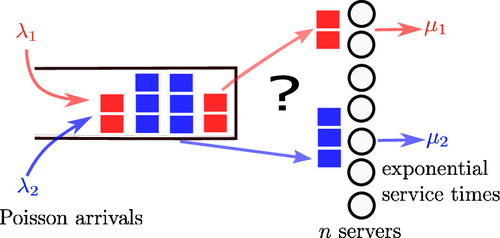
Notes. Type 1 jobs have arrival rate λ1, service rate μ1, and server need . Type 2 jobs have arrival rate λ2, service rate μ2, and server need .
The dynamics of the system are as follows. For each , type i jobs arrive to the system following a Poisson process with arrival rate λi. Upon arrival, a job either starts service immediately or waits in a centralized queue. When a type i job starts service, it leaves the queue and makes exclusive use of servers. The job leaves the system after receiving enough service. The service time of a type i job follows an exponential distribution with service rate μi. The service times and arrival events are independent. During the operation of the system, a scheduling policy is used to determine which set of jobs to serve at any time. The scheduling policy is allowed to be preemptive (i.e., we can put a job in service back to the queue and resume its service later).
We measure the performance of our scheduling policy based on mean waiting time as defined below. Let denote the waiting time of type i jobs in the steady state; then, the mean waiting time is defined as the steady-state expected waiting time averaged over all job types: that is,
1.2. Scaling Regimes
We study job delay in scaling regimes where the number of servers, n, goes to infinity. Specifically, we consider a sequence of systems with parameters scaling up jointly with n, and we analyze the growth/decrease rate of the mean waiting time. In the considered scaling regimes, the arrival rates λi and server needs are allowed to scale with n, whereas the service rate μi and the number of job types I stay constant. One key parameter for specifying a scaling regime is the slack capacity δ, defined as , which is the expected number of idle servers in the steady state. Slack capacity is used to specify the heaviness of traffic, which is alternatively specified by load ρ given by in the literature.
For expositional purposes, we now parameterize the scaling regimes in a specific way below to demonstrate our results. Our general model is presented in Section 3. Suppose for some exponents , and the total arrival rate . We refer to such scaling regimes as polynomial scaling regimes. To classify and visualize different polynomial scaling regimes, we aggregate all scaling regimes with the same pair into one point and plot all such points, as shown in Figure 2. We partition the set of exponent pairs into three triangles using the lines and . The corresponding scaling regimes in the upper left in Figure 2 are in general “heavier” than the scaling regimes in the lower right because the former regimes have larger work variability and smaller slack capacity. We comment that the point is analogous to the celebrated Halfin–Whitt regime introduced in Halfin and Whitt (1981) and that is analogous to the nondegenerate slowdown regime in Atar (2012) in traditional multiclass M/M/n models.
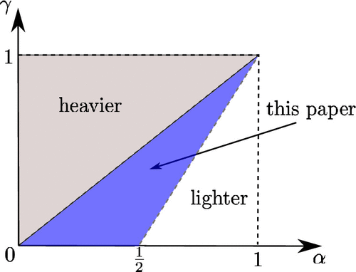
Notes. The traffic is heavier as we move to the upper left. The three triangles are partitioned by lines and .
In the polynomial scaling regimes where (indicated in white in Figure 2), Wang et al. (2021) proved that the queueing probability diminishes under FCFS when n gets large. In this paper, we further show that in these regimes, both the queueing probability and the mean waiting time diminish at a fast rate as n gets large under a large class of policies.
Although all reasonable policies perform well when , as we move on to polynomial scaling regimes with (marked in blue in Figure 2), different policies begin to show separations in their mean waiting times, as presented in our main results below.
1.3. Results
Here, we present our main results specialized to the polynomial scaling regimes. These results hold under several assumptions: , and .1 In Section 4, we will present the general results and comment on how they imply the results here.
Mean waiting time under FCFS. The exact order of the mean waiting time under FCFS is given by
(1)Mean waiting time lower bound. Under any policy, the mean waiting time satisfies
(2)Order-wise optimal policy. Consider a static priority policy that we call the smallest-need-first (SNF) policy, which preemptively prioritizes the jobs with smaller server needs. Then, the mean waiting time under SNF achieves the lower bound in (2): that is,
(3)Therefore, the SNF policy is order-wise optimal in the mean waiting time.
Comparing the mean waiting times under FCFS and under SNF, we can see that FCFS is strictly suboptimal when , and SNF improves upon FCFS by a factor of .
A key to proving the mean waiting time results above is the order-wise tight bounds on the expected workload we establish (Lemmas 1 and 2). In addition, although we consider the system under the traffic regime where , we still need to analyze “subsystems” that are in the lighter traffic regime. In this lighter regime, we show that the total server need decays faster than any polynomial (Lemma 8). All these lemmas hold under a very general class of policies, so they could be potentially relevant when we study policies other than FCFS and SNF.
1.3.1. Results on Queueing Probability.
As a by-product to our analysis, we further derive an upper bound on the queueing probability under any work-conserving policy, presented in Corollary 1, which significantly improves upon the queueing probability upper bound in Wang et al. (2021) in a slightly more constrained traffic regime.
1.3.2. Simulation Experiments.
The SNF policy we consider in our analysis is a preemptive priority policy. Preemption is sometimes undesirable in practice. Therefore, we use simulation experiments to also explore a nonpreemptive version of the priority policy, which we call the nonpreemptive smallest-need-first (SNF-NP) policy. SNF-NP serves a job with the smallest server need in the queue when enough numbers of servers free up. Our simulation experiments compare the mean waiting times under FCFS, SNF, and SNF-NP, along with a few other policies. The simulation results, presented in Section 10, show that SNF-NP has comparable performance with SNF, and both of them perform well relative to FCFS and other policies. We also investigate the weighted mean waiting times where jobs with larger server needs have larger weights. We find that SNF and SNF-NP remain competitive when the weights moderately depend on the server needs.
1.4. Technical Challenges
The main technical challenges in analyzing the considered multiserver-job system are rooted in the heterogeneity among job types in both their service rates and their server needs. Such heterogeneity makes the system dynamics multidimensional; neither the total number of jobs in service nor the total number of busy servers determine the current job departure rate. We comment that even for a classical multiclass M/M/n system, where there are multiple job types with different service rates but all job types have a server need of one, finding an optimal scheduling policy is known to be a hard problem, and solutions are available mostly in the so-called Halfin–Whitt heavy traffic regime through the diffusion control problem (Atar et al. 2004, Harrison and Zeevi 2004, Ata and Gurvich 2012). Compared with the classical multiclass M/M/n system, our multiserver-job system has an additional layer of intricacy because of the heterogeneous server needs, which makes it possible for the system to have servers idling while there are jobs waiting in the queue.
To address the challenges because of heterogeneity, our analysis relies on various state-space concentration results. State-space concentration is a phenomenon where the state concentrates around a subset of the state space in steady state, observed in queueing systems in heavy traffic or large-system regimes (Wang et al. 2018; Liu 2019; Liu and Ying 2020, 2022; Weng et al. 2020; Liu et al. 2022). In the multiserver-job system we consider, state-space concentration results are crucial for analyzing the system dynamics when the queue is nonempty. The scenario when the queue is nonempty is especially important to our scaling regimes because the queueing probability may not be diminishing even when the mean waiting time is diminishing. This contrasts with the analysis in the prior work of Wang et al. (2021), which focuses on diminishing queueing probability. Furthermore, our performance goal is to achieve the optimal order of the mean waiting time in large systems, deviating from the traditional performance goal of minimizing delay or certain long-run cost.
1.5. Organization of the Paper and the Relationship with the Conference Version
This paper is organized as follows. In Section 2, we review some additional related work that has not been discussed in Section 1. We present our model and assumptions in Section 3 and then formally state our three main theorems in Section 4. In Section 5, we give an overview of the proof structure and preliminaries of our main proof technique, the drift method. In Section 6, we state and prove Lemmas 1 and 2, which will be used to prove the three theorems in Sections 7, 8, and 9. In Section 10, we present the simulation results. Finally, we conclude the paper in Section 11.
This paper has the following differences from our previous conference version (Hong and Wang 2022). First, we have included a more comprehensive related work section (Section 2). Second, we have included proofs of some important lemmas and a theorem that were omitted because of the space limit in the conference paper. These are the proofs of Lemma 1, Lemma 2, and Theorem 1, which can be found in Section 6 and Section 7. Third, we have changed the name of the order-wise optimal policy that we propose from “P-priority” to “smallest need first” to better reflect the feature of the policy. Fourth, we have included more simulation results.
2. Related Work
In this section, we give a more detailed review of the prior work on multiserver-job models as well as some related models that are not covered in Section 1.
2.1. Multiserver-Job Model
As mentioned in Section 1, the majority of prior work on the multiserver-job model has either focused on characterizing stability conditions (Morozov and Rumyantsev 2016, Rumyantsev and Morozov 2017, Afanaseva et al. 2019, Grosof et al. 2020, Olliaro et al. 2023) or has been restricted to the highly specialized settings with two servers (Brill and Green 1984, Filippopoulos and Karatza 2008). There are relatively fewer papers that study the delay of the multiserver-job model, with different performance metrics. Wang et al. (2021) characterizes the queueing probability in a large multiserver-job model. Zychlinski et al. (2023) studies the optimal cumulative holding cost in a finite-horizon setting. The papers whose performance metrics are closest to our paper are Grosof et al. (2022a, b). Grosof et al. (2022a) characterizes the mean response time in a multiserver-job model under a policy called ServerFilling. Grosof et al. (2022b) proposes a variant of ServerFilling called ServerFilling shortest remaining service time (SRPT), which optimizes the mean response time in the traditional heavy traffic regime. The biggest distinction between their work and our work lies in the scaling regimes. In their work, the analysis of mean response time is asymptotically tight when the load of the system goes to one and the number of servers remains fixed; in contrast, we consider the scaling regimes where the load, number of servers, and server needs scale jointly. Another distinction is the assumptions on the server needs; their work assumes that the server needs can divide the total number of servers, whereas our work assumes that the maximal server need is small compared with the slack capacity.
2.2. Virtual Machine Scheduling
A problem related to the multiserver-job scheduling problem studied in this paper is the VM scheduling problem (see, e.g., Maguluri et al. 2012, 2014; Maguluri and Srikant 2014; Xie et al. 2015; Psychas and Ghaderi 2018, 2019; Stolyar and Zhong 2021). For the VM scheduling problem, typically the system consists of multiple servers, where each server has certain units of each type of resource (e.g., CPU, memory, storage). A VM job demands to occupy multiple units of each type of resource. Each VM job will be served on a single server. Some results for the VM scheduling problem in the traditional heavy traffic regime can be specialized to the multiserver job scheduling problem. To see this, consider a VM scheduling problem where the system consists of a single server and where there is a single resource type. Then, each unit of resource can be viewed as a server in the multiserver-job scheduling problem. With this specialization, the results in Maguluri et al. (2014) provide bounds on a linear combination of the queue lengths of different types of jobs. However, these bounds do not directly translate into bounds on mean job response time.
2.3. Multitask-Job Model
A multitask job is a job that consists of a batch of tasks that can run on servers in parallel, which is similar to a multiserver job in that both can occupy multiple servers at the same time. However, unlike a multiserver job, the tasks of a multitask job can have different run times and do not need to be executed simultaneously. The multitask job model has been considered under a wide variety of settings, and it is sometimes referred to as the batch arrival model (see, e.g., Miller 1959; Daw and Pender 2019; Daw et al. 2019, 2020). Recently, the multitask job model has also been extensively studied under the setting of parallel computing because of the popularity of large-scale data processing systems, such as MapReduce, Apache Hadoop, and Apache Spark (see, e.g., Weng and Wang 2020, Zubeldia 2020). The work closest to our work is Weng and Wang (2020), which shows diminishing queueing time for multiserver jobs in a load-balancing system where tasks of a job need to be dispatched to the queues at the servers upon arrival.
2.4. Dropping Model
When the multiserver-job system does not have any queueing space and allows incoming jobs to be dropped, it becomes a model that has been extensively studied in the literature, and we refer to it as the dropping model. In this model, one can design a dropping policy that decides whether to drop an incoming job or not based on the types of the incoming job and of the jobs currently in service. Under the policy that drops an incoming job only when it cannot fit into the servers (i.e., when its server need is larger than the number of available servers), the stationary distribution has a product form under exponentially distributed service times, as observed by Arthurs and Kaufman (1979). The results have been generalized by Whitt (1985) to allow jobs to demand multiple resource types (e.g., both CPU and input/output) and by van Dijk (1989) to allow general service time distributions. Tikhonenko (2005) further combined aspects of Whitt (1985) and van Dijk (1989). Different dropping policies, which mostly fall within the class of trunk reservation policies, have been designed to minimize the cost associated with dropping (Hunt and Kurtz 1994, Bean et al. 1995, Hunt and Laws 1997).
2.5. Streaming Model
The streaming model for a communication network resembles the multiserver-job model in many aspects. In a streaming model, the “servers” correspond to the bandwidth in the network, and the “jobs” are data flows, such as audio or video flows. Then, flows that require a fixed amount of bandwidth (Melikov 1996, Dasylva and Srikant 1999, Benameur et al. 2001, Ponomarenko et al. 2010), sometimes referred to as streaming flows, can be viewed as multiserver jobs. However, a communication network also features a network structure that the multiserver-job model does not have. A communication network usually has both streaming flows and flows that are flexible in their bandwidth needs, and streaming flows again operate in the dropping model. The performance metric in such a system typically combines the cost associated with dropping for streaming flows and the cost associated with delay for other flows.
3. Model
A basic description of the system parameters and dynamics has been given in Section 1. In this section, we provide formal descriptions of the scheduling policies, the system states, the scaling regime, and the concept of subsystems used in our analysis.
3.1. Scheduling Policies
A scheduling policy decides which jobs to put into service at any moment of time. We are interested in the following two policies.
FCFS. Jobs are placed onto servers in a first come, first serve fashion until either the next job in queue does not fit or all the jobs are in service.
SNF. Recall that the job types are indexed in a way such that . We assign priorities to job types such that a smaller index has a higher priority. Whenever there is a job arrival or departure, SNF preempts all the jobs in service and determines a new schedule from scratch. SNF starts from job type 1 and places as many type 1 jobs as possible onto servers. After this, if there are still servers available, SNF goes to the next priority level, type 2, and places as many type 2 jobs as possible onto servers. This procedure continues until no more jobs in the queue can fit into the servers.
3.2. System State
Under FCFS or SNF, a Markovian representation of the system state can be described as follows. The state u of the Markov chain is an ordered list of the jobs in the system, sorted in their order of arrival, and each entry of u describes the type of the corresponding job and whether the job is in service or not. Let the state space be denoted as . Although the state space is infinite dimensional, in our analysis, we typically only need to focus on three I-dimensional vectors defined below.
For any time t and each job type i, let denote the number of type i jobs in the system, denote the number of type i jobs in service, and denote the number of type i jobs waiting in the queue. Note that because the total number of servers in use cannot exceed n and we cannot serve more jobs than there are in the system, we have the following constraints:
Let , and be random variables that follow the corresponding steady-state distributions when they exist. We sometimes use vector representations of these quantities for convenience. For example, we write . We define the vectors , and in a similar way. Note that these random elements correspond to the n server system, and thus, their distributions depend on n. Throughout this paper, for conciseness, we often omit the in the steady-state random elements except in theorem or lemma statements.
Recall that the waiting time for a job is the total time that the job spends in the queue. Our performance metric is the mean waiting time , given by
Bounding the mean waiting time is thus equivalent to bounding the expected total queue length.
3.3. Scaling Regimes
Recall that we consider scaling regimes where the number of servers, n, goes to infinity and the arrival rates λi and server needs are allowed to scale with n, whereas the service rate μi and the number of job types I stay constant. The scaling regimes are specified by the slack capacity , the maximal server need , and another parameter called the work variability: . Work variability reflects the variability of the “work” caused by job arrivals in terms of server-time product, which is in expectation for each type i job. To help later presentation, we also define the load brought by type i jobs ρi as .
We state our assumptions below. Throughout the paper, denotes natural logarithm.
(
(
(
Assumption 1 guarantees that the traffic is not too light, whereas Assumption 2 guarantees that the system is stable under FCFS and SNF. In the simplified setting of Section 1 where and , the first two assumptions correspond to and , which exclude the white and gray parts in Figure 2, respectively. Assumption 3 states that the load brought by the maximal-need jobs is not too small. To understand the right-hand side expression in Assumption 3, note that it is automatically satisfied when . For example, when , then it suffices to have . However, when the traffic becomes heavier (i.e., when becomes smaller), Assumption 3 in (7) can be much weaker than .
To have an intuitive view of the magnitudes of the parameters, we give the following asymptotics: , and ; they can be verified from the assumptions.
3.4. Subsystems
When we analyze SNF and prove the lower bound for all policies, we frequently use the concept of the ith subsystem, which is the system that has all type j jobs in the original system with and removes all type k jobs with . In the ith subsystem, the slack capacity becomes , and the work variability becomes . Note that and . The maximal server need in the ith system is because .
As i increases, the load of the ith subsystem gets heavier because δi becomes smaller. There is a critical index such that
4. Main Results
In this section, we first present our main results under the scaling regimes we specify in Section 3 as Theorems 1, 2, and 3. Then, we comment on how the theorems subsume the results in Section 1.3.
(
Consequently,
(
(
We have a more general bound for the SNF policy that holds without Assumption 3. Interested readers can refer to Online Appendix A.
The results appearing in Section 1.3 are direct consequences of the above theorems. Recall that in the polynomial scaling regimes, we have , , and . The requirement implies Assumptions 1 and 2; the requirement implies Assumption 3. Under these assumptions, the bounds in Theorems 1, 2, and 3 hold. It can be verified that , so the expression in (11) has the order ; the critical index , so the expression in (12) and (13) equals .
5. Proof Road Map and Drift Method Preliminaries
We organize our proofs of the main results as follows; we first prove two important bounds for a quantity called workload given by in Lemmas 1 and 2, respectively. Then, we convert the workload bounds to the waiting time bounds in Theorems 1 and 2 using properties of FCFS and a linear programming relaxation. For Theorem 3, we analyze SNF by considering each ith subsystems for . Some subsystems only need Lemma 1 and Lemma 2, whereas others require the addition of Lemma 8.
Our proof approach is closely related to the recently developed drift method (Eryilmaz and Srikant 2012, Maguluri and Srikant 2016). The drift method allows us to extract information from a continuous-time Markov chain on state-space by computing the drift of different test functions. Because S(t) is a Markov chain with countable state space and bounded transition rates, we can define the drift of any function f as
We call the operator G the generator of the Markov chain.
For a multiserver-job system, let I-dimensional real vectors be possible realizations of state descriptors and , where recall that is the vector of the number of jobs in the system at time t and is the vector of the number of jobs in service at time t. We focus on f that only depends on x (i.e., ). The drift of f is of the form
We frequently use the following relation regarding the drift
Heuristically, this is because when and follow the stationary distribution, and also follow the stationary distribution; so, and have the same expectation. Rigorously speaking, this relation only holds for well-behaved functions and Markov processes. The conditions under which the relation holds are discussed in detail in Online Appendix B. Throughout the paper, we assume (16) holds for all f that we consider.
6. Workload Bounds
In this section, we prove two bounds for a quantity called workload given by . These bounds are fundamental to the proofs of the main theorems. In Lemma 1, we give a lower bound on the expected workload applicable to any policy. In Lemma 2, we give upper bounds on the expected workload under any -work-conserving policy, a class of policies defined in Definition 1. After stating these two lemmas, we go through preliminaries for the proofs. Finally, we show the full proof of the two lemmas at the end of the section.
(
We call a policy -work conserving if the following equation holds
Here, is equal to the number of busy servers at time t, whereas , which we call the total server need, is the potential number of busy servers if we can put all jobs at time t into service. Therefore, under a -work-conserving policy, either all jobs are in service, or there are at most idling servers. Under any -work-conserving policy, one can show that the system is stable when (Assumption 2) holds. In particular, the system is stable under both FCFS and SNF.
(
When Assumption 1 is satisfied (i.e., when ), the workload upper bound in Lemma 2 coincides with the workload lower bound in Lemma 1 order wise, which implies that the expected workload . Note that in this case, although the expected workload under all -work-conserving policies has the same order, the mean waiting time can vary among policies, as shown for FCFS and SNF in Theorems 1 and 3.
6.1. Preliminaries for Lemma 1 and Lemma 2
Our proofs focus on bounding the normalized work, defined as
Therefore, bounding the expected workload is equivalent to bounding the steady-state expectation of the normalized work .
We break into three terms:
The major difficulty during the proofs is bounding the expectation of the positive part . This relies on the relation that as introduced in Section 5. In our proofs, we choose f to be piecewise quadratic functions to bound on the term
Because , we will be able to bound if we are able to give an accurate estimate of the number of busy servers when the normalized work . To get a precise estimate, we exploit the state-space concentration result that says for each , Xi cannot be much smaller than (i.e., is small with high probability). Formally, this state-space concentration is established by Lemma 3, whose proof uses a sample-path coupling argument and is given in Online Appendix C.
Consider the multiserver-job system with n servers. For any nonnegative vector independent of n, let , and
For any ,
(23)For any and such that and any ,
(24)Let to be the negative part of . Then,
(25)
6.2. Proofs of Lemma 1 and Lemma 2
In this section, we show the full proofs of Lemma 1 and Lemma 2.
Recall that in Section 6.1, we have shown that , where is the normalized work given by and . Therefore, our goal is equivalent to lower bounding . To do this, we first perform the following decomposition:
Here, is a properly chosen small number to be specified later. We bound the positive part and the negative part separately using different techniques.
We bound by analyzing the Lyapunov drift of a function defined below. Let denote possible realizations of the state descriptors . Then, f is defined as
We will utilize the relation , which is implied by Lemma 9 in Online Appendix B if we have . Because grows linearly fast as x gets large, follows if we have for all . On the other hand, the lemma statement holds trivially if for some i.
To calculate , we first decompose the drift Equation (15) in the following way:
It is easy to see that the partial derivatives of f appearing in the first term are given by
To bound the remaining two terms, observe that
Plugging the above inequalities into the decomposition of the drift (26) and taking expectation on both sides because , we have
The inequality still holds when we let inside the expectation:
Here, we are implicitly exchanging and , which is legal by the dominated convergence theorem given that the random variable inside the expectation is dominated by another random variable with a finite expectation, . Using the facts that and , we get
By Lemma 3 with , we have Note that this K satisfies . We take ; then, . Moreover, observe that , so
The lower bound for negative part follows from Lemma 3(c), which shows that . Because is a monotonically decreasing function and ,
Therefore, combining (31), (32), and the fact that , we have
Recall that in Section 6.1, we have shown that , where is the normalized work given by and . Moreover, we have
We bound by analyzing the Lyapunov drift of a function defined below. Let denote possible realizations of the state descriptors . We define f as
This proof relies on the relation that , which is justified by Lemma 11 in Online Appendix B. To calculate , we decompose the drift Equation (15) in the following way:
It is easy to see that in the first term of (34) is given by
The other two terms in (34) can be bounded by constants independent of x and z as below:
Because , plugging the last inequality into the decomposition of the drift, (34), and taking expectation on both sides of (34), we get
Observe that because , the second term in (35) can be straightforwardly computed as
Rearranging the terms, we get the following key equation; for any real number ,
Now, suppose we are able to show that
We devote the remainder of this proof to proving (38). The idea here is to use the following two events to further partition the probability space:
Case 1. Event happens. Observe that the term in (39) is nonzero only when and event happens, which implies that
Adding up the above two inequalities and rearranging the terms yield
(42)When the above inequality holds, we can invoke the definition of the -work-conserving policy and the fact that to get
(43)(44)Case 2. Event happens. To bound the term in (40), we need to analyze the probability of event . Consider Lemma 3 with . It can be verified that . Let . Then, we have
Note that this choice of K2 satisfies .
With the upper bound , we bound the term in (40) in the following way. Observe that . Furthermore, when the event occurs, and . Consequently, we have the following two inequalities:
We can rearrange the above inequalities into a similar form as (44):
(45)where we have used the fact that .Case 3. Event happens. Lastly, we bound the term in (41). Observe that implies that , so a -work-conserving policy will make sure that . Therefore,
(46)
Combining the results in three cases (44), (45), and (46), we have
Therefore, we have shown (38) with . By (37), we conclude that
Next, we simplify (48) based on the order of δ. When , we take and get
When , we have for some C > 0 and n large enough. Because , we get for n large enough. Taking yields , so
This finishes the proof. □
7. Proof of Theorem 1 (Waiting Times Under FCFS)
7.1. Proof Overview and Lemmas
We prove Theorem 1 in this section. We first present some intuition and state two lemmas. Then, we give a proof of the theorem using the lemmas. We leave the proofs of the lemmas to Online Appendix D.
The analysis of FCFS is based on the intuition that, under FCFS, the number of type i jobs in the queue is approximately proportional to its arrival rate λi: that is,
This intuition is formalized by considering a modified-FCFS policy, which serves the jobs in an FCFS order but will not serve the next job until there are at least idle servers. In Lemma 4, we prove that under modified FCFS, (49) holds exactly, so the expected queue length of each type of jobs can be computed using the above argument. Moreover, when n is large, we expect modified FCFS to be a good approximation of FCFS. In fact, we can define an upper-bounding system as the multiserver-job system with n servers under modified FCFS and define a lower-bounding system as the multiserver-job system with servers under modified FCFS. In Lemma 5, we prove that the queue length of each type of jobs in the original system is sandwiched between those in the two modified systems. Because the two modified systems themselves are very close to each other, we get a tight characterization of FCFS.
For both the upper-bounding system and the lower-bounding system, we have
7.2. Proof of Theorem 1
Recall that by Little’s law, and . To characterize , Lemma 5 suggests that we only need to characterize and , the queue lengths in the lower-bounding system and the upper-bounding system, for each .
Observe that the lower-bounding system has servers, with slack capacity . Because , we can apply Lemmas 1 and 4 to get
Recall the facts introduced in Section 3 that and , so we have . Therefore, the above equation implies that . By Lemma 4,
For the upper-bounding system, observe that it has n server and slack capacity δ and that it operates under an -work-conserving policy. Applying the workload upper bound in Lemma 2 yields
Following a similar argument as in the lower-bounding system, we have
Therefore, by Lemma 5, we have
8. Proof of Theorem 2 (Mean Waiting Time Lower Bound)
Recall that by Little’s law, . Therefore, it suffices to show a lower bound on the total queue length. We fix a policy in the original system. For any i with , we consider the ith subsystem by ignoring all job types with index greater than i. In the ith subsystem, it is always possible to achieve the same ’s for by imitating the service decisions taken by the original system. Therefore, we have , where the right-hand side expression is the workload lower bound of the ith subsystem according to Lemma 1. Then, the expected waiting time is lower bounded by the optimal value of the following linear programming problem:
Therefore,
The proof of the lower bound provides some intuitions for choosing the SNF policy. We consider the simple case where . By (57), the total queue length order wise achieves the lower bound when the queue consists of jobs with the largest server needs, suggesting that we should give low priorities to those jobs. This is in a similar spirit to the famous SRPT policy for single-server jobs, which leaves the jobs with large remaining service times in the queue (see, e.g., Harchol-Balter 2013).
9. Proof of Theorem 3 (Mean Waiting Time Under SNF)
To understand the behavior under the SNF policy, one key observation is that for each , the type i jobs are unaffected by type j jobs with j > i. As a result, we can learn about the original system by analyzing each ith subsystem, which is obtained by removing all jobs of type j with j > i. Some subsystems are under relatively heavier traffic or more precisely, subject to , whereas some subsystems are under lighter traffic. For those subsystems under relatively heavier traffic, Lemmas 1 and 2 are enough for use; for those subsystems under lighter traffic, we sometimes use Lemma 8 below, which is a more refined bound on the expected total server need , proven based on the two tail bounds in Lemmas 6 and 7. The proofs of Lemma 6, Lemma 7, and Lemma 8 are in Online Appendix E.
Consider the multiserver-job system with n servers satisfying (Assumption 2). Letting , under any -work-conserving policy, the normalized work has the following tail bound; for any ϵ such that , there exists and such that for any ,
Consider the multiserver-job system with n servers satisfying (Assumption 2). Letting , under any -work-conserving policy, the total server need has the following tail bound; there exists α2 and β2 with and such that for any ,
The proof technique of the two lemmas is using state-space concentration successively. Lemma 6 relies on the state-space concentration implied by Lemma 3, whereas Lemma 7 relies on the state-space concentration implied by Lemma 3 and Lemma 6.
As a consequence of the first two lemmas, we can give a bound on the expectation of the total server need in a different traffic regime than what is assumed in Assumption 1. This is useful for analyzing the dynamics of subsystems under SNF.
(
As a quick digression, with Lemma 7, we can prove an upper bound on the queueing probability in Corollary 1. We comment that this queueing probability bound significantly improves on the bound in Wang et al. (2021) in a slightly more constrained traffic regime.
(
Now, we are ready to prove Theorem 3.
Recall that by Little’s law, we have that , and thus, it suffices to bound ’s. We bound separately for each as follows:
Case 1. . Applying Lemma 2 to the ith subsystem, we have
Therefore,
Case 2. and . Applying Lemma 2 to the ith subsystem, we have
Combining the above equation with (63) and the facts that and , we have
Case 3. and . We first show that . To see this, observe that implies i < I, so . By Assumption 3, we have
(64)
Therefore, we can apply Lemma 8 to the ith subsystem to get
Combining the three cases, we get
Finally, note that I and are independent of n during scaling, and for some . Therefore,
10. Simulation Results
10.1. Experiment 1: Comparing SNF and SNF-NP with FCFS
Our theoretical analysis shows that there is an order gap in mean waiting times under FCFS and SNF for the scaling regimes satisfying Assumptions 1, 2, and 3. Here, we complement our asymptotic results by comparing the simulated performances of SNF and FCFS in finite systems. We also simulate the nonpreemptive variant of SNF, which we call SNF-NP. SNF-NP identifies jobs in the queue that can fit into the idle servers and prioritizes those with the smallest server needs for service.
We run the simulation experiments under two sets of parameters.2 Parameter Set One satisfies all three assumptions, whereas Parameter Set Two does not satisfy Assumption 3. The parameters are specified in Figure 3. We can see that both SNF and SNF-NP outperform FCFS by a large margin. In particular, the ratio between the mean waiting times of FCFS and SNF is always greater than 3 when , and it gets to as large as 40.0 under Parameter Set One and 54.4 under Parameter Set Two.
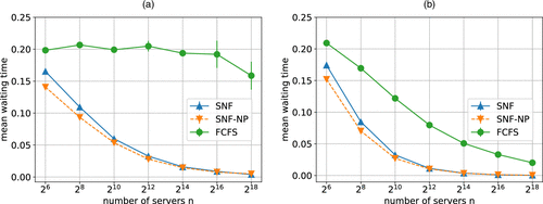
Notes. (a) The mean waiting times under Parameter Set One. There are three job types, with service rates and server needs given by ; ; and . Slack capacity . The arrival rates are chosen so that the loads satisfy . (b) The mean waiting times under Parameter Set Two. There are three job types with the same service rates, server needs, and slack capacity as Parameter Set One. The arrival rates are chosen so that the loads satisfy .
A secondary finding is that SNF-NP performs slightly better than SNF. This phenomenon is also observed in the next few experiments, the reason for which is unclear from our current theory. We hypothesize that under SNF, the jobs with large server needs sometimes do not fit into the remaining servers after they are preempted, leading to more idle servers. SNF-NP alleviates this issue by prohibiting preemption. However, this advantage of SNF-NP is moderate because the maximal server need is smaller than the slack capacity in our scaling regimes.
10.2. Experiment 2: Comparing with More Policies
One limitation of our policies, SNF and SNF-NP, is that they do not utilize the service rate information. Although we can show the order-wise optimality of SNF, our analysis is restricted to the scaling regimes where the service rates μi’s do not scale with n (i.e., the values of μi’s cannot be too large or small). When the values of μi’s vary significantly across different job types, it becomes questionable whether scheduling jobs solely based on server needs is the most effective way. For example, it could be more natural to prioritize jobs with smaller expected sizes, defined as for jobs of type i.
Another aspect not considered in SNF and SNF-NP is the packing effect; SNF and SNF-NP do not aim to minimize the number of idle servers, , when choosing the subset of jobs to serve, which might harm the mean waiting times. Furthermore, the approach of SNF and SNF-NP is somewhat contrary to common bin-packing algorithms. For instance, the best-fit algorithm prioritizes packing jobs with larger server needs rather than those with smaller server needs.
Given the motivation discussed, we compare the mean waiting times of SNF and SNF-NP with the following policies that utilize the expected sizes or consider the packing effect.
Smallest size first (SSF). SSF prioritizes jobs with smaller values of preemptively; it is the special case of the rule in Zychlinski et al. (2023), with c being the all-one vector.
Largest need first (LNF). LNF prioritizes jobs with larger server needs preemptively; it can be seen as following the best-fit algorithm to improve the packing.
ServerFilling Gittins (SFG). SFG is a policy designed for multiserver job models with general service time distributions under the assumption that the number of servers n and the server needs are powers of two (Grosof et al. 2022b). Adapted to our setting, SFG schedules jobs based on both the expected sizes and the server needs, aiming to prioritize jobs with smaller expected sizes while optimizing packing.
We simulate the three policies described above along with SNF, SNF-NP, and FCFS. The parameters are similar to those used in Figure 3(a), with two modifications; we set to be a power of two and increase the service rates for job types 2 and 3. The simulations are conducted under two sets of parameters with different service rates, namely Parameter Set Three and Parameter Set Four, as illustrated in Figure 4, (a) and (b), respectively.
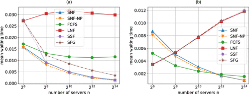
Notes. (a) The mean waiting times under Parameter Set Three. There are three job types with service rates and server needs ; ; and . Slack capacity . The arrival rates are chosen according to loads . (b) The mean waiting times under Parameter Set Four. There are three job types with service rates and server needs ; ; and . Slack capacity . The arrival rates are chosen according to loads .
From Figure 4, we can see that LNF is always worse than SNF and SNF-NP for . The performance of SSF depends on its priority order. When it gives type 3 jobs the lowest priority (e.g., when in Figure 4(a)), it performs similarly to SNF and SNF-NP; otherwise, it performs similarly to LNF (for all n in Figure 4(b)). The performance of SFG lies between LNF and SSF. None of the three policies outperform SNF and SNF-NP for .
The comparison between LNF and SFG with SNF and SNF-NP indicates that considering the packing effect does not bring much benefit to the mean waiting time in the scaling regimes of the two examples in Figure 4. This outcome aligns with our expectations because the slack capacity here is larger than the maximal server needs, which ensures that any -work-conserving policy maintains enough busy servers to quickly reduce the workload even if the packing is not optimal.
On the other hand, the relationships between SSF, LNF, and SNF are more interesting; they suggest that in these examples, a policy is likely to have small mean waiting times when the maximal-need jobs (i.e., type 3 jobs) are served with the lowest priority, even if those jobs may have large service rates and the smallest expected sizes, as we can see from the data points in Figure 4(b) with . Fully understanding this phenomenon is outside the scope of our theory because we assume that the service rates do not scale with n, whereas in Figure 4(b), the service rates can be even larger than the server needs. In Online Appendix F, we give further details of Experiment 2 and provide some preliminary hypotheses about this phenomenon. There we make an interesting observation that in the setting of Experiment 2, the workload is considerably smaller under SNF than under LNF. Intuitively, SNF make the jobs with large service rates and large server needs stay longer in the system by giving them low priorities; those jobs will help keep more servers busy during periods when there are fewer jobs in the system.
10.3. Experiment 3: Mean Waiting Times Weighted by Server Needs
We have been focusing on the unweighted mean waiting time. However, sometimes we may want to give the jobs with larger server needs larger weights—for example, when each multiserver job consists of many unit-server-need components and one cares about the mean waiting time averaged over the components.
In Figure 5, we consider mean waiting times weighted by (Figure 5(a)) and weighted by (Figure 5(b)) under Parameter Set Three (the same model parameters as Figure 4(a)). We can see that when the mean waiting times are weighted by , for , SFG outperforms other policies followed by SNF-NP, SNF, SSF, and lastly, LNF and FCFS. When the mean waiting times are weighted by , LNF shows the best performance for all n followed by SFG and other policies.
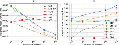
Notes. (a) The weight is for each type i. (b) The weight is for each type i.
These two simulations indicate that generally, when the weights of the mean waiting times depend on the server needs, other policies could outperform SNF and SNF-NP. Nevertheless, as shown in Figure 5(a), SNF and SNF-NP still perform reasonably well when the weights moderately depend on the server needs.
11. Conclusion and Future Work
In this paper, we establish order-wise sharp bounds on the mean waiting times of multiserver jobs under the FCFS policy and the SNF policy. We also prove a lower bound for the mean waiting times under all policies. These bounds imply the order-wise optimality of SNF and the strict suboptimality of FCFS.
Our analysis has two steps; we first prove the workload bounds stated in Lemmas 1 and 2 for a general class of policies using the drift method, along with some novel state-space concentration arguments. Then, we use the workload bounds to analyze the mean waiting times under FCFS and SNF, and we prove a lower bound for the mean waiting times under all policies.
Apart from the theoretical analysis, we also perform simulation experiments. We first demonstrate through simulations the performance improvement of SNF compared with FCFS in finite systems and the fact that SNF-NP, the nonpreemptive variant of SNF, has comparable performance with SNF. We also compare SNF and SNF-NP with other policies that utilize the service rate information or consider packing effects. We find that in our examples, when the number of servers is large, SNF and SNF-NP outperform those policies. Finally, we investigate the weighted mean waiting times under these policies, where jobs with larger server needs have larger weights. We find that in this case, other policies could outperform SNF and SNF-NP, but SNF and SNF-NP still perform reasonably well when the weights moderately depend on the server needs.
There are several interesting directions for future work.
Derive a tighter bound on the mean waiting time under SNF when Assumption 3 is violated.
Design a policy that achieves order-wise optimality in the many-server scaling limit without the maximal server need (assumption Assumption 2).
Understand why the performance of SNF-NP appears to be slightly better than SNF.
Extend the analysis to the settings where the service rates scale with n; this could help us understand why SNF and SNF-NP outperform other policies in Experiment 2.
1 We use the standard Bachmann–Landau notation. Consider two sequences a(n) and b(n) (or simply a and b), where b(n) is positive for large-enough n. Then, if ; if ; if , which is equivalent to ; if , which is equivalent to ; and if a satisfies both and .
2 In all of our experiments, we run a long-enough trajectory to estimate the mean and the confidence interval for each data point. The confidence interval is estimated through batch means method (see Asmussen and Glynn 2007). We run a long trajectory, divide it into 20 batches, and calculate the standard deviation of the means across the batches; the radius of the confidence interval is 1.96 times the standard deviation estimated from the batch means.
References
- (2016) Tensorflow: A system for large-scale machine learning. Keeton K, Roscoe T, eds. Proc. USENIX Conf. Operating Systems Design Implementation (OSDI) (USENIX Association, Berkeley, CA), 265–283.Google Scholar
- (2019) Stability analysis of a multi-server model with simultaneous service and a regenerative input flow. Methodology Comput. Appl. Probab. 22(4):1–17.Google Scholar
- (1979) Sizing a message store subject to blocking criteria. Arató M, Butrimenko A, Gelenbe E, eds. Proc. Internat. Sympos. Computer Performance Model. Measurements Evaluation (IFIP Performance) (North-Holland, Amsterdam), 547–564.Google Scholar
- (2007) Steady-State Simulation (Springer, New York), 96–125.Google Scholar
- (2012) On optimality gaps in the Halfin–Whitt regime. Ann. Appl. Probab. 22(1):407–455.Google Scholar
- (2012) A diffusion regime with nondegenerate slowdown. Oper. Res. 60(2):490–500.Link, Google Scholar
- (2004) Scheduling a multi class queue with many exponential servers: Asymptotic optimality in heavy traffic. Ann. Appl. Probab. 14(3):1084–1134.Google Scholar
- (1995) Asymptotic analysis of single resource loss systems in heavy traffic, with applications to integrated networks. Adv. Appl. Probab. 27(1):273–292.Google Scholar
- (2001) Integrated admission control for streaming and elastic traffic. Smirnov MI, Crowcroft J, Roberts J, Boavida F, eds. Internat. Workshop Quality Future Internet Services (QofIS) (Springer, Berlin, Heidelberg), 69–81.Google Scholar
- (1984) Queues in which customers receive simultaneous service from a random number of servers: A system point approach. Management Sci. 30(1):51–68.Link, Google Scholar
- (1999) Bounds on the performance of admission control and routing policies for general topology networks with multiple call centers. Ephremides T, Tripathi SK, eds. Proc. IEEE Internat. Conf. Comput. Comm. (INFOCOM), vol. 2 (IEEE Computer Society, Alamitos, CA), 505–512.Google Scholar
- (2019) On the distributions of infinite server queues with batch arrivals. Queueing Systems 91(3–4):367–401.Google Scholar
- (2020) Non-stationary queues with batch arrivals. Preprint, submitted August 3, https://arxiv.org/abs/2008.00625.Google Scholar
- (2019) How to staff when customers arrive in batches. Preprint, submitted July 30, https://arxiv.org/abs/1907.12650.Google Scholar
- (2012) Asymptotically tight steady-state queue length bounds implied by drift conditions. Queueing Systems 72(3–4):311–359.Google Scholar
- (2008) A two-class parallel system with general service times of the parallel class. J. Comput. System Sci. 74(6):942–964.Google Scholar
Google (2022) Google Kubernetes engine. The most scalable and fully automated Kubernetes service. Accessed January 22, 2023, https://cloud.google.com/kubernetes-engine.Google Scholar- (2020) Stability for two-class multiserver-job systems. Preprint, submitted October 1, https://arxiv.org/abs/2010.00631.Google Scholar
- (2022a) WCFS: A new framework for analyzing multiserver systems. Queueing Systems 102(1):143–174.Google Scholar
- (2022b) Optimal scheduling in the multiserver-job model under heavy traffic. ACM SIGMETRICS Performance Evaluation Rev. 51(1):99–100.Google Scholar
- (1981) Heavy-traffic limits for queues with many exponential servers. Oper. Res. 29(3):567–588.Link, Google Scholar
- (2013) Performance Modeling and Design of Computer Systems: Queueing Theory in Action, 1st ed. (Cambridge University Press, New York).Google Scholar
- (2004) Dynamic scheduling of a multiclass queue in the Halfin–Whitt heavy traffic regime. Oper. Res. 52(2):1–31.Google Scholar
- (2022) Sharp waiting-time bounds for multiserver jobs. Naghizadeh P, Sun Y, eds. ACM Internat. Sympos. Mobile Ad Hoc Networking Comput. (MobiHoc) (ACM, New York), 161–170.Google Scholar
- (1994) Large loss networks. Stochastic Processes Their Appl. 53(2):363–378.Google Scholar
- (1997) Optimization via trunk reservation in single resource loss systems under heavy traffic. Ann. Appl. Probab. 7(4):1058–1079.Google Scholar
- (2018) A model-based approach to streamlining distributed training for asynchronous SGD. Wildani A, Wang M, eds. IEEE Internat. Sympos. Model. Anal. Simulation Comput. Telecomm. Systems (MASCOTS) (IEEE Computer Society, Los Alamitos, CA), 306–318.Google Scholar
- (2019) Steady state analysis of load balancing algorithms in the heavy traffic regime. PhD thesis, Arizona State University, Tempe.Google Scholar
- (2020) Steady-state analysis of load-balancing algorithms in the sub-Halfin–Whitt regime. J. Appl. Probab. 57(2):578–596.Google Scholar
- (2022) Universal scaling of distributed queues under load balancing in the super-Halfin–Whitt regime. IEEE/ACM Trans. Networking 30(1):190–201.Google Scholar
- (2022) Steady-state analysis of load balancing with Coxian-2 distributed service times. Naval Res. Logist. 69(1):57–75.Google Scholar
Maguluri ST, Srikant R (2014) Scheduling jobs with unknown duration in clouds. IEEE/ACM Trans. Netw. 22(6):1938–1951. Google Scholar- (2016) Heavy traffic queue length behavior in a switch under the maxweight algorithm. Stochastic Systems 6(1):211–250.Link, Google Scholar
- (2012) Stochastic models of load balancing and scheduling in cloud computing clusters. Greenberg AG, Sohraby K, eds. Proc. IEEE Internat. Conf. Comput. Comm. (INFOCOM) (IEEE Computer Society, Los Alamitos, CA), 702–710.Google Scholar
- (2014) Heavy traffic optimal resource allocation algorithms for cloud computing clusters. Performance Evaluation 81:20–39.Google Scholar
- (1996) Computation and optimization methods for multiresource queues. Cybernetics Systems Anal. 32(6):821–836.Google Scholar
- (1959) A contribution to the theory of bulk queues. J. Roy. Statist. Soc. Ser. B Methodological 21(2):320–337.Google Scholar
- (2016) Stability analysis of a MAP/M/s cluster model by matrix-analytic method. Fiems D, Paolieri M, Platis AN, eds. Eur. Workshop Comput. Performance Engrg. (EPEW), vol. 9951 (Springer, Cham, Switzerland), 63–76.Google Scholar
- (2023) The saturated multiserver job queuing model with two classes of jobs: Exact and approximate results. Performance Evaluation 162:102370.Google Scholar
- (2010) Performance Analysis and Optimization of Multi-Traffic on Communication Networks (Springer Science & Business Media, New York).Google Scholar
- (2018) On non-preemptive VM scheduling in the cloud. SIGMETRICS Perform. Eval. Rev. 46(1):67–69.Google Scholar
- (2019) Scheduling jobs with random resource requirements in computing clusters. Rawat D, Tang J, eds. Proc. IEEE Internat. Conf. Comput. Comm. (INFOCOM) (IEEE Computer Society, Los Alamitos, CA), 2269–2277.Google Scholar
- (2017) Stability criterion of a multiserver model with simultaneous service. Ann. Oper. Res. 252(1):29–39.Google Scholar
- (2021) A service system with packing constraints: Greedy randomized algorithm achieving sublinear in scale optimality gap. Stochastic Systems 11(2):83–111.Link, Google Scholar
- (2005) Generalized Erlang problem for service systems with finite total capacity. Problems Inform. Transmission 41(3):243–253.Google Scholar
- (2020) Borg: The next generation. Bilas A, Magoutis K, Markatos EP, Kostic D, Seltzer MI, eds. Proc. Eur. Conf. Comput. Systems (EuroSys) (ACM, New York), 30:1–30:14.Google Scholar
- (2020) Zero-wait load balancing with sparse messaging. Oper. Res. Lett. 48(3):368–375.Google Scholar
- (1989) Blocking of finite source inputs which require simultaneous servers with general think and holding times. Oper. Res. Lett. 8(1):45–52.Google Scholar
- (2015) Large-scale cluster management at Google with Borg. Réveillère L, Harris T, Herlihy M, eds. Proc. Eur. Conf. Comput. Systems (EuroSys) (ACM, New York), 18:1–18:17.Google Scholar
- (2021) Zero queueing for multi-server jobs. Proc. ACM Measurement Anal. Comput. Systems 5(1):7.Google Scholar
- (2018) Heavy-traffic delay insensitivity in connection-level models of data transfer with proportionally fair bandwidth sharing. ACM SIGMETRICS Perform. Eval. Rev. 45(3):232–245.Google Scholar
- (2020) Achieving zero asymptotic queueing delay for parallel jobs. Proc. ACM Measurement Anal. Comput. Systems 4(3):42.Google Scholar
- (2020) Optimal load balancing with locality constraints. Proc. ACM Measurement Anal. Comput. Systems 4(3):45.Google Scholar
- (1985) Blocking when service is required from several facilities simultaneously. ATT Tech. J. 64(8):1807–1856.Google Scholar
- (2015) Power of d choices for large-scale bin packing: A loss model. ACM SIGMETRICS Performance Evaluation Rev. 43(1):321–334.Google Scholar
- (2020) Delay-optimal policies in partial fork-join systems with redundancy and random slowdowns. Proc. ACM Measurement Anal. Comput. Systems 48(1):39–40.Google Scholar
- (2023) Managing queues with different resource requirements. Oper. Res. 71(4):1387–1413.Link, Google Scholar