


Can Customer Arrival Rates Be Modelled by Sine Waves?
Abstract
Customer arrival patterns observed in the real world typically exhibit strong seasonal effects. It is therefore natural to ask, can a nonhomogeneous Poisson process (NHPP) with a rate function that is the simple sum of sinusoids provide an adequate description of reality? If so, how can the sinusoidal NHPP be used to improve the performance of service systems? We empirically validate that the sinusoidal NHPP is consistent with arrival data from two settings of great interest in service operations: patient arrivals to an emergency department and customer calls to a bank call centre. This finding provides rigorous justification for the use of the sinusoidal NHPP assumption in many existing queuing models. We also clarify why a sinusoidal NHPP model is more suitable than the standard NHPP when the underlying arrival pattern is aperiodic (e.g., does not follow a weekly cycle). This is illustrated using data from a car dealership and also via a naturalistic staffing simulation based on the call centre. On the other hand, if the arrival pattern is periodic, we explain why both models should perform comparably. Even then, the sinusoidal NHPP is still necessary for managers to use to verify that the arrival pattern is indeed periodic, a step that is seldom performed in applications. Code for fitting the sinusoidal NHPP to data is provided on GitHub.
History: This paper has been accepted for the Service Science/Stochastic Systems Joint Special Issue.
Funding: N. Chen was supported by Natural Sciences and Engineering Research Council of Canada Discovery [Grant RGPIN-2020-04038]. H. Shen was supported by China Ministry and Science and Technology [Grant 2022SQGH10861], Hong Kong Special Administrative Region University Grants Council Collaborative Research Fund [Grant C7162-20G], University of Hong Kong Budget and Resources Committee Grant, University of Hong Kong Business School, Shenzhen Research Institutes [Grant SZRI2023-TBRF-03].
1. Introduction
The customer arrival process is a key component of any service system, given that it describes the temporal demand for service. Consequently, there is much interest in studying arrival processes empirically in order to inform modelling. Remarkably, Brown et al. (2005) and Kim and Whitt (2014a, b) show that real-world arrival processes are empirically consistent with something as simple as a nonhomogeneous Poisson process (NHPP). This important finding raises the possible existence of a reasonably accurate “hydrogen atom” model of arrival processes, with the missing piece being the functional form of the arrival rate function. Given that customer arrival patterns typically exhibit seasonal effects, a promising candidate is the sinusoidal NHPP that has rate
The frequencies can take on any values in a prespecified band , and and ck are respectively the phase and amplitude of the kth sinusoid. Furthermore, p does not have to be prespecified and can instead be estimated from data. The sinusoidal NHPP model (1) builds on the truncated Fourier series model in Eick et al. (1993), which restricts the frequencies to be integer multiples of one another (). This restriction results in a periodic function with period that can approximate any square-integrable function over a finite time interval, including trends (via its Fourier expansion). The more general form (1) allows for arrival patterns that are sinusoidal but not necessarily periodic, for example, a pattern that has both a 7-day cycle and a 365.26-day cycle. The sinusoidal NHPP is attractive because it represents the simplest possible functional form for seasonal patterns, and is one of the most analytically tractable.1
Supposing that the sinusoidal NHPP model is in fact a reasonable description of reality, our first goal is to clarify how managers can use it to improve the performance of service systems. We do this in Section 2 by considering separately the class of sinusoidal arrivals that are periodic and the class that are aperiodic. An illustrative example of aperiodic arrivals is given by the solid line in Figure 1, which shows daily customer call volumes for a car dealership in Turkey during the first half (H1) of 2017. We see strong nonweekly cycles driven by the timings of incentive programs and multiyear model refresh cycles. For these data, we expect the sinusoidal NHPP model to perform better than the standard approach for implementing NHPPs, which is to fit a piecewise constant (PC; or polynomial) arrival rate to the data. As will be explained, this is because the standard approach requires (i) the arrival pattern to be periodic and that (ii) the decision maker knows the length of the period, which is typically assumed to be one week. As Figure 1 shows, the predictions generated from the sinusoidal model (blue dashed line) are indeed much closer to the truth than predictions from the standard approach (red dotted line).
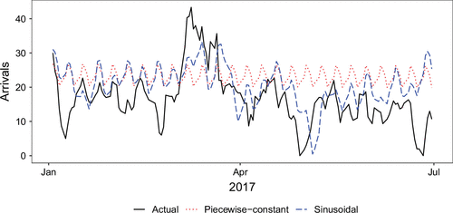
Note. The sinusoidal model and the piecewise constant one are fit to data from an earlier period, and their predictions for this period are displayed.
To more systematically contrast the performances of the sinusoidal and standard NHPP approaches, in Section 3, we use a naturalistic staffing simulation based on data from a bank call centre in the United States. The data provide enough resolution to identify the intraday variations in call volumes for staffing, and the arrival pattern is also aperiodic: In addition to a dominant weekly cycle, we also detect the existence of {15.2, 31.1, 93.3} day cycles in the arrival pattern. By varying the amplitudes of the nonweekly cycles in the simulation relative to the weekly one, we see that staffing decisions based on (1) progressively outperform the standard approach as the underlying arrival rate deviates from a weekly structure.
An example of a periodic arrival pattern comes from patient arrivals to an emergency department (ED) in the United States, which we will empirically show to be weekly periodic. For such arrivals, we expect both the sinusoidal and standard NHPP approaches to be comparable, matching what we see in the simulation study. However, in practice, it is rarely known a priori whether the arrival rate for a particular setting is periodic, let alone what the period is. In applications, the periodicity assumption is rarely checked beforehand. The simulation results demonstrate that it is important to first fit the sinusoidal NHPP to arrivals data in order to verify periodicity before proceeding further. Hence, (1) is still useful in this case.
After showing why managers should care about sinusoidal NHPPs, our second goal is to rigorously test the sinusoidal NHPP assumption in real-world settings. In Section 4, we develop an exact parametric bootstrap test for whether a given arrivals data set is generated from a sinusoidal NHPP. We use this test in Section 5 to obtain the first systematic evidence that the sinusoidal NHPP is consistent with data from two settings of great interest in service operations: patient arrivals to an emergency department and customer calls to a bank call centre. This is an important finding for the basic science of service systems, because it provides firm support for many existing queuing models that rely heavily on this previously untested assumption. Our finding provides the first rigorous justification for its use.
For researchers interested in applying the sinusoidal NHPP model, we include a description of the estimation procedure we use to fit (1) in Appendix A. The accompanying code can be found at www.github.com/rgurlek/sine-NHPP.
1.1. Related Work
A popular way to model NHPPs is to use a piecewise constant arrival rate function, for example, by averaging over arrival counts for Tuesdays, 10:00 a.m. to 11:00 a.m., over successive weeks. Although this approach can approximate any weekly periodic arrival rate arbitrarily well with small enough intervals, it is nonetheless discontinuous. For continuous rate functions, piecewise linear functions have been proposed (Massey et al. 1996, Zheng and Glynn 2017), and if some smoothness is also desired, cubic splines can be employed (Alizadeh et al. 2008).
However, arrival patterns occurring in the real world typically exhibit strong seasonal patterns, as can be seen in emergency departments (Zeltyn et al. 2011, Saghafian et al. 2012, Armony et al. 2015, Shi et al. 2015, Whitt and Zhang 2019). This naturally points to (1) as a candidate for the arrival process, which also comes with the benefit of being infinitely smooth. Although special forms of (1) are frequently assumed in analytic queuing models,2 until recently, it was challenging to fit (1) to data, which may have hindered its adoption in practice. This is because neither the number of frequencies (p) nor the frequencies themselves are assumed to be known in (1), making this an infinite-dimensional estimation problem. The problem was only recently solved in the statistical learning literature (Shao and Lii 2011, Chen et al. 2019). In this paper, we use a variant of the fitting procedure in Chen et al. (2019), which achieves the best possible frequency resolution.
Although this paper studies an NHPP arrival model that has a deterministic rate, we note that there is a stream of literature surveyed in Ibrahim et al. (2016) that treats the arrival process as an NHPP with a stochastic rate, that is, a Cox process. This can happen if depends on unobserved or stochastic variables, which will introduce additional uncertainty into the estimate of the rate. See the discussions in Jongbloed and Koole (2001), Steckley et al. (2005, 2009), Akşin et al. (2007), Bassamboo et al. (2010), Koçağa et al. (2015), Ibrahim (2018), Whitt and Zhang (2019), Sun and Liu (2021), and the references therein. These more complex models represent refinements of the NHPP and are suited to supporting decision making over short time scales, where recent information (e.g., today’s realized demand, weather forecast) can be used as variables to forecast demand for the near future.
Recently, a subclass of the Cox process called the Hawkes process has gained attention as a model for arrivals over even shorter time scales. In a Hawkes arrival process, an arrival increases the intensity of another arrival through self-excitation (Daw and Pender 2018, 2022; Gao and Zhu 2018; Daw et al. 2021). For example, Daw et al. (2021) studies a contact centre where customers chat over text with service representatives, and the arrival of messages from the customers is likely to “excite” the arrival of responses from the representatives. The time scale under consideration here is on the order of minutes, which makes for a novel high-frequency setting.
2. Implications of the Sinusoidal NHPP for Managing Service Systems
Even though the sinusoidal NHPP (1) is parsimonious and intuitively appealing, it may not be immediately obvious how it adds value to the management of service systems. The utilitarian manager may question why they should abandon existing NHPP models in favour of (1). In this section, we articulate how the sinusoidal NHPP model can be used to improve the performance of service systems, and in the next section, we back up our argument with results from a naturalistic simulation.
Specifically, we examine whether there are particular types of sinusoidal arrival patterns for which the use of (1) can improve the performance of service systems. The answer is of course relative to the other NHPP models currently in use, the most popular ones being piecewise constant or piecewise linear arrival rates (Massey et al. 1996, Zheng and Glynn 2017). Although these models are nonparametric and do not require the arrival rate to be periodic, the value of is unknown in practice and can only be estimated over some past time interval . To extrapolate into the future (t > T) for prescriptive use, inevitably one has to assume that repeats itself periodically, that is, for t > T. A period of one day or one week is commonly assumed in applications, but this is rarely verified empirically beforehand.
Hence, to use the existing arrival rate models for decision making, it is necessary to first assume that is periodic, and that its period is known to the decision maker. This insight suggests that we segment sinusoidal arrival patterns into two classes: periodic patterns and aperiodic ones.
2.1. Periodic Patterns
If the underlying arrival rate is periodic, then the sinusoidal NHPP offers no clear advantage over existing NHPPs, besides being infinitely smooth. This is because the latter can also approximate arbitrarily well over the duration of one period, if the length of the period is known. However, in reality, it is rarely known a priori whether the arrival rate for a particular setting is periodic, let alone what the period is. Hence, before applying existing NHPP models, managers should still first fit a sinusoidal NHPP to check whether the periodicity assumption is reasonable. If so, the period can then be inferred from the estimated frequencies. As an example, this is done in Section 5.1, where we verify that a weekly period is appropriate for the patient arrivals to an emergency department, in agreement with Whitt (2018).
2.2. Aperiodic Patterns
Suppose the frequencies identified by the fitted sinusoidal NHPP are not compatible with a weekly periodic structure. Using existing NHPPs would then lead to substantial biases if the amplitudes of the nonweekly cycles were sufficiently large, in which case the sinusoidal NHPP would outperform. We saw an example of this in Section 1 regarding customer calls to a Turkish car dealership. A description of the data set and the analysis can be found in Appendix B. Customer calls to the bank call centre that we study in Section 5.2 are another example of aperiodic arrivals: For one of the major customer classes, called Voice Response Unit (VRU)-Premier, we identify three cycles (15.2, 31.1, and 93.3 days) from the data that do not fit with the rest of the week-based cycles.
To recap, the sinusoidal NHPP model is necessary and valuable in either scenario. For the first case, it serves as a spectral technique for verifying and estimating the periodicity of the arrival pattern. As such, it complements rather than competes with existing NHPP models. For the second case, it directly serves as the arrival model to use for prescriptive planning. Via the use of naturalistic simulations, in the next section, we illustrate the possible performance gains from using the sinusoidal NHPP to staff service systems driven by aperiodic customer arrivals.
3. Performance of Staffing Policies Based on Sinusoidal NHPP Models
We construct a sequence of naturalistic staffing simulations for the bank call centre we will empirically study in Section 5.2. We focus on the VRU-Premier customer class, whose call pattern exhibits nonweekly cycles. (Table 3 lists all the frequencies identified from the data.) The simulations allow us to see how the performance of the sinusoidal NHPP varies as the underlying arrival pattern deviates from a weekly periodic structure. This is achieved by gradually increasing the amplitudes of the nonweekly cycles relative to the week-based ones.3
3.1. Arrival Model
The arrival rate functions used to generate the simulations are piecewise constant and inherit the cycles estimated for the VRU-Premier class: a week-based cycle, a 15.2-day cycle, a 31.1-day cycle, and a 93.3-day cycle. We specify a family of arrival rates indexed by as
The week-based fixed effects for each of the 30-minute subintervals of a week. The width of the subintervals are approximately how often staffing levels are adjusted in call centres (Dietz 2011).
The fixed effects for the 15.2-day cycle, broken into 10 piecewise constant subintervals of equal width, and and follow the same approach for the 31.1-day cycle and the 93.3-day cycle, respectively. Having more subintervals allows us to better reproduce the exact cycle, but the piecewise constant ground truth will also converge toward a smooth cyclic one. This would give the sinusoidal NHPP an increasing advantage.
The constant is set as the smallest one that ensures . Given that it is constant, it plays no role in determining the seasonality of the arrivals.
For our purpose of investigating how the cycles in the arrival pattern affect the relative performance of staffing policies based on the sinusoidal NHPP, the trend is of ancillary interest and is excluded from (2).4 The values of the seasonal fixed effects , and are estimated in the following way. First, the arrivals in the VRU-Premier data are aggregated into 30-minute subintervals, where yt is the count for the subinterval that begins at time hours for . These are then regressed onto dummies for the seasonal effects and also an intercept and a linear trend. Only the seasonal effects are used in (2).
When α = 0, the arrival rate (2) is purely weekly periodic. A weekly periodic piecewise constant model that is fit to arrivals data generated from should then perform the best. However, as α grows, the nonweekly cycles will come to dominate, so the sinusoidal NHPP should perform better.
3.2. Simulation Model
We first model the call centre as an queue where customer calls arrive according to . The staffing level at time t is st, which can be adjusted every 30 minutes. From the data, we estimate the exponential service rate to be 18.6 customers per hour per agent. As a second model, we allow for a completely general service time distribution, that is, , as a contrast to the simple exponential one in the first model. The distribution for the general service time is estimated from the empirical distribution of the call durations. Although it is possible to also add customer abandonment to the model, as is done in the analysis of the dealership data (Appendix B), the results there suggest that our qualitative findings would not change as α increases.
For each model and for each , we generate call arrivals and service times over 12 months to use as the in-sample period, and also generate a 13th month as the test period. This is in line with the empirical analysis of the bank call centre data in Section 5.2, where the sinusoidal NHPP is fit to data from April 2001 to March 2002, and April 2002 is held out as the test period. The simulated in-sample period is used to fit three competing NHPP models to use for planning staffing levels for the test period:
Weekly PC: The arrival rate is piecewise constant over each of the 168 hours of the week. The weekly period is a typical assumption in applications where spectral methods are not used beforehand to inspect the frequencies in the arrival pattern. Note that the ground truth (2) is also piecewise constant.
Monthly PC: The arrival rate pattern is piecewise constant and repeats every 30 days. The model employs the same number of intervals as Weekly PC, but is based on a 30-day period rather than a 7-day one.
Sine: This is the sinusoidal NHPP (1).
3.3. Staffing Policies
Staffing decisions for the test period depend not only on the arrival and service rates fitted to the in-sample period, but also on the manager’s objective. We consider two commonly used objectives:
Delay: The probability that an arriving customer has to wait before receiving service is
where Nt is the number of customers currently in the system. The manager’s problem is to find the smallest st subject to the constraint that the delay probability is below a prespecified threshold. A 20% threshold is used in this study.Cost: The expected cost of staffing plus customer waiting cost is
The manager’s problem is to choose st to minimize this. The waiting cost = $70.5/hour is based on the one for high-priority customers of an Israeli bank call centre in 2008 (Akşin et al. 2013), but adjusted to 2021 U.S. salary levels. The agent staffing cost = $15.7/hour is taken from the average 2004 U.S. call centre salary figure in Hillmer et al. (2004), adjusted to 2021 dollars.
Our goal is not to develop optimal staffing policies under each objective. Rather, we aim to compare the performances of the arrival models under a widely used staffing rule called the modified-offered-load (MOL) approximation as described in Feldman et al. (2008). We use the MOL approximation to set st for each 30-minute interval in the test period. In the context of an queue, the MOL approach first calculates the mean number of busy servers, , for the infinite server version of the queue, that is, . The term has a closed-form expression, and we use its maximum value inside an interval as the offered load for the finite-server queue. The stationary distribution of this queue is then used to solve for the manager’s problem to obtain st.
3.4. Results
Tables 1 and 2 display the performance of using the PC and Sine models fits to staff the call center during the test period, for the and models, respectively. Before delving into the results, note that the PC models share the same piecewise constant structure as the ground truth (2) used to generate the data. This gives the Weekly PC model an unfair advantage especially when α = 0, because in this case, its weekly period is also correctly specified for the underlying arrival rate.
|

Table 1. Performances Under the Ground Truth
| α | Delays in excess of 20% | Daily cost | ||||
|---|---|---|---|---|---|---|
| Sine (%) | Weekly PC (%) | Monthly PC (%) | Sine (baseline) ($) | Weekly PC ($) | Monthly PC ($) | |
| 0 | 0.0% | 0.0 | 15a | 6,520 | 6,500b | 12,760b |
| 1 | 0.0% | 0.0 | 20a | 6,680 | 6,710b | 15,930b |
| 2 | 0.0% | 3.3a | 24a | 6,800 | 7,080b | 18,520b |
| 3 | 0.0% | 10a | 31a | 7,010 | 8,330b | 25,590b |
Note. The lowest cost is in bold.
aDelay probability exceeds 20% by more than three standard errors (based on 100 replications of the test period).
bMean difference in costs is more than three standard errors away from zero.
|
Table 2. Performances Under the Ground Truth
| α | Delays in excess of 20% | Daily cost | ||
|---|---|---|---|---|
| Sine (%) | Weekly PC (%) | Sine (baseline) ($) | Weekly PC ($) | |
| 0 | 0.0 | 0.0 | 6,480 | 6,450b |
| 1 | 0.0 | 0.0 | 6,620 | 6,630b |
| 2 | 0.0 | 4.1a | 6,750 | 7,010b |
| 3 | 0.0 | 9.3a | 6,930 | 7,650b |
Note. The lowest cost is in bold.
aDelay probability exceeds 20% by more than three standard errors (based on 100 replications of the test period).
bMean difference in costs is more than three standard errors away from zero.
For the staffing policies driven by the delay objective, we first calculate the percentages of customers who had to wait during the test period, Pwait, and then report the amounts in excess of 20% in the left columns of the tables:
If this is zero, then the staffing policy achieves the intended goal of capping the proportion of customers who have to wait to 20%. Focusing on the results for the ground truth first (Table 1), we see that the staffing policy based on the Sine model achieves the delay target for all values of α, whereas the staffing policy based on the Weekly PC model fails as the nonweekly cycles grow with α. For example, when α = 3, the proportion of customers who have to wait is under the ground truth, which is 50% higher than the cap. Even worse, the Monthly PC model misses the delay target by 15 percentage points even when α = 0.
For the staffing policies driven by the cost objective, we report the average daily costs realized during the test period in the right columns of the tables. Once again focusing first on Table 1, we see that Sine staffing always performs better than Weekly PC staffing, except for the weekly periodic case (α = 0). We observe cost savings of up to 19% as the nonweekly cycles grow with α. As mentioned earlier, the Weekly PC model enjoys an unfair advantage over the Sine model when α = 0. Despite this, Sine staffing is less than 0.5% more costly in this case. Monthly PC staffing performs the worst of the three, with costs that are two to three times higher than those incurred under Sine staffing.
The poor performance of the Monthly PC model even at α = 0 (when only a weekly cycle exists) is due to the fact that it is unable to adapt to the seven-day cycle, because 30 is not a multiple of seven. The performance is further exacerbated by the other nonmonthly cycles as α grows. With this understanding, it suffices to focus on the Weekly PC benchmark for the simulation based on the ground truth (Table 2). We see that the situation is essentially the same as in the case for . Thus, whether we assume exponential or general service times, Sine staffing always performs better than Weekly PC staffing, except for the weekly periodic case (α = 0).
Putting the results together, we see as expected that the sinusoidal NHPP outperforms when the arrival pattern deviates from a periodic structure. This finding is robust to the service time distribution employed, from the simple exponential to completely general ones. Applications that employ existing NHPP models implicitly assume that the arrival pattern is periodic, but this assumption is rarely tested beforehand. Our results demonstrate that failing to do so can lead to significant performance losses.
4. Testing for Sinusoidal NHPPs
Having provided arguments for why managers should care about the sinusoidal NHPP (1), before employing them, we still have to first verify that it is in fact a reasonable model for real-world arrivals. Given customer arrival timestamps generated from an arrival process in the observation window , we develop a statistical test for whether is a sinusoidal NHPP. Specifically, the null hypothesis of interest is
Note that this is more stringent than the null hypothesis tested in Brown et al. (2005) and Kim and Whitt (2014a),
On the other hand, tests based on the sharper null , such as the one we develop here, go one step further to pin down the functional form of the arrival rate function. To do this, we first need an estimate of the sinusoidal rate function. Given that a fitting procedure did not exist until recently, this may explain the lack of work on validating the sinusoidal NHPP to date.
4.1. Fitting Sinusoidal NHPPs
Fitting the sinusoidal NHPP (1) is more complicated than fitting the special case of the truncated Fourier series model in Eick et al. (1993). In the latter, the frequencies are prespecified, so the amplitudes and phases can be estimated using (complex-valued) linear regression. The more flexible case (1) allows the frequencies to be free, so they also need to be estimated from data as well. Appendix C provides a stunning counterexample showing how standard spectral methods can fail at this.
Fortunately, the statistical learning technique introduced in Chen et al. (2019) is able to provably recover (1) if the underlying arrival process is indeed a sinusoidal NHPP. However, the approach uses a thresholding step that is not trivial to apply. In Appendix A, we introduce a simpler variant that works well in practice (Algorithm A.1), with code provided on GitHub (www.github.com/rgurlek/sine-NHPP). This is the method that will be used in this paper, and is also the approach we recommend to managers of service systems.
4.2. The Statistical Test
Given a consistent estimate of the sinusoidal arrival rate, we divide the arrivals window into subintervals and test the null within each subinterval. Because no model is perfect, we do not expect the parsimonious sinusoidal NHPP model to fit well to all subintervals. Therefore, if it passes a goodness-of-fit test for a large majority of subintervals, then we deem it to be a reasonable model. We first propose a test for a single time interval, and then describe multiple testing corrections for applying the test to all subintervals.
4.2.1. Single Subinterval.
Consider testing for the arrival process generating the arrivals in an interval .5 We use the time-change property of NHPPs as articulated in Proposition 1 below to develop an exact parametric bootstrap test that applies to an NHPP with a given hypothesized arrival rate function. This differs from the test in Brown et al. (2005) and Kim and Whitt (2014a), which is based on the conditional uniform property of homogeneous Poisson processes. Their test does not specify a particular functional form for the arrival rate of the NHPP, so they use a Poisson process with a constant rate to locally approximate the unknown arrival rate over small time subintervals. This results in a nonexact test that requires the subinterval widths to shrink at an appropriate rate for it to be asymptotically valid.
The arrivals follow an NHPP with rate (1) and cumulative rate if and only if
It follows that if the distribution of deviates significantly from uniformity, we should reject the null that come from an NHPP with rate . One possible test for this is to use the Kolmogorov–Smirnov statistic
In practice, substituting the estimated for means that the null hypothesis we are actually testing is that the arrival process is an NHPP with the particular sinusoidal rate . Note that this even more stringent than , which is to test whether the NHPP rate function follows any sinusoidal pattern at all.
4.2.2. All Subintervals.
If each subinterval is of length L, then applying the test above to each subinterval will yield T/L hypothesis tests. A multiple testing correction is then needed to control the number of false rejections at the 5% level. For a single test (i.e., ), this corresponds to controlling the type I error, and a generalization of the type I error to multiple tests is the familywise error rate
To see why it is not enough to just control the type I error of each individual test (i.e., reject a test whenever its p-value is less than 0.05), suppose for simplicity that we have 10 independent tests, and that all null hypotheses are true. Thus, the probability that each test results in a false rejection is 0.05, but the probability that there is at least one false rejection among the tests is .
We will use the procedure of Holm (1979) to ensure that . The procedure is uniformly more powerful than the better-known Bonferroni correction, and works in the following way: Let be the ordered p-values from the smallest to the largest, and compute the smallest k such that
The null hypotheses associated with are then rejected, whereas the ones associated with the larger p-values are not.
Note that the FWE is the probability that any of the rejected nulls is a false rejection, so it can be very hard to control when there are a large number of tests. A popular alternative is to control the false discovery rate
5. Validating the Sinusoidal NHPP in Real-World Settings
Armed with the statistical test developed in Section 4 for assessing the sinusoidal NHPP assumption, we now analyze arrivals data from two settings of great interest to the service operations community: patient arrivals to an emergency department and customer calls to a bank call centre. Our results provide empirical support for the sinusoidal NHPP assumption, but in general, each new setting should be validated before use. The analysis we follow here can serve as a template for testing those settings as well.
5.1. ED Patient Arrivals
We analyze a data set from the ED of a U.S. academic hospital containing timestamps for 168,392 patient arrivals from 2014 to third quarter (Q3) of 2015 (T = 652 days). In addition, the Emergency Severity Index (ESI) of each patient is also recorded, with level 1 being the most severe (e.g., cardiac arrest) and level 5 the least (e.g., rash). Information on demand for ED services is a critical input to staffing and other operational decisions that influence the efficiency of healthcare delivery, and it enables the construction of high-resolution queuing simulations. For the ED in question, ESI level 1 trauma patients ( of arrivals) are assigned to dedicated bedspaces on arrival and are therefore excluded from the analysis.
ESI level 2 patients are treated in a ward separate from the other ESI levels, so from a capacity management perspective, we will analyze this group on its own. Previously, Chen et al. (2019) fitted a sinusoidal rate for this group using their technique, and visually compared the fit to the empirical average rate for each hour of the week. Such a cursory analysis is, however, far from complete, because the arrival rate itself tells us nothing about the statistical process of the arrivals: The fitted rate can be consistent with a Cox process with a mean rate that is sinusoidal, and it can even be consistent with a deterministic arrival process. Here, we systematically analyze the data to determine whether the arrival data come from a sinusoidal NHPP.
ESI level 3 to level 5 arrivals are not only distinct from level 2 from a capacity management standpoint, they are also behaviourally different in a way that can potentially violate the NHPP property. Whereas level 2 patients require immediate care from the time illness occurs, lower-acuity patients belonging to levels 3 to 5 often have flexibility to delay seeking treatment. Thus, even if the occurrence of illness among these patients follows an NHPP, the flexibility to postpone treatment may result in non-NHPP arrivals to the ED. Indeed, our analysis suggests that low-acuity cases may delay seeking treatment going into the weekend, resulting in a spike in visit volume on Monday. Therefore, it is necessary to analyze this group independently of ESI level 2.
5.1.1. ESI Level 2.
A total of 66,240 patient arrivals were assigned an ESI level of 2. As shown in the left panel of Figure 2, our fitting procedure (Algorithm A.1 in Appendix A) selected four intraday frequencies and six week-based ones. The intraday frequencies include a daily cycle (), a 12-hour cycle (), an 8-hour cycle (), and a 6-hour one (). The week-based cycles include a 1-week cycle (), a 1/2-week cycle (), a 1/3-week cycle (), a 1/5-week cycle (), a 1/6-week cycle (), and a 1/8-week cycle ().
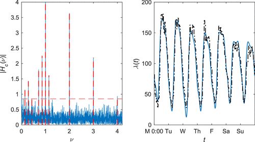
Notes. The left panel shows the centralized windowed periodogram ((A.3) in Appendix A). The selected threshold is represented by the dashed horizontal line, and the location of the frequency estimates are given by the vertical ones. In the right panel, the estimated arrival rate (arrivals per day) over the course of a week is given by the solid line. The dashed and dotted line represents the empirical average arrival rate for each hour of the week.
Given that the fitted rate has a weekly period, we can compare it to the empirical average arrival rate for each hour of the week (right panel of Figure 2). The estimate reveals two intraday peaks, the first at around 11:00 a.m. and the second at around 5:00 p.m. We also see that the intensity of arrivals fades steadily into the weekend. For most parts of the week, the sinusoidal fit does a very good job capturing the variation in the empirical arrival rate, at least from a visual standpoint.
To use the statistical tests from Section 4 to rigorously quantify the goodness of fit of a sinusoidal NHPP, we divide the arrival data into time subintervals of length L = 2 hours. Of the resulting subintervals, the null hypotheses for only 7% of them are rejected, and this is before applying any multiple testing corrections (which will reject even fewer hypotheses). Hence, the sinusoidal NHPP is a reasonable model for ESI level 2 arrivals.
5.1.2. ESI Levels 3 to 5.
There were in aggregate 99,205 arrivals assigned to ESI levels 3 to 5. Figure 3 shows that three of the intraday frequencies from the level 2 case are selected (the six-hour cycle is now absent), and only the 1/5- and 1/6-week cycles are selected from the week-based ones. The estimated arrival rate exhibits a more subdued day-of-week effect when compared with level 2, but the midday peak is now more pronounced relative to the evening one. We know from Fourier theory that capturing these time-localized effects will require more sine waves than the sparse specification (1) is designed for, which explains the sinusoidal model’s underfit to the large peaks early on in the week. Interestingly, the peaks drop from Thursday on as the weekend approaches, and culminates in a substantial spike in arrivals on Monday. As alluded to earlier, this could be related to the fact that low-acuity patients have flexibility in deciding when to seek treatment. Future research should look into the behavioural mechanisms behind this pattern.
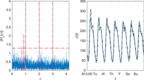
Notes. The left panel shows the centralized windowed periodogram, selected threshold, and locations of the frequency estimates . The right panel shows the estimated (solid line) and empirical (dashed and dotted line) arrival rates over the course of a week.
Despite this potential complication, only 8% of the 7,824 subintervals are rejected, just slightly more than for level 2 arrivals. Thus, the sinusoidal NHPP remains a good model for ESI level 3–5 arrivals.
5.1.3. Seasonal Effects.
No year-based seasonal cycles (365/12 (monthly), 365/4 (quarterly), 365/2, 365) are selected from the data. As explained in Appendix A, our fitting procedure cannot resolve frequencies that are within cycles/day of each other, so it is possible that we missed cycles larger than days, that is, the semiannual and annual cycles. To see whether these cycles actually exist in the data, we add them to the set of frequencies selected by our procedure and reestimate the amplitudes of the cycles. For both ESI groups, we find that the semiannual cycle is negligible, and that the annual cycle is weaker than the weakest frequency signal selected by our procedure. For example, for ESI levels 3 to 5, the amplitudes of the selected frequencies range from 4.0 to 44. The amplitudes of the semiannual and annual cycles are 0.82 and 3.3, respectively. Thus, our finding is consistent with Whitt (2018), which argues that a week is the natural period to use in healthcare settings.
5.2. Customer Calls to a Bank Call Centre
The call data come from a bank in the United States, and were kindly made available by the SEELab at Technion (Mandelbaum 2017). The bank’s call centre consists of sites across the Northeast that are integrated into one virtual centre. About a fifth of the callers seek to speak with a live agent, whereas the rest conduct self-service transactions at the VRU, Announcement, or Message stages. Kim and Whitt (2014a, section 5.4) studies whether the call arrivals between 7:00 a.m. and 10:00 p.m. in the 30 days of April 2001 can be modelled by NHPPs. Among the eight call types in the data, six are found to pass the NHPP test in more than 75% of days. These call types are VRU-Premier, VRU-Business, VRU-Loan, VRU-Summit, Business, and Message.
To further test whether arrivals from these call types can be modelled by a sinusoidal NHPP, we use calls arriving between April 2001 and March 2002 inclusive to fit the arrival rate, and hold out April 2002 as the test period. Arrivals of the type VRU-Summit appeared in only 140 days of record during the period (up until August 2001); therefore, we consider only the other five types of calls.
Table 3 shows the 21 frequencies selected by our fitting procedure for the arrival rate of VRU-Premier calls. In addition to the intraday and the week-based cycles, frequencies with periods of 15.2 days, 31.1 days, and 93.3 days are also selected. Because these do not divide seven evenly, the arrival rate for a specific hour of a particular day of week will vary from week to week, making it impossible to plot the empirical arrival rates over the course of a week like those in Figures 2 and 3. The deviation from a weekly structure may also explain a portion of the overdispersion discovered in Kim and Whitt (2014a).
|
Table 3. Frequencies Selected for the Arrival Rate of VRU-Premier Calls
| # cycles per day | # cycles per week | Other cycles |
|---|---|---|
| 1 to 4 | 1 to 6, 8 to 13, 15, 20 | 1 cycle per 15.2 days |
| 1 cycle per 31.1 days | ||
| 1 cycle per 93.3 days |
The first column of Table 4 displays the number of calls of each type from April 2001 to March 2002 inclusive. We see that VRU-Loan has the lightest call volume, but on a per unit time basis, even this has roughly four times as many arrivals as ESI levels 3–5 in Section 5.1. This allows us to use 30-minute subintervals for the statistical tests in Section 4, which is approximately how often staffing levels are adjusted in call centres (Dietz 2011). The last two columns of Table 4 show the results of applying the tests to the April 2001 period studied in Kim and Whitt (2014a). Whether we correct for multiple testing issues using FWE or FDR, we see that the null hypotheses for most of the subintervals are not rejected. Applying the tests to call arrivals in the April 2002 test period yields similar results (Table 5). Taken together, our results build on the finding in Kim and Whitt (2014a) by further showing that the sinusoidal NHPP is a reasonable model for NHPP call types.
|
Table 4. In-Sample Results from Applying the Tests in Section 4 to Calls to the Bank in April 2001
| # calls btwn April 2001 and March 2002 | # calls in April 2001 | % subintervals not rejected | ||
|---|---|---|---|---|
| (%) | (%) | |||
| VRU-Premier | 1,071,481 | 96,187 | 97 | 98 |
| VRU-Business | 2,571,511 | 218,163 | 83 | 90 |
| VRU-Loan | 208,328 | 13,782 | 99 | 99 |
| Business | 987,606 | 71,010 | 84 | 91 |
| Message | 977,579 | 78,914 | 85 | 90 |
Note. Thirty-minute subintervals are used to group calls between 7:00 a.m. and 10:00 p.m., resulting in a total of 900 subintervals.
|
Table 5. Results from Applying the Tests in Section 4 to Calls to the Bank in the April 2002 Test Period
| # calls in April 2002 | % subintervals not rejected | ||
|---|---|---|---|
| (%) | (%) | ||
| VRU-Premier | 98,910 | 97 | 98 |
| VRU-Business | 225,862 | 77 | 86 |
| VRU-Loan | 16,610 | 99 | 99 |
| Business | 88,988 | 86 | 90 |
| Message | 101,619 | 70 | 80 |
Note. Thirty-minute subintervals are used to group calls between 7:00 a.m. and 10:00 p.m., resulting in a total of 900 subintervals.
6. Discussion
Special forms of the sinusoidal NHPP (1) have long been employed in the queuing literature. This is the first paper to systematically validate the model as a reasonable one for arrival processes of interest in service operations, providing firm support for the many existing queuing models that rely heavily on this previously untested assumption. From a prescriptive viewpoint, our work clarifies how the sinusoidal NHPP can be used to improve the performance of service systems. Our simulation results highlight the importance of first verifying the periodicities in the arrivals data before imposing a periodic structure on the fitted arrival rate function.
Given the simplicity and tractability of the sinusoidal NHPP, we hope our findings will spur more interest in its practical adoption. In turn, we hope this will encourage queuing theorists to revisit the sinusoidal NHPP as a workhorse model for time-varying arrivals. Such efforts could generate further analytical results that add to the existing ones for sinusoidal arrival rates (Eick et al. 1993, Feldman et al. 2008, Liu and Whitt 2012), potentially leading to a virtuous cycle where theory advances practice and vice versa.
The ED arrivals data were kindly provided by Dr. Kito Lord. The authors also grateful to Noa Zychlinski and the SEELab at Technion for providing us with access to the call centre arrivals data. The authors are grateful to the review team for providing many insightful suggestions that improved the exposition and analyses in this paper.
Appendix A. Estimation Procedure for Fitting (1)
Here we introduce a simpler variant of the estimation procedure in Chen et al. (2019) that works well in practice. Code for implementing this can be found at www.github.com/rgurlek/sine-NHPP. Before diving into the details of the estimation, there are two considerations that researchers interested in deploying sinusoidal NHPPs should be aware of.
First, the frequencies in (1) cannot be too close to each other, for otherwise it would be impossible to distinguish between them in a noisy setting. It suffices for the frequencies to be spaced apart from one another by more than . To make things concrete, we assume this gap is . In finite samples, our procedure also requires the gap between frequencies to be sufficiently positive, that is, no smaller than :
Second, the precision of the frequency estimates need to be sharper than in order to obtain consistent estimates for itself, that is,
Unlike (A.1), this is a property required of the estimation procedure, rather than an assumption imposed on the arrival rate. Note that (A.2) is stronger than consistency of the frequency estimates, which requires only a precision of . In Appendix C, we present a spectacular real-life example to show how standard spectral techniques can fail to achieve (A.2), and hence lead to disastrously wrong estimates for .
To provide intuition for our estimation approach under the frequency resolution (A.1), the frequency components of the arrival process consists of mixed in with the frequency components of statistical noise. This is because we can decompose the arrival process into its Doob–Meyer form,
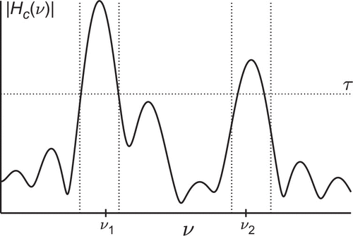
Notes. In the depicted periodogram, there are two signal frequencies, ν1 and ν2. Setting τ (horizontal line) above the ambient noise level leaves behind two bands (between the pairs of vertical lines) that contain ν1 and ν2.
Although there exists a theoretically justified bound for τ, in practice, the noise level can often be eyeballed from the power spectrum plot; see, for example, Figures 2 and 3. Hence, we will select τ by visual inspection instead. We verified that this yields essentially the same arrival rate fits in our empirical analyses, showing that this simpler approach is effective in practice. This is to be expected, because only frequencies with small amplitudes (on par with the noise level) might be missed this way, whereas the overall arrival rate fit is driven by the dominant frequencies.
The estimation procedure is described in Algorithm A.1. We make two remarks. First, the frequency components of N(t) can be visualized using a periodogram, which plots the frequency amplitudes against the frequencies (see Figure A.1). Algorithm A.1 uses the centralized and windowed periodogram
Chen et al. (2019) shows that their technique will consistently recover the sinusoidal NHPP (1) if, informally, the ratio of the largest to the smallest amplitude is less than 14.5. This can, however, be greatly relaxed. For example, if the constant four appearing in the frequency gap (A.1) is relaxed to six, then the maximum allowable ratio can be increased to over 100, provided that we replace the window in (A.3) with and substitute in Step 2 of Algorithm A.1. Given that Algorithm A.1 is the same as in Chen et al. (2019) save for the choice of τ, we also expect consistent recovery under the same conditions. If theoretical guarantees for the estimation procedure are absolutely required for a particular application, then the threshold used in Chen et al. (2019) can always be used.
(Procedure for Fitting (1))
1 Graph the periodogram defined in (A.3) over the range of frequencies of interest.
2 Set and visually estimate the noise level τ from the periodogram.
3 Identify the frequency region where the value of periodogram exceeds τ.
4 Set , k = 1 and repeat the following steps:
• Find the highest stationary peak of the periodogram in R and set as the corresponding frequency location. If no peaks exist, then exit loop.
• Perform the updates and . This removes a neighbourhood of radius r centred at from R.
5 and are given by the moduli and phases of the entries of the complex-valued vector , where the (j, k)-entry of the matrix is
and the kth entry of the -vector y is .
Appendix B. Customer Calls to a Car Dealership
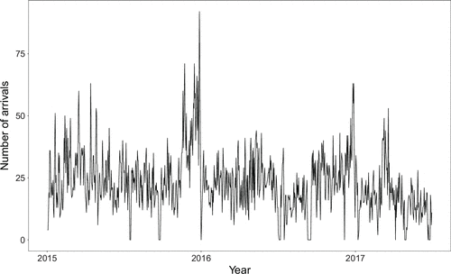
These data consist of daily customer call volumes for a car dealership in Turkey from January 2015 to June 2017, inclusive, with the first two years set aside as the in-sample period, and H1 2017 reserved for the test period. Each arrival is a phone call by a potential customer, and they are served by one of the sales staff between the business hours of 8:30 a.m. and 6:30 p.m., six days a week (closed Sundays). As a result, we will operate under a six-day week. The mean and median numbers of calls received per day are 19.1 and 18, respectively, with a high of 92. The arrival pattern over the entire period is given in Figure B.1. We see strong seasonal patterns that extend well beyond the weekly time frame, driven possibly by the timings of incentive programs and multiyear model refresh cycles.
Fitting Sine and PC Arrival Models
We fit the Sine and PC models from Section 3 to the in-sample period of the dealership data. The fitted models are then used to plan staffing for the test period.
In contrast to the ED and bank call centre data, where we observe the exact times of the calls, the dealership data report only the aggregate number of calls per day. For these discretized data, the statistical methods for the former settings are not applicable, so to estimate the periodicities for the Sine model, we use discrete Fourier transform. The counterexample in Appendix C shows that this is suboptimal for estimating frequencies from bucketed arrivals data, so the performances we report here for the sinusoidal NHPP likely underestimate its true performance.
Specifically, for the PC model, we regress the daily arrival counts onto a linear trend as well as dummies for the six business days of the week for the dealership. The fitted PC daily arrival rate for day t is then given by the coefficient for the day of the week for t plus the trend effect. For the Sine model, we estimate the frequencies of the arrival pattern by applying discrete Fourier transform to the centered and detrended daily arrival counts.6 The amplitudes and phases for the identified cycles are then estimated by regression jointly with the intercept and the linear trend. Table B.1 ranks the estimated cycles by amplitude.
|
Table B.1. Cycles Identified from the Dealership Data
| Cycle (in calendar days) | Amplitude |
|---|---|
| 338 | 4.47 |
| 7.00 | 4.37 |
| 195 | 4.11 |
| 153 | 4.00 |
| 3.50 | 3.62 |
| 34.3 | 3.23 |
| 74.5 | 2.78 |
| 30.6 | 2.39 |
| 15.2 | 2.38 |
| 94.4 | 2.24 |
| 60.7 | 2.09 |
| 14.2 | 2.00 |
| 9.84 | 1.91 |
| 12.2 | 1.87 |
| 23.4 | 1.85 |
| 25.3 | 1.84 |
| 40.1 | 1.76 |
| 11.4 | 1.55 |
| 2.33 | 1.50 |
| 16.8 | 1.41 |
| 6.92 | 1.17 |
Note. The length of the cycle is scaled so that a seven-day cycle contains six business days for the dealership.
Staffing in Test Period
To evaluate the operational performances of Sine and PC models for staffing, note that we cannot plan staffing at an intraday resolution as in Section 3, because the intraday variation in arrivals cannot be identified from the aggregated data. Hence we consider a setup where the staffing level is set just once a day. This turns out to coincide with the dealership’s staffing policy: If an employee is staffed to work on a particular day, they work for the whole day.
For day t in the test period, we model the system as an (Erlang A) queue. Brown et al. (2005, p. 47) demonstrates how theoretical rules implied by this model “hold with reasonable precision” in the real world. The objective is to choose the staffing level st for day t in order to minimize the sum of labor cost and expected customer abandonment cost for that day, that is,
Here, csalary = 230 Turkish lira (TL) is the daily wage for the dealership, is the daily arrival rate, is the conditional steady-state probability of customers leaving the system without being served, is the sales conversion rate estimated by the manager, and TL is the estimated average profit from a sale (including after-sales services). The average service and patience times are 60 minutes and 10 minutes, respectively. The probability is estimated using the equation presented in Mandelbaum and Zeltyn (2009).
Hence, given a predicted daily arrival rate (from either Sine or PC) for day t in the test period, the prescribed staffing level is . Its performance is evaluated by , where Nt is the actual number of arrivals on day t. Averaging this over the days in the test period produces an overall performance measure for Sine or PC. We see from Table B.2 that Sine incurs significantly lower cost, in line with Figure 1, which shows that Sine also produces superior predictions for call volumes in the test period.
|
Table B.2. Comparison of NHPP Models for Setting Staffing Levels in the Test Period H1 2017
| Mean daily cost ($) | Excess over Sine (95% CI) | |
|---|---|---|
| Sine | 1,662 | |
| PC | 1,821 | 9.6% (6.7%, 12.5%) |
Note. CI, Confidence interval.
Appendix C. Counterexample Illustrating Why the Level of Frequency Estimation Precision (A.2) Is Needed
We consider a subset of 66,240 patient arrivals to an academic emergency department in the Unites States from 2014 to Q3 of 2015 (T = 652 days of observations). This subset corresponds to patients who are assigned ESI level 2, a measure of emergency severity. The data come from a capacity planning project for the emergency department, and to model patient demand, we fit the sinusoidal NHPP to it. We initially employed a standard discrete Fourier transform to estimate the periodicities in the arrival pattern. This requires bucketing the arrivals into discrete time bins, and the mean bin count in bucket is

Note. In the left panel, eight dominant frequencies stand out, the largest one being 1.0015 cycles/day.
To fit (1) using just these eight cosines, we reestimate their amplitudes ck and phases using least squares. The red dashed line in the right panel of Figure C.1 shows the resulting fit over the course of a Wednesday. Compared with the solid line representing the average hourly arrival count, the estimated arrival rate is essentially flat and completely fails to capture the intraday variation in arrivals. It is surprising that using an approach as standard as the discrete Fourier transform would lead to such discrepancies.
In this example, one might guess that the dominant frequency 1.0015 cycles/day is really just a noisy estimate of the daily cycle. Suppose we refit (1) to the seven other frequencies in addition to the daily cycle, that is, we replace 1.0015 cycles/day with 1 cycle/day and keep all other frequencies the same. The blue dotted line in Figure C.1 shows the resulting fit, which is a significant improvement over the previous one. This suggests that the frequency estimation error of 0.0015, which is in this case, is too large. In fact, replacing with a slightly more precise estimate of the daily cycle, say, , already provides a much more sensible fit (green dashed and dotted line).
Why?
The amplitude estimation involves regressing the arrival counts onto the explanatory variables , where are the estimated frequencies. Because, in this case, is likely a noisy estimate of , using as an explanatory variable in lieu of would result in model misspecification. For example, at time , the bias
Although Rice and Rosenblatt (1988) were the first to show that (A.2) is theoretically necessary for ordinary time series, to our knowledge, this is the first real arrivals example to show that the issue actually matters in practice, and is not just a mathematical pathology.
In this particular, case one might argue that 1.0015 cycles/day is clearly a noisy estimate for the daily cycle, so the analysis above is unnecessary. However, in general, the “obvious true” frequency may be wrong if the frequency estimate is, say, 1.93 cycles/day: As recounted in Parker (2011), the Allies’ planning of the Normandy landings hinged on understanding the periodicities in tidal heights, which represent the arrival rate of fluid parcels. In a prescient act of patriotism, P. S. Laplace demonstrated mathematically in 1776 that the dominant frequencies are 1.93 cycles/day and 2.00 cycles/day. Without this, the Allies would have had to determine the frequencies empirically instead, and mistakenly rounding 1.93 to 2 might well have changed the course of history.
1 If the arrival rate takes on the form of (1), then closed-form expressions for certain performance outcomes can be derived for , and queues (Eick et al. 1993, Feldman et al. 2008, Liu and Whitt 2012, Liu 2018).
2 See Green and Kolesar (1991), Eick et al. (1993), Jennings et al. (1996), Green et al. (2001), Feldman et al. (2008), Liu and Whitt (2012), Whitt (2014, 2016), Chan et al. (2016), and Liu (2018).
3 Unlike the bank call centre data, where we observe the exact times of the calls, the Turkish dealership data come aggregated at a daily level, so they cannot be used to set staffing at an intraday resolution. Using an alternate setup where staffing is fixed for each day, in Appendix B, we show that staffing with the sinusoidal NHPP also leads to better performance in the test period.
4 It is straightforward to incorporate trends in the sinusoidal and existing NHPP models, as is done for the dealership data in Appendix B. The sinusoidal NHPP remains superior in this setting.
5 Arrival times that have been rounded (e.g., to the nearest second) will require unrounding to remove interarrival times of zero if multiple arrivals are rounded to the same second. We follow Brown et al. (2005) and Kim and Whitt (2014a) in adding uniform random numbers between seconds to the timestamps to mitigate the problem.
6 A fine frequency grid is employed, which can be achieved by padding the vector of daily counts with zeroes so that the resulting vector contains 100,000 entries.
References
- (2007) The modern call center: A multi-disciplinary perspective on operations management research. Production Oper. Management 16(6):665–688.Crossref, Google Scholar
- (2013) Structural estimation of callers’ delay sensitivity in call centers. Management Sci. 59(12):2727–2746.Link, Google Scholar
- (2008) Arrival rate approximation by nonnegative cubic splines. Oper. Res. 56(1):140–156.Link, Google Scholar
- (2015) On patient flow in hospitals: A data-based queueing-science perspective. Stochastic Systems 5(1):146–194.Link, Google Scholar
- (2010) Capacity sizing under parameter uncertainty: Safety staffing principles revisited. Management Sci. 56(10):1668–1686.Link, Google Scholar
- (2001) The control of the false discovery rate in multiple testing under dependency. Ann. Statist. 29(4):1165–1188.Crossref, Google Scholar
- (2005) Statistical analysis of a telephone call center: A queueing-science perspective. J. Amer. Statist. Assoc. 100(469):36–50.Crossref, Google Scholar
- (2016) Queues with time-varying arrivals and inspections with applications to hospital discharge policies. Oper. Res. 65(2):469–495.Link, Google Scholar
- (2019) Super-resolution estimation of cyclic arrival rates. Ann. Statist. 47(3):1754–1775.Crossref, Google Scholar
- (2018) Queues driven by Hawkes processes. Stochastic Systems 8(3):192–229.Link, Google Scholar
- (2022) An ephemerally self-exciting point process. Adv. Appl. Probab. 54(2):340–403.Crossref, Google Scholar
- (2021) The co-production of service: Modeling service times in contact centers using Hawkes processes. Working paper, Marshall School of Business, the University of Southern California, Los Angeles.Google Scholar
- (2011) Practical scheduling for call center operations. Omega 39(5):550–557.Crossref, Google Scholar
- (1993) queues with sinusoidal arrival rates. Management Sci. 39(2):241–252.Link, Google Scholar
- (2008) Staffing of time-varying queues to achieve time-stable performance. Management Sci. 54(2):324–338.Link, Google Scholar
- (2018) Functional central limit theorems for stationary Hawkes processes and application to infinite-server queues. Queueing Systems 90(1):161–206.Crossref, Google Scholar
- (1991) The pointwise stationary approximation for queues with nonstationary arrivals. Management Sci. 37(1):84–97.Link, Google Scholar
- (2001) Improving the SIPP approach for staffing service systems that have cyclic demands. Oper. Res. 49(4):549–564.Link, Google Scholar
- (2004) The real costs of turnover: Lessons from a call center. Human Resource Planning 27(3):34–42.Google Scholar
- (1979) A simple sequentially rejective multiple test procedure. Scandinavian J. Statit. 6(2):65–70.Google Scholar
- (2018) Managing queueing systems where capacity is random and customers are impatient. Production Oper. Management 27(2):234–250.Crossref, Google Scholar
- (2016) Modeling and forecasting call center arrivals: A literature survey and a case study. Internat. J. Forecasting 32(3):865–874.Crossref, Google Scholar
- (1996) Server staffing to meet time-varying demand. Management Sci. 42(10):1383–1394.Link, Google Scholar
- (2001) Managing uncertainty in call centres using Poisson mixtures. Appl. Stochastic Models Bus. Indust. 17(4):307–318.Crossref, Google Scholar
- (2014a) Are call center and hospital arrivals well modeled by nonhomogeneous Poisson processes? Manufacturing Service Oper. Management 16(3):464–480.Link, Google Scholar
- (2014b) Choosing arrival process models for service systems: Tests of a nonhomogeneous Poisson process. Naval Res. Logist. 61(1):66–90.Crossref, Google Scholar
- (2015) Staffing call centers with uncertain arrival rates and co-sourcing. Production Oper. Management 24(7):1101–1117.Crossref, Google Scholar
- (2018) Staffing to stabilize the tail probability of delay in service systems with time-varying demand. Oper. Res. 66(2):514–534.Link, Google Scholar
- (2012) Stabilizing customer abandonment in many-server queues with time-varying arrivals. Oper. Res. 60(6):1551–1564.Link, Google Scholar
- (2017) Service Enterprise Engineering (SEE) laboratory. Accessed November 28, https://seelab.net.technion.ac.il/.Google Scholar
- (2009) The queue: Summary of performance measures. Technical Note, Technion, Haifa, Israel.Google Scholar
- (1996) Estimating the parameters of a nonhomogeneous Poisson process with linear rate. Telecomm. Systems 5(2):361–388.Crossref, Google Scholar
- (2011) The tide predictions for D-Day. Physics Today 64(9):35–40.Crossref, Google Scholar
- (1988) On frequency estimation. Biometrika 75(3):477–484.Crossref, Google Scholar
- (2012) Patient streaming as a mechanism for improving responsiveness in emergency departments. Oper. Res. 60(5):1080–1097.Link, Google Scholar
- (2011) Modelling non-homogeneous Poisson processes with almost periodic intensity functions. J. Royal Statist. Soc. B 73(1):99–122.Crossref, Google Scholar
- (2015) Models and insights for hospital inpatient operations: Time-dependent ED boarding time. Management Sci. 62(1):1–28.Google Scholar
- (2005) Performance measures for service systems with a random arrival rate. Kuhl ME, Steiger NM, Brad Armstrong F, Joines JA, eds. Proc. Winter Simulation Conf. (Institute of Electrical and Electronics Engineers, Piscataway, NJ), 10.Google Scholar
- (2009) Forecast errors in service systems. Probab. Engrg. Inform. Sci. 23(2):305–332.Crossref, Google Scholar
- (2021) Staffing many-server queues with autoregressive inputs. Naval Res. Logist. 68(3):312–326.Crossref, Google Scholar
- (2014) Heavy-traffic limits for queues with periodic arrival processes. Oper. Res. Lett. 42(6):458–461.Crossref, Google Scholar
- (2016) Heavy-traffic fluid limits for periodic infinite-server queues. Queueing Systems 84(1–2):111–143.Crossref, Google Scholar
- (2018) Time-varying queues. Working paper, Columbia University, New York.Google Scholar
- (2019) Forecasting arrivals and occupancy levels in an emergency department. Oper. Res. Health Care 21:1–18.Crossref, Google Scholar
- (2011) Simulation-based models of emergency departments: Operational, tactical, and strategic staffing. ACM Trans. Model. Comput. Simulation 21(4):24.Crossref, Google Scholar
- (2017) Fitting continuous piecewise linear Poisson intensities via maximum likelihood and least squares. Highland HJ, ed. Proc. 2017 Winter Simulation Conf. (Institute of Electrical and Electronics Engineers, Piscataway, NJ), 1740–1749.Google Scholar

