
Advertising as a Reminder: Evidence from the Dutch State Lottery
Abstract
Consumers who intend to buy a product may forget to do so because they suffer from limited attention. Therefore, they may value being reminded by an advertisement. This reminder effect of advertising could be important in many markets but is usually difficult to document. We study it in the context of buying a product that has existed for almost 300 years: a ticket for the Dutch State Lottery. This context is particularly suitable for our analysis because the product is simple, it is very well known, and there are multiple fixed and known purchase cycles per year. Moreover, radio and TV advertisements are designed explicitly to remind consumers to buy a lottery ticket before the draw. This can conveniently be done online. We develop an approach to distinguish reminder effects of advertising from other effects, such as conveying information about the size of the jackpot. The key idea is that reminder effects are short lived. We use minute-level advertising and online sales data and find that the reminder effect of advertising is strong. Reaching 1% of the population by a radio advertisement leads to an increase in online sales of 1.55% in the four hours after the advertisement is aired. For TV advertisements, the increase is 0.78%. We show that the effects generally last longer for radio advertisements. We also provide direct evidence that reminding consumers not only affects the timing of purchases but also leads to market expansion. Finally, we estimate a model of consumer behavior under limited attention to quantify the effect on total sales. We find that total sales would be 16.7% lower without the reminder effect of advertising and that shifting advertising to the week of the draw would lead to a 9.2% increase in sales.
History: Puneet Manchanda served as the senior editor and Günter Hitsch served as associate editor for this article.
Supplemental Material: A replication package with code and log files and an Online Appendix are available at https://doi.org/10.1287/mksc.2022.1405.
1. Introduction
Models of consumer behavior usually assert that not making a purchase is a deliberate choice. However, in practice, not making a purchase could be driven by limited attention rather than preference. In this situation, consumers may value being reminded by an advertisement.
This is potentially important in many markets ranging from markets for consumer packaged goods to markets for health insurance. Open questions in this context are how big the reminder effect of advertising is, at what times it is most effective to remind consumers, and whether reminder advertising mainly affects the timing of purchases or the probability of buying at all. However, so far, little is known about reminder advertising. One of the reasons for this is that it is generally difficult to isolate its effects, as advertisements generally also have an effect on the inclination of consumers to buy a product either because they convey information or because they have an effect on the valuation consumers have for the product.
In this paper, we develop an approach that allows us to estimate the effect of reminding consumers through an advertisement. Our approach leverages access to high-frequency data at the minute level in a setting in which advertising reaches consumers either on the radio or on TV and consumers have the possibility of buying the product online. The key idea behind our approach is that the effect of providing information or influencing the valuation consumers have for the product will last longer than just a few hours, whereas the reminder effect vanishes much more quickly. This means that short-run advertising effects can be ascribed to advertising acting as a reminder.
We use the approach to study the reminder effect of advertising in the context of buying a product online that has existed for almost 300 years: a ticket for the Dutch State Lottery.1 This context is particularly suitable for our analysis because the product is simple, it is very well known, there are known purchase cycles, and advertisements explicitly remind consumers to buy a ticket. Our minute-level data allow us to credibly identify the short-run effects of radio and TV advertising on online sales. The exact timing of advertisements is beyond the control of the firm, and therefore, the thought experiment we can undertake is to compare sales just before the advertisement was aired with sales right after this.
We find the short-run effects of advertising to be sizable. Reaching 1% of the population by a radio advertisement leads to an increase in online sales of 1.55% in the four hours after the advertisement is aired. For TV advertisements, the increase is 0.78%. The effects are the bigger the less time there is until the draw. Advertisements also conveyed information about the size of the jackpot. This means that the total short-run effect of advertising could be the combination of a reminder effect and the effect of that information. To evaluate to what extent the total short-run effect is because of information, we conduct our analysis separately for jackpot sizes above and below the median jackpot size across draws. We estimate the total short-run effects within the first four hours to be the same for radio advertisements when the jackpot is high as compared with draws with low jackpots. For TV advertisements, we estimate them to be 37% higher when the jackpot is high. However, statistically speaking, this difference is not significantly different from zero. Our interpretation of this finding is that next to the reminder effect, there could be an effect of advertising on the inclination of consumers to buy given that they are thinking about buying, which originates in the information contained in the advertisements. Unlike the reminder effect, it seems to be hard to precisely estimate this additional effect of the information on the jackpot size.2 Also, we find that advertising has a short-run effect until the end of the period in which tickets can be bought. This means that reminding consumers not only leads to purchase acceleration (individuals buying earlier rather than later), but also leads to market expansion (more people buying tickets online in total). The reason is that advertising effects shortly before the draw cannot be because of purchase acceleration and hence, reflect market expansion.3
Our reduced-form analysis is useful to estimate short-term effects of advertising but is not suited to predict the effects of dynamic advertising strategies on total monthly sales. The reason is that it does not explicitly take into account that consumers who buy a ticket leave the market. Therefore, we also estimate a simple structural model of consumer behavior under limited attention. We use it to quantify the effect of counterfactual dynamic advertising strategies on total online sales for the entire month. Our counterfactual simulations suggest that total sales would be 16.7% lower without advertising. Shifting advertising to the week of the draw would lead to a 9.2% increase in sales. The reason is that, in that week, consumers are more likely to buy once they are reminded.
We see our contribution as being threefold. First, we propose a new framework in which advertising can also act as a reminder. We use the framework to derive our reduced-form estimation equation and to show how reminder effects of advertising can be separated from other effects. Second, we estimate the reminder effect of advertising in a context that is particularly well suited for this—the effect of radio and TV advertising on online sales of lottery tickets. Third, we propose a simple structural model that allows us to quantify the effects of reminder advertising on total monthly sales.
To the best of our knowledge, the idea that advertising may serve as a reminder is not prominently featured in the academic literature. One exception is Krugman (1972), who asked the question of how often consumers should be reached by advertising. Krugman (1972) then argued that consumers first need to understand the nature of the stimulus, then need to evaluate the personal relevance, and finally, are reminded to buy when they are in a position to do so.
Reminder advertising can be seen as a generalization of the concept of purchase facilitation. Originally, Rossiter and Percy (1987) described purchase facilitation as providing information to individuals who intended to buy a product: for instance, about the closest retailer at which a product can be bought and how one can pay for it. Purchase facilitation resembles reminder advertising in the sense that it helps the consumer to turn the intent to buy a product into an actual purchase. However, reminder advertising overcomes a different challenge than purchase facilitation, as it reminds individuals of their purchase intent without providing new information.
The rest of this paper is structured as follows. Next, in Section 2, we relate our paper to the literature. Section 3 gives a brief overview over the market for lottery tickets in the Netherlands. Section 4 describes the data. In Section 5, we provide a precise definition of reminder advertising and develop our empirical approach to estimate the reminder effects of advertising. Section 6 presents our empirical results. Section 7 develops our structural model of lottery ticket demand with advertising effects and presents estimates and the results of counterfactual experiments. Section 8 concludes.
2. Literature and Contribution
The focus of our paper is on one particular role of advertising, namely to remind consumers to act on their preferences. With this, first and foremost, we relate and contribute to the large literature on advertising effects.4
One strand of the advertising literature is concerned with characterizing the mechanism through which advertising affects consumers. Usually, a distinction is made between informative advertising, persuasive advertising, and advertising that acts as a complement to consumption. Contributions include Ackerberg (2001, 2003), Mehta et al. (2008), and Hartmann and Klapper (2017). However, this distinction abstracts from limited attention, and therefore, advertising that acts as a reminder is not easy to fit into this taxonomy. DellaVigna and Gentzkow (2010) more recently distinguish between belief-based and preference-based models. Informative advertising changes beliefs, whereas the other two types affect behavior by affecting preferences. They remark that in belief-based models, advertising never makes consumers worse off, ceteris paribus. At the same time, they point out that there is a “blurry” area in between, when advertising neither conveys information nor has an effect on preferences (DellaVigna and Gentzkow 2010, p. 656). This is also true in our case, where consumers suffer from limited attention and advertising (also) makes them think about buying the product. A similar mechanism is at play in a model proposed by Shapiro (2022), where consumers forget about past consumption experiences and advertising helps them recall those. In our case, consumers do not forget about past consumption experiences but forget to make an intended purchase. In both cases, advertising acts as a reminder; however, the reminder effect we study operates via consumer attention, whereas in Shapiro (2022), consumers are reminded of past consumption experiences. Sahni (2015) studies yet another mechanism. He relates consumer learning about the existence of products to the spacing of advertising over time.
Another strand of the advertising literature studies the effects of TV advertising. Lodish et al. (1995) summarize the earlier literature on the effectiveness of TV advertising and document a combination of no effects and of positive effects. Hu et al. (2007) find that the effects have increased in later years. Dubé et al. (2005) estimate a goodwill stock model to show that dynamic advertising strategies can be optimal. More recent contributions include Stephens-Davidowitz et al. (2017), Shapiro (2018), and Shapiro et al. (2021). More and more papers use high-frequency data and estimate the effect of TV advertising on behavior online, as we do. A first set of papers studies the effects on online search. See, for example, Zigmond and Stipp (2010), Lewis and Reiley (2013), Joo et al. (2014; 2016), Chandrasekaran et al. (2018), and Du et al. (2019). Liaukonyte et al. (2015) and Lambrecht et al. (2022), among others, complement these papers with evidence from high-frequency advertising and sales (as opposed to search) data. Papers that use high-frequency data generally find that advertising effects are strong. Liaukonyte et al. (2015) emphasize that this may be because of the fact that consumers can respond immediately to the advertisement because they have a “second screen” (for instance, a smartphone) within reach and can use it to order right away. A related well-established finding is that promotions in stores, in particular features and displays, have large effects (Blattberg et al. 1995). Here too, consumers can react directly and do not first have to travel to the store. However, Lambrecht et al. (2022) emphasize that the short-term effects of TV advertising may not translate into an increase in either browsing or sales over a period of several weeks, implying that the firm may not see an increase in revenue as a result of the TV advertising campaign.
We think of reminder advertising as influencing consumer choice by inducing consumers to think about buying the product or consider buying it. This establishes a link to the literature on product consideration. Roberts and Lattin (1991, 1997) summarize the early contributions to this literature. Bronnenberg and Vanhonacker (1996) propose a model of a two-stage choice process in which consumers first determine the choice set and then make a choice. Allenby and Ginter (1995) study the effects of display and feature advertising on consideration sets. Sovinsky Goeree (2008) and Draganska and Klapper (2011) estimate similar static models with a consideration stage. Terui et al. (2011) use scanner data and find strong support for advertising effects on choice through consideration set formation. Van Nierop et al. (2010), Manzini and Mariotti (2014), and Abaluck and Adams-Prassl (2021) discuss the more recent literature and demonstrate that consideration sets can be inferred from choice data.
Our paper is also related to the literature that studies the effects of inattention and information treatments.5 A first set of papers in that literature studies low observed rates of switching between providers of a service (inertia). These include Ho et al. (2017), Hortaçsu et al. (2017), and Heiss et al. (2021). A second set of papers studies the effects of reminders, typically by conducting field experiments (e.g., Calzolari and Nardotto 2016).
Finally, our paper relates to the literature that is concerned with modeling the decision of when to buy a product. Our model is static in the sense that consumers are not forward looking, but nonetheless, consumers decide at each point in time whether to buy a ticket or wait. Melnikov (2013) and De Groote and Verboven (2019) estimate more sophisticated dynamic models.6
3. The Dutch State Lottery
The market for lottery tickets in the Netherlands is very concentrated, with three organizations conducting different types of lotteries. First, the Stichting Exploitatie Nederlandse Staatsloterij, from which we received the data, offers lottery tickets for the Dutch State Lottery (in Dutch: Staatsloterij) and the Millions Game (Miljoenenspel). The Dutch State Lottery has a history going back to the year 1726 and is run by the government. It is by far the biggest of its kind in the Netherlands. The second player is De Lotto. It offers the Lotto Game (Lottospel), which is comparable but much smaller in size, next to other games, such as Eurojackpot and Scratch Tickets (Krasloten), and sports betting. In 2016, these two organizations merged. The third player is Nationale Goede Doelen Loterijen offering a zip code lottery (Postcodeloterij), the main purpose of which is to donate money to charity. For that reason, it is not directly comparable with the other two lotteries.7
The lottery run by the Dutch State Lottery is classical. There are 16 draws in a calendar year. Twelve of these are regular draws, and four are special draws. Regular draws take place on the 10th of every month. The dates of four additional special draws vary slightly from year to year. In 2014 (the year for which we have data), the four special draws were on April 26 (King’s Day in the Netherlands), June 24, October 1, and December 31 (the New Year’s Eve draw). All draws but the last in a year take place at 8 p.m. (Central European Time). From 6 p.m. onward, no more tickets can be bought for that draw.
A ticket has a combination of numbers and Arabic letters, and a consumer can choose some of them. The size of the prize depends then on how many numbers and letters of a ticket match with the ones of the winning combination.8 On top of that, there is a jackpot whose size varies over time. For all draws but the very last one in a year, consumers can choose between a full ticket that costs 15 euros and multiples of one-fifth of a ticket. For the last draw, the price of a ticket is 15 euros, and consumers can buy multiples of one-half of a ticket. Winning amounts are then scaled accordingly.
The expected payoff for an individual depends on the number of people who hold a ticket on the day of the draw and on the size of the jackpot. Although it is not communicated how many people have bought a ticket at any given point in time, the jackpot size for the next draw is known right after the previous draw. Consumers can learn about it from billboards, posters at selling locations for tickets, or online. Some advertisements also contain information about the jackpot size (our empirical approach takes this into account).
Tickets can be purchased in two ways; they can either be purchased online via the official website of the Dutch State Lottery, or offline: for example, in a supermarket or a gas station. To the best of our knowledge, about 90% of the sales were offline in the year for which we have data (the exact number is considered a trade secret), but nevertheless, the online business was considered important. This means that we must make an important qualification. In this paper, we study the effects of advertising on online sales only. There could, in addition, be two effects of advertising on offline sales. The first effect is that some consumers bought offline in response to seeing the advertisement. The second effect is a cannibalization effect, namely that some of the consumers who were motivated to buy online would have bought offline anyway. Unfortunately, we cannot quantify these effects.9 Nonetheless, as we have explained in the introduction, we believe that studying the effect of advertising on online sales allows us to document that advertising can also act as a reminder. This is the focus of this paper.
4. Data
4.1. Overview
Our data are for 2014 and consist of three parts: online transactions, radio and TV advertising, and jackpot sizes. The transaction data are collected at the minute level. We observe the number of lottery tickets sold online.10 The advertising data consist of minute-level measurements of gross rating points (GRPs) separately for radio and TV advertising. GRPs measure impressions as a percentage of the target population at a given point in time. For example, five GRPs in our data mean that, in that minute, 5% of the target population (in our case, the general population) is exposed to an advertisement. This is a standard measure in the advertising industry.11
Also, we observe the jackpot size for the 12 regular draws in 2014. There is no jackpot size for the four special draws, as more involved rules apply to them. For example, on the drawing day, every 15 minutes, consumers can win an additional 100,000 euros. In the empirical analysis, we will capture differences across draws in a flexible way.
We are not allowed to report levels of sales and advertising. Therefore, we will only present relative numbers and (semi-)elasticities in the tables and figures, and some vertical axes will have no units of measurements.
4.2. Descriptive Evidence
Figure 1 shows cumulative sales for six selected regular draws against the time until the draw together with the respective jackpot size.12 Some of the draws take place one full month after the previous draw, whereas others take place after less than a month. For example, the draw on July 10 follows the one on June 24, and therefore, the line for the draw on July 10 is only from June 24 (6:00 p.m.) to July 10 (5:59 p.m.).13 The main takeaway from this figure is that it strongly suggests that consumers value buying a ticket shortly before the draw. Interestingly, Inman and McAlister (1994) document a similar pattern for the effects of coupons that allow consumers to buy a product at a reduced price. Here too, the effects are bigger shortly before the expiration date.

Notes. This figure shows the cumulative sales for six selected regular draws. The respective jackpot sizes in million euros (MEUR) are given in the legend. See Figure A.1 in the Online Appendix for the remaining draws.
The figure also shows that across draws, there is a positive relationship between jackpot size and total sales (that is, cumulative sales on the day of the draw). The draw on July 10 has the largest total sales of the six draws. It also has the largest jackpot size. The second largest total sales are for the draw on June 10, which also has the second largest jackpot size. However, in general, it is not true that larger jackpot size always implies larger total sales.
We further explore differences across draws by regressing the log of the total number of tickets sold online on the log of the jackpot size and the total number of days between the date of the previous and current draw.14 Obviously, we only have 16 observations, and jackpot size only varies among the 12 regular draws. Nevertheless, we find a statistically significant relationship between jackpot size and sales. We estimate the effect of a 1% increase in the jackpot size to be a 0.4% increase in total sales on average. We find no statistically significant effects of total sales in the previous draw on total sales in the current draw.
Figure 2 shows the pattern of sales and GRPs across different hours of a day.15 We average over all days in 2014 except for the days of the draw. The reason for this is that the time until which tickets can be bought is 6 p.m., and we observe that a large number of sales occur during the hours before 6 p.m. At the same time, we observe that sales are very low in the first several hours after 6 p.m. on the day of the draw, as one would expect. So, by excluding those 16 drawing days, we can get a cleaner picture on how sales and GRPs are distributed over time during a typical day.
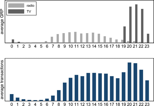
Notes. This figure shows average GRPs and sales for different times of the day. To produce this figure, we first aggregate sales at the hourly level and then, average over days and draws. We exclude the respective day of the draw because tickets can only be bought until 6 p.m. on that day, and advertising and sales are higher just before this deadline. See Figure A.3 in the Online Appendix for the pattern on the day of the draw.
We distinguish between radio and TV advertisements. TV advertisements are concentrated during evening and night hours, whereas radio advertisements are more likely to be aired in the morning and in the afternoon. This clear separation is because of the fact that, in the Netherlands, TV advertisements related to gambling must not be aired during the day, and they are allowed only as of 7 p.m.16
Figure 2 shows that GRPs are positively correlated with sales. During the hours in which sales are high, GRPs are also high. However, this does not necessarily mean that advertising has positive effects because GRPs have not been assigned randomly. For instance, it could be that consumers have more time in the evening and are, therefore, more likely to buy a lottery ticket anyway.17
Figure 3 shows GRPs and sales at the minute level for one regular draw.18 We see that the firm starts advertising on the 17th day after the last regular draw, whereas sales only increase in the last days before the draw. To explore this further, Figure A.2 in the Online Appendix shows cumulative GRPs by draw. The figure shows that the main difference across regular draws is the time at which the advertising campaign starts (where the lines start increasing) and not the advertising intensity after that (the slope of the lines). The figure also shows that the advertising intensity on the last days before the draw is higher for special draws.
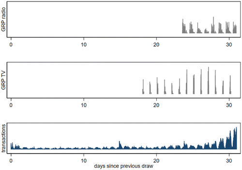
Notes. This figure shows radio and TV GRPs and sales at the minute level for the regular draw on April 10, 2014. Tickets for the next draw can be bought from 6 p.m. on the day of the previous draw, which is depicted as zero days since the previous draw.
Finally, Figure 4 zooms in further and shows the pattern for one of the days in Figure 3. Related to our identification strategy described below, it is interesting to notice that the raw data presented in Figure 4 already show some evidence of short-run sales responses to advertising. For example, there are some spikes of GRPs just before 20:50 hours, followed by spikes of sales several minutes later. In Section 6, we investigate this more systematically.
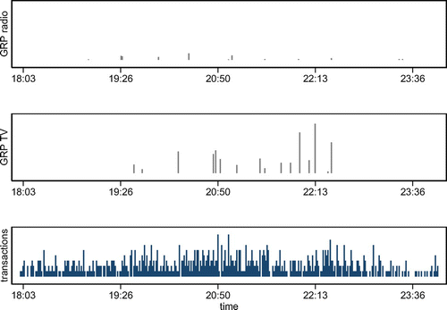
Note. This figure shows radio and TV GRPs and sales at the minute level for a short time window on April 3, 2014.
5. Advertising as a Reminder
In this section, we lay out our framework. We use it to provide a precise definition of the reminder effect of advertising. Our framework also allows for other effects of advertising. We derive a reduced-form equation and show how one can use high-frequency data to estimate the reminder effect of advertising.
5.1. Framework
There are M consumers in the market. Time t is discrete and measured in minutes. Consumers are well informed about the existence of the product. In each period, consumers may think about buying a ticket. If they think about buying, they either buy or not.
First, consider the baseline situation without advertising. Baseline quantities at time t are indexed by 0t. Denote the probability of thinking about buying by , the probability of buying given that a consumer is thinking about buying by , and the probability of buying by . From this, it follows that the baseline probability of buying is given by and that baseline sales are given by .19
Relative to this baseline, consider a counterfactual world in which an advertisement reached a consumer at t0. For , this advertisement has two effects, one on the probability of thinking about buying and another on the probability of buying given thinking.
The first effect of the advertisement is that it changes the probability of thinking about buying from to , where denotes time relative to t0. We call the reminder effect of advertising. Note that this reminder effect depends on the time since the advertisement reached the consumer. We think of it as short lived in the sense that we expect to go to zero within a few hours. Formally, we assume that there is a so that for all . The underlying way to think about consumers is that they are exposed to limits of information processing power and attention and may, therefore, forget to make an intended purchase. An advertisement reminds them of this in the sense that it draws attention to their intended purchase, but this effect on attention fades away quickly.
Figure 5 illustrates. The plot on top shows how the probability of thinking about buying, , is influenced by the advertisement. Until t0, the time at which the advertisement is aired, it is equal to the baseline probability . Then, it increases until t1 and decreases again until t2, when the probability of thinking about buying is back to the baseline level . The difference between and is equal to , and the figure shows that for and .
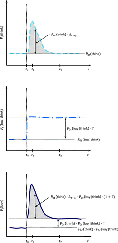
The second effect of the advertisement is that it changes the probability of buying given that the consumer is thinking about buying to . In our context, this is the effect of information about the jackpot size. More generally, this could be any effect that advertising has on the attitude a consumer has toward buying the product given that she thinks about buying. This could be either because the advertisement changes preferences or acts as a complement to consumption, or because it contains information. In our context, advertisements often name the jackpot size. If it is higher than consumers expect, then Γ could be positive. The defining characteristic of this effect is that it is long lived. In line with this, note that Γ is not indexed by τ. In Figure 5, the plot in the middle shows a situation in which . Until t0, is equal to the baseline, , and then, it changes to and remains at .
The overall effect of advertising is a change in the probability of buying from to . The bottom plot of Figure 5 shows that before t0, . After t0, first increases until t1 to and then, starts to decrease to the new level , at which it remains from t2 onward.20
5.2. Reduced-Form Equation
Above, we have considered the case in which there was one advertisement. This was useful to convey the main idea. In our empirical analysis, we take into account that there are multiple advertisements and allow for differences in the effects between radio and TV advertisements.
In Online Appendix B, we derive a reduced-form equation that is linear in lags of advertising. For this, we first express sales at time t, salest, as a function of lags of GRPs for radio and TV advertising, and , respectively. Then, we perform a Taylor series expansion in those lags about zero. This gives
To take this to the data, we form one-hour time blocks and decompose αt into a component that is specific to the time block t lies in, , and a second residual component that also contains the approximation error. This gives our reduced-form estimation equation:
5.3. Identification
Identification proceeds in two steps. First, we show identification of the coefficients and . Then, we show how one can identify and Γ from them.
5.3.1. Identification of and .
For identification of the coefficients and on the lag terms in (2), we make the following assumption.
(No Endogeneity at the Minute Level). The residual component in period t is independent of and in period s for all combinations of s and t.
This assumption means that the number of GRPs for both types of advertisements and in all periods s, including t, is not systematically related to . Importantly, Assumption 1 still allows for a relationship between , and . For instance, it allows for more advertising on days closer to the day of the draw, more advertising during certain hours of the day, and more advertising for draws with a higher jackpot. This is important because one would expect baseline sales and advertising levels to be positively correlated.
For two reasons, we expect Assumption 1 to hold in our context. First, advertising buying takes place several weeks in advance. The company chose not to determine exact times at which the advertisements were aired because this would have been more expensive. It instead indicated in broad terms when and how much advertising should be aired. We do not know specifics about this, but we have been assured that the time window was at least several hours long.
Second, the company bought a certain quantity of consumers who were reached (measured in GRPs) and not a certain number of spots that were aired. For a given time in the future, it is uncertain how many viewers will be reached, as viewership demand depends on many factors other than the TV schedule: for instance, the weather. This means that the target quantity bought by the firm is allocated to multiple spots until the amount of advertising that was actually bought has been provided (see also Dubé et al. 2005). For each of these spots, even if the time was known in advance (which it is not), the number of GRPs would not be known at the time advertising is bought.
Under Assumption 1, we can estimate the coefficients on the lag terms, and , by regressing the log of sales on lags of GRPs for radio advertising and lags of GRPs for TV advertising while controlling for time block fixed effects. To see why minute-level data are useful to estimate and , we can start from (2) and take the first difference in t. For any minute but the first of a block, this eliminates the time block fixed effect . Consider a situation where there is only a radio advertisement in t. Then, will be informative about , will be informative about , and so on. Once we know and all , we can recover all . This means that we can also estimate .21
5.3.2. Identification of , , and .
To identify , , and , we restate the restrictions we impose on the advertising effects in the following assumption.
(Advertising Effects). (i) and for , (ii) both and are constant for , and (iii) .
Part (i) says that the reminder effect for both types of advertising lasts for at most periods, part (ii) says that the effect of both types of advertising on is constant for at least periods, and part (iii) says that we have included enough lag terms in (2). In Figure 5, , which means that the model would have to include at least lag terms.
Under Assumption 2, it follows from (1) that and for (recall that ; this means that this argument applies for all ). Hence, and are identified.22 Once we know and , we can recover the parameters and , as it follows from (1) that
6. Reduced-Form Analysis
6.1. Direct Evidence for Big Advertisements
In our data, there are a number of relatively small advertisements. This means that there is often only a short amount of time between advertisements. For that reason, providing direct evidence on the effect of advertisements is challenging, as advertising effects may overlay each other. Our first approach to overcome this challenge is to select advertisements with at least 10 GRPs and only to keep the ones of these advertisements for which we do not see another big advertisement in the hour before and after. This leaves us with 44 advertisements. All of them are TV advertisements. Figure A.6 in the Online Appendix shows which advertisements were used.
We form time blocks that are 121 minutes long and cover the two hours around the time the advertisement was aired. We drop the rest of the data. Then, we nonparametrically regress sales on the time to and since the advertisement was aired.23 We rescale the estimates to obtain a figure that corresponds to in (2).24
Figure 6 shows the resulting plot of the percentage difference in sales (relative to average sales in the hour before the advertisement was aired) against the time to and since the advertisement was aired. Notice that sales are flat in the 60 minutes before the advertisement was aired, in line with the idea that these constitute a baseline that can be extrapolated. Against that baseline, we find that the effect of a big advertisement is an increase in sales that lasts for about 30 minutes. The effect is fairly immediate and dies out relatively quickly. It is a bit higher than 5% after a few minutes and overall leads to an increase of sales by 1% in the hour after it is aired.25 Thereafter, sales return to the baseline before the advertisement, suggesting that, at least on average across all big advertisements (and therefore, across draws), the information contained in advertisements does not have a longer-lasting effect (i.e., that on average is zero). It then follows from (3) that , which means that Figure 6 shows for .
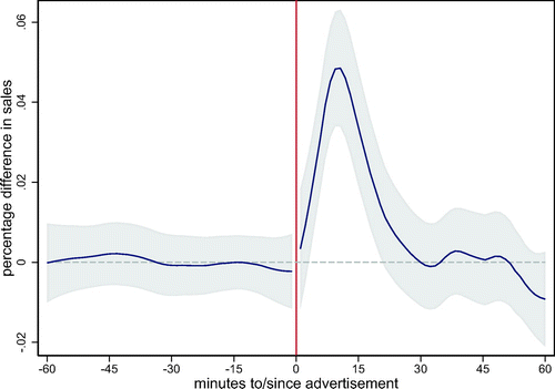
Notes. This figure shows the effect of one GRP of advertising on sales. The shaded area depicts pointwise 95% confidence intervals. See the text for additional details.
6.2. Evidence from a Distributed Lag Model
To provide more systematic evidence without selecting advertisements, we next estimate a distributed lag model. For this, we start from (2). We assume that the length of a time block is an hour. Moreover, we impose that and are piecewise constant in τ in blocks of five minutes. The reason is that we specify in our baseline specification and would otherwise have to estimate two times 240 coefficients on two times 240 lag terms. This is possible in principle, but it is too flexible in practice and produces noisy estimates. Using blocks of five minutes reduces this to lag terms, which turns out to be manageable in our situation.
The model we estimate is
The first lag term is the sum of the GRPs for radio advertising in t and the previous four minutes and has coefficient . The variable is defined accordingly for TV advertising. The second lag is the sum of the GRPs of radio advertising between nine and five minutes in the past and has coefficient , and so on. Finally, we add one to sales before taking the log, as sales are sometimes zero in our data.26 We then use the fixed effects estimator to estimate the two times 48 coefficients and on the two times 48 lag terms, controlling hour-of-year fixed effects . As for inference, we cluster standard errors at the daily level. This means that we allow for a correlation of within a day.
Figure 7 shows the results. We find that the effect of radio advertising increases until about two hours after the advertisement was aired and then, decreases. In contrast, the effect of TV advertising increases until 10–14 minutes after the advertisement was aired and then decreases. The reason for this difference in shape between the two effects could be that consumers are more likely to be at home when they watch TV and can, therefore, react faster once they are reminded.
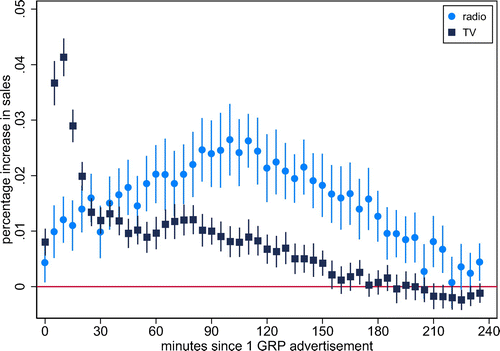
Notes. This figure shows estimates from a distributed lag model that was estimated at the minute level. The figure plots coefficient estimates on the two times 48 lags of GRPs of radio and TV advertising, respectively. The lags are each for five-minute intervals. The dependent variable is the log of one plus sales. We control for hour-of-year fixed effects. The bars indicate 95% confidence intervals, which are based on standard errors that are clustered at the daily level.
We also calculate implied effects on sales for each of the four hours after the advertisement was aired. Recall that, for instance, for radio advertising, we have estimated 12 coefficients per hour. For the first hour, the average effect is27
The average effects for the other three hours and the average effects for TV advertising are calculated accordingly. Table 1 shows the results. The effect of radio advertising is a statistically significant increase in sales by about 1.3% of the baseline sales in the first hour. In the second hour, it is 2.3%; in the third hour, it is 1.9%, and in the fourth hour, it is 0.7%. The total effect is the sum of these four effects. We find that one GRP of radio advertising increases sales on average by 6.2% of the sales of one hour (on average, 1.55% in the first four hours). For TV advertising, the effects in the first three hours are 1.8%, 1.0%, and 0.4%, respectively. The effect for the fourth hour is close to zero and not statistically significant. The total effect is an increase in sales of 3.1% of the sales of one hour (on average, 0.78% in the first four hours). The remaining columns of the table are discussed in Section 6.3.
|

Table 1. Total Effects of Advertising by Type of Advertising and Jackpot Size
| Type and time interval | (1) | (2) | (3) | (4) |
|---|---|---|---|---|
| All draws | Low jackpot | High jackpot | Difference (3) − (2) | |
| Radio | ||||
| First hour | 0.0134 | 0.0173 | 0.0148 | −0.0025 |
| (0.0016) | (0.0031) | (0.0030) | (0.0043) | |
| Second hour | 0.0232 | 0.0258 | 0.0226 | −0.0031 |
| (0.0026) | (0.0034) | (0.0037) | (0.0050) | |
| Third hour | 0.0187 | 0.0193 | 0.0241 | 0.0048 |
| (0.0023) | (0.0032) | (0.0033) | (0.0046) | |
| Fourth hour | 0.0065 | 0.0094 | 0.0101 | 0.0008 |
| (0.0016) | (0.0029) | (0.0022) | (0.0037) | |
| Sum | 0.0619 | 0.0717 | 0.0716 | −0.0001 |
| (0.0065) | (0.0102) | (0.0081) | (0.0130) | |
| TV | ||||
| First hour | 0.0180 | 0.0137 | 0.0217 | 0.0080 |
| (0.0010) | (0.0019) | (0.0021) | (0.0028) | |
| Second hour | 0.0100 | 0.0094 | 0.0115 | 0.0021 |
| (0.0011) | (0.0018) | (0.0023) | (0.0021) | |
| Third hour | 0.0039 | 0.0056 | 0.0072 | 0.0016 |
| (0.0009) | (0.0020) | (0.0024) | (0.0031) | |
| Fourth hour | −0.0008 | 0.0004 | −0.0007 | −0.0010 |
| (0.0007) | (0.0018) | (0.0017) | (0.0024) | |
| Sum | 0.0312 | 0.0290 | 0.0398 | 0.0107 |
| (0.0026) | (0.0056) | (0.0061) | (0.0083) |
Notes. This table shows implied percentage increases in sales for radio and TV advertising. We report the effect for each of the first four hours after an advertisement was aired and the sum of these average effects. The estimates of average effects for each hour and sums of average effects in column (1) are based on equation (4). In columns (2) and (3), we report averages and sums of averages for draws with low and high jackpots, respectively. Column (4) reports the difference between column (3) and column (2). Estimates related to columns (2)–(4) were obtained jointly using a fully interacted model that was estimated using data for the last seven days before the draw. The table also shows standard errors in parentheses. These were calculated using the delta method and account for correlations of error terms within days.
6.3. Does the Effect of Advertising Depend on the Jackpot Size?
So far, we have estimated reduced-form advertising effects, and . Next, we investigate whether the effects depend on the jackpot size. This could be the case, as advertisements also contained information about the jackpot size.
Recall that, according to (1) in Section 5, we have that, for instance for radio advertising, . In words, the reduced-form advertising effect is a function of the reminder effect , which does depend on the time since the advertisement was aired, and the effect of the information contained in the advertisement on . Information that lets consumers positively update their priors on the jackpot size may increase the probability of buying given that the consumer thinks about buying. Information that lets consumers negatively update their priors may lead to a decrease in that probability. Based on this, we now test the null hypothesis that and , respectively, do not depend on the jackpot size. We do so by testing the null hypothesis that and , respectively, do not depend on the jackpot size for all τ.
For this, we create an indicator for a jackpot that is above the median jackpot we observe across draws. Then, we interact this indicator with the variables and in (4). We estimate the model using data for the last seven days before the draw. The reason for doing so is that the total number of GRPs depends on the jackpot size, as shown in Figure A.2 in the Online Appendix. Figure A.2 in the Online Appendix also shows that this is mainly because advertising for high-jackpot draws starts earlier. We control for this by using only data on the last days before the draw, when there are about equal amounts of advertising for each draw.
Figure 8 shows estimates of the advertising effect separately for TV and radio advertising and by jackpot size. For radio advertising, the estimated effects are slightly lower for above-median jackpots, but the pointwise confidence intervals for both curves overlap all of the time. For TV advertising, the estimated effects are slightly higher for above-median jackpots, but again, the pointwise confidence intervals for both curves overlap most of the time. To test this formally, recall that we estimate 48 s and 48 s for high and low jackpots, respectively. Denote the 48 parameters for radio advertising and for draws with a jackpot below the median by and the 48 parameters for draws with a jackpot above the median by . We test the joint hypothesis that for all . We do the same for TV advertising. For both types of advertising, the joint hypothesis is rejected at conventional levels of significance. For radio advertising, the F statistic is 2.18, and the p-value is zero. For TV advertising, the F statistic is 3.82, and the p-value is also zero. This establishes that, in a statistical sense, both for radio and TV advertising the shapes of advertising effects are different between high and low jackpots.
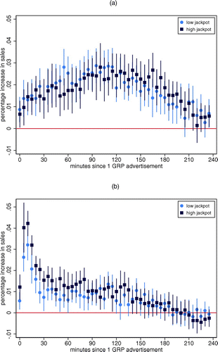
Notes. (a) Radio. (b) TV. This figure shows estimates from a distributed lag model that was estimated at the minute level. We estimate the effects by type of advertising. The first subfigure is for radio advertising. The second subfigure is for TV advertising. Estimates were obtained jointly using a fully interacted model that was estimated using data for the last seven days before the draw.
To assess economic significance, we have calculated implied average percentage advertising effects for each of the four hours after the advertisement was aired, separately for above- and below-median jackpots. Table 1 reports the results in columns (2) and (3). Column (4) reports the difference between the two. We can see that differences between the estimated average effects at the hourly level for high jackpots and the average effects at the hourly level for low jackpots are smaller for radio advertising as compared with TV advertising. The only statistically significant difference is for TV advertising in the first hour. We estimate the effect to be 58% (0.80 percentage points) higher for high jackpots.
Turning to total effects, the difference in the sum of the effects in the first four hours is very close to zero for radio advertising. For TV advertising, however, it is sizable. The total effect is statistically not significantly different between high and low jackpots but is estimated to be 37% (1.1 percentage points) higher. Overall, this suggests that next to the reminder effect, there is an effect of advertising on the inclination of consumers to buy given that they are thinking about buying, which originates in the information contained in the advertisements. However, it seems to be hard to estimate it precisely.
6.4. The Dependence of Advertising Effects on the Time Until the Draw
Reminder advertising can help consumers remember to buy a product. However, as pointed out and documented by Lambrecht et al. (2022), this does not necessarily mean that total sales increase. If consumers bought the product anyway at a later point in time, then advertising would only lead to purchase acceleration but not to market expansion.
Our empirical setup offers the opportunity to study whether advertising also leads to market expansion by making use of the fixed ending time up to which lottery tickets for a particular draw can be bought. The idea is that if advertising has an effect until shortly before the draw, then this must be because of market expansion, as there is no later point in time at which a ticket can be bought for that draw.
To study whether this is the case, we estimate a version of our model that allows for a dependence of advertising effects on the time until the draw. The reason why we need to allow for such a dependence is that baseline sales are naturally higher shortly before the draw (see Figure 1), and our estimation equation, (4), implies that short-term advertising effects are proportional to baseline sales. In our framework, proportionality arises naturally because advertising that acts as a reminder affects the probability of thinking about buying, which multiplies the probability of buying given that the consumer thinks about buying. However, we do not want to impose that here.
The more general specification includes additional interaction terms between the days until the draw and the GRP lags, so that the model is flexible enough to also capture a situation where advertising has no effect shortly before the draw. Our estimation equation is
Here, denotes the hour since the advertisement was aired, DTD(t) denotes the days to the draw, d(t) denotes the draw, and HOD(t) the hour of day. The model differs from the baseline model, (4), in two ways. First, we use draw fixed effects , days-to-draw fixed effects , and hour-of-day fixed effects . This replaces the more flexible hour-of-year fixed effects. We use this slightly more restrictive specification because it makes it easier to predict baseline sales in order to produce a figure where we plot absolute advertising effects against the days until the draw.28
The second and main way in which the model differs is that advertising effects are allowed to depend on the number of days until the draw. As in (4), we have two times 48 five-minute lag terms with coefficients and . Now, in addition, we have four times 20 interaction terms between the lag length at the hourly level, , and the last 20 days until the draw. This is best illustrated with an example. Suppose we are interested in the effect of a radio advertisement on sales 90–94 minutes later, when there are six days until the draw. indexes time blocks with length five minutes, relative to the time of the advertisement (the first block takes minutes 0–4, the second block takes minutes 5–9, and so on). This means that 90–94 minutes later corresponds to . This is in the second hour after the advertisement was aired, so . We are interested in the effect when there are six days until the draw, so DTD(t) = 6. Therefore, in this example, the effect on is given by .
Note that this specification allows for a difference in the effects of advertising between radio and TV advertisements. However, it imposes that the dependence of the effects on the time until the draw is the same for both types of advertising.
Figure 9 plots the predicted absolute advertising effects for one GRP of advertising in the first hour after an advertisement was aired relative to the absolute effect on the day of the draw. These are given by .29 The figure also shows respective 95% confidence intervals.30 Toward the time of the draw, the effects increase, which suggests that advertising leads not only to purchase acceleration but also, to market expansion.
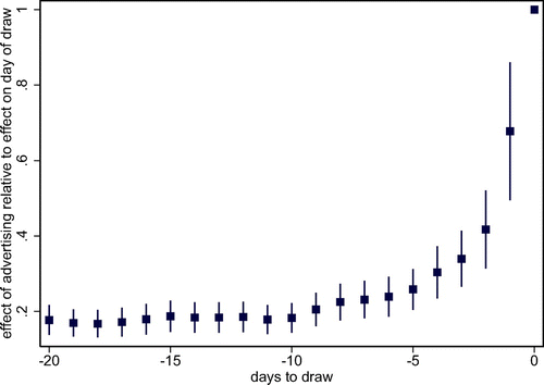
Notes. This figure shows the absolute effect of advertising on the 20 days before the draw relative to the absolute effect on the day of the draw. See the text for details.
One can also see this analysis as a robustness check related to the proportionality built into our framework and our baseline specification (4). Figure A.12 in the Online Appendix shows that the percentage effect of advertising, , does not depend statistically significantly on the time until the draw. This means that advertising effects are approximately proportional to baseline sales.
6.5. Robustness
In this section, we report results from two robustness checks and provide a brief overview over additional robustness checks that we report on in the Online Appendix. We generally do not distinguish between radio and TV advertising in our robustness checks.31
Sales and advertising levels are higher on certain days and at certain times of the day. Therefore, it is important to control for time effects. Figure 10 shows how the estimated advertising effect depends on the way we control for time effects. Corresponding coefficient estimates for the first 12 lags are reported in Table A.2 in the Online Appendix. We expect that advertising effects are overestimated if we do not control for time effects at all. The figure confirms that. At the same time, we see that advertising effects are relatively similar when we control for either hour-of-year fixed effects or time dummies (as we do in Figure 9) and even when we only control for days until the draw and a night dummy that takes on the value of one in the hours between midnight and 7 a.m. This last specification is inspired by Figure 2, showing that there is a big difference in both sales and advertising levels between day and night. The results suggest that controlling for the time of the day in terms of day and night is sufficient to alleviate endogeneity concerns. We will make use of this when we estimate the structural model.
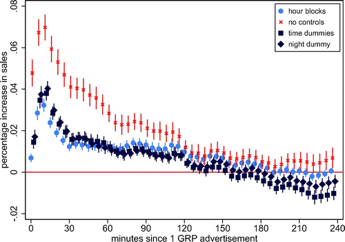
Notes. This figure shows estimates from a distributed lag model that was estimated at the minute level. There are 48 lags that are each for five-minute intervals, so four hours in total. The four curves are for four different sets of controls: hour-of-year fixed effects, no controls, time dummies, and a night dummy. The dependent variable is the log of one plus sales. The bars indicate 95% confidence intervals, which are based on standard errors that are clustered at the daily level. Table A.2 in the Online Appendix shows the coefficients for the first 12 lags.
Our second robustness check is to report results for a set of placebo advertisements. We generate the placebo advertisements by first generating an indicator for there being an advertisement in a given minute. We take the likelihood that this is the case from the data, pooling over time. Then, we draw the number of GRPs from a lognormal distribution with the same mean and variance as the distribution of GRPs conditional on there being an advertisement in the data. This means that we will have twice as many advertisements in the new data than before. Starting from this, we estimate a model that simultaneously estimates the effect of the actual advertisements and the placebo advertisements. For this, we use the same specification as in Figure A.7 in the Online Appendix but add 48 additional lag terms for the placebo advertisements. Figure 11 shows the results. The effect of the placebo advertisements is estimated to be very close to zero, with very tight confidence intervals, whereas the estimated effect of the actual advertisements is very close to the one we have estimated.
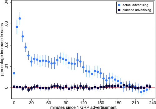
Notes. This figure shows estimates from a distributed lag model that was estimated at the minute level. We jointly estimate the effects of the actual advertisements that were aired and a set of placebo advertisements that were placed at random times. See the text for details.
Taken together, these two robustness checks suggest that advertising effects are well identified. In the Online Appendix, we carry out a number of additional robustness checks. We show that aggregating data to the hourly level leads to similar estimates of advertising effects (Table A.4 in the Online Appendix); that estimating the model with shorter time blocks leads to similar results (Figure A.8 in the Online Appendix); that the estimated effect per GRP does not strongly depend on whether many or not so many consumers have been reached (Figure A.9 in the Online Appendix); that the effects for big TV advertisements are similar to the effects of all TV advertisements (Figure A.10 in the Online Appendix); that coefficients on lead terms are close to zero (Figure A.11 in the Online Appendix), which can be seen as an additional placebo check; and that percentage advertising effects do not depend on the time until the draw (Figure A.12 in the Online Appendix).
7. A Model of Lottery Ticket Demand
Our reduced-form analysis is well suited to estimate the short-run effects of advertising. However, we cannot use it to conduct counterfactual experiments in which we change the advertising schedule for a longer time period. The reason is that our reduced-form analysis does not capture that consumers who are motivated to buy a ticket will be less inclined to buy another one in the future, even if they are reminded again.
In this section, we estimate a simple structural model to gain more insight into the medium-run effects of advertising. The model is static, and the length of one period is one hour. Consumers stay in the market until they buy a ticket or the draw takes place. Therefore, the mechanism through which medium-run advertising effects arise is that consumers buy and leave the market instead of staying in the market and possibly buying a ticket.
The probability of thinking about buying a ticket is given by a simple logit specification:
Here, advertising enters through an advertising goodwill stock, , the evolution of which we simulate for a hypothetical set of consumers. It depreciates from period to period with rate λ. Our data are informative about how many consumers are reached by an advertisement. This information is used to select randomly the appropriate number of simulated consumers whose goodwill stock is additionally increased by one unit.
The probability of buying (for the consumers who are still in the market) given that the consumer thinks about buying is specified as
Here, we normalize the price coefficient to one. The term captures that the value to buying a ticket depends on the time until the draw. In Figure 9, we document that advertising effects are bigger when there is less time until the draw. This can be captured by our specification, with a value of δ smaller than one. We treat both δ and ψ as parameters and divide average utility by the scaling factor σ.
We estimate the model using the method of simulated moments.32 With our parameter estimates in hand, we turn to the question what the effect of alternative dynamic advertising schedules would have been, including the case of no advertising at all. We do not have access to data on the profitability of an additional sold ticket nor on the cost of one GRP. However, it is not unreasonable in our context to assume as an approximation that the price of one GRP does not vary over time, especially because the firm decided not to buy advertising at prespecified times and regular draws are on the 10th day of the month, independent of the weekday. In that sense, it is meaningful to ask the question of whether it is possible to sell more tickets when one allocates the same number of GRPs in a different way.
We consider four alternative strategies and compare the total number of tickets sold with the simulated one for the original GRP schedule in the data. The first alternative strategy is to remove all advertising. Comparing sales under this strategy with baseline sales will allow us to estimate what the overall effect of advertising was. In the second alternative strategy, we allocate all advertising to the last four days before the draw and distribute it equally over all hours on those four days. This allows us to estimate the effect of shifting advertising to times at which consumers are more likely to buy given that the consumer thinks about buying. This counterfactual strategy, however, is completely artificial and does not take scheduling constraints into account. To gain some insight into the effect of more realistic changes, the last two counterfactual strategies take the schedule as it is in the third week and move it to the fourth week (i.e., adding it to the one in the fourth week) and vice versa, respectively.
Table 2 shows the results. Not advertising at all leads to 83.3% of the original sales. Generally, allocating advertising to later points in time increases sales. The most drastic measure we considered was to move all advertising to the last four days before the draw. This leads to an increase in sales of 13.7%. The more realistic experiment of moving advertising from the third to the fourth week still leads to an increase in sales of 9.2%. The converse, namely to move advertising from the fourth week to the third, lead to a decrease in sales by 13.8%.
|
Table 2. Effect of Various Advertising Strategies
| Strategy | Sales, % |
|---|---|
| Data (reference point) | 100.0 |
| No advertising at all | 83.3 |
| Spreading advertisements equally in the last 4 days before the draw | 113.7 |
| Shift advertising from third week to fourth week | 109.2 |
| Shift advertising from fourth week to third week | 86.2 |
Notes. This table shows the effect of using alternative dynamic advertising strategies for the February draw. See the text for a description of these strategies. Simulations are based on the parameter estimates reported in Table A.5 in the Online Appendix.
Figure 12 shows the underlying dynamics. We plot the difference between the cumulative sales for a given strategy and the baseline strategy. For example, consider the strategy of shifting all the GRPs from the fourth week to the third week. As expected, sales in the third week increase faster than sales for the baseline strategy (hence, the difference in cumulative sales is positive). Thereafter, they fall behind (hence, the difference is negative). Overall, fewer tickets are sold, which is reflected in the lower end point.
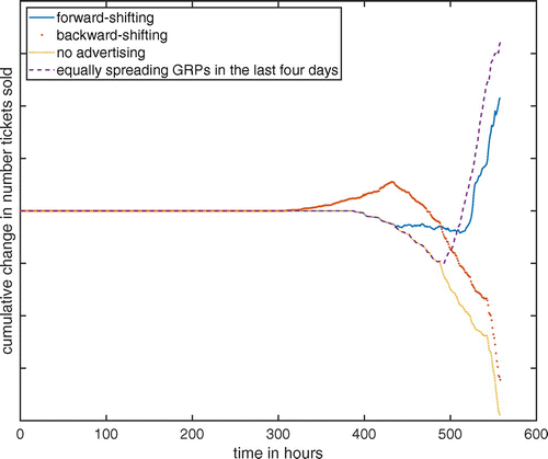
Notes. This figure shows the difference between the cumulative number of tickets sold at each point in time for a counterfactual advertising strategy and the cumulative number of tickets sold given the actual advertising schedule for the February draw. It is based on the parameter estimates reported in Table A.5 in the Online Appendix.
8. Concluding Remarks
In this paper, we provide empirical support for the view that advertising can act as a reminder when consumers suffer from limited attention. We focus on one particular context—online sales of lottery tickets in the Netherlands—that is particularly well suited for this purpose. We propose a new framework in which advertising can act as a reminder, and we develop an empirical approach that allows us to isolate reminder effects from other effects of advertising, in particular those influencing consumer choice because advertisements contain information about the jackpot size. We then use high-frequency data to credibly identify and estimate the short-run reminder effects of advertising. We also propose a simple structural model with an attention stage and estimate its parameters to gain insights into medium-run effects.
We find the short-term effects of advertising to be strong. Reaching 1% of the population by a radio advertisement leads to an increase in online sales of 1.55% in the first four hours after the advertisement is aired. The effect is an increase of 0.78% for a TV advertisement. This can be attributed to advertising acting as a reminder. We show that reminder advertising can lead to market expansion and that shifting reminder advertising to times at which consumers want to be reminded can have substantial effects on sales. Our counterfactual predictions suggest that total online sales would be 16.7% lower without the reminder effect of advertising and that shifting advertising to the week of the draw can lead to an increase in total online sales of 9.2%.
There are four managerial implications for firms that consider using advertising as a reminder. First, it is important to reach consumers at a time and in a situation in which they are ready to make a purchase. In our context, this is the case shortly before the draw. In other contexts, such as for insurance that is bought for a calendar year, this could be shortly before the start of the new year. Second, advertisements that are meant to remind consumers could be designed specifically for that purpose and could be shorter, in particular if many consumers are already aware of the product and are well informed about it. Third, for reminder advertising to be successful, it is important that consumers make a purchase before attention fades away. Our results suggest that this is the case within four hours. Therefore, it is important to make it as easy for consumers as possible to buy the product online as soon as they want to do so. Fourth, reminder advertising could be used in combination with other marketing instruments. For example, advertisements could remind consumers of the end date of a special sale or the expiration date of a coupon.
Reminder advertising helps consumers act on their preferences. By proposing a new empirical framework and providing evidence for this pathway, we hope to stimulate more work on the topic. This seems important to us, as many fundamental results in economics and marketing hinge on the presumption that consumers do indeed act on their preferences.
The authors thank Blue Mango Interactive and the Dutch State Lottery for providing the data; the views expressed in this paper, however, do not necessarily reflect those of Bluemango or the Dutch State Lottery. The authors thank Menno Zevenbergen and Pieter van Geel for stimulating discussions and useful comments; without them, this project would not have been possible. They also thank Senior Editor Puneet Manchanda, the associate editor Günter Hitsch, two anonymous referees, Jean-Pierre Dubé, Ulrich Doraszelski, Eric French, Ulrich Kaiser, Carl Mela, Peter Newberry, Martin Peitz, Pasquale Schiraldi, Stephan Seiler, Andrey Simonov, Rik Pieters, Frank Verboven, Ken Wilbur, Joachim Winter, participants of a seminar in Oxford, participants at eBay in San José, and participants of the 2015 Media Economics Workshop in Stellenbosch, the 2016 meeting of the Industrial Organization group of the Verein für Socialpolitik, the 2016 Digital Marketing Conference at Stanford, the 2017 Center for Economic and Policy Research Conference on Applied Industrial Organization, the 2018 European Economic Association/Econometric Society European Meeting in Cologne, and the 2019 Choice Symposium in Chesapeake Bay for their for comments and suggestions.
1 About 90% of the sales still take place offline. In Section 3, we discuss implications of this for the interpretation of our results.
2 In our analysis, we focus on short-run effects of advertising. The advertisements could also have longer-run effects that are not related to the reminder effect of advertising. Our empirical approach allows for this, but we are not able to separately identify those longer-run effects with our identification strategy. See footnote 22.
3 We thank Martin Peitz for this suggestion.
4 Summarizing this literature is beyond the scope of this paper. See Bagwell (2007) for an excellent survey on the economics of advertising.
5 There is also a large broader literature on inattention. See Gabaix (2019) for an excellent survey.
6 In a previous version of this paper, we also estimated a dynamic model with an attention stage. The results of counterfactual experiments were very similar.
7 In 2014, the Dutch State Lottery had a turnover of 738 million euros, with 579 million euros related to its lottery; De Lotto had a turnover of 322 million euros, with 144 million euros related to its lottery (https://over.nederlandseloterij.nl/over-ons/publicaties, accessed February 2022). The turnover of Nationale Goede Doelen Loterijen was 847 million euros in total, with 624 million euros related to its charity zip code lottery (https://view.publitas.com/nationale-postcode-loterij-nv/npl-jaarverslag-2014/page/58-59, accessed February 2022).
8 For an example, see https://www.loten.nl/staatsloterij/ (accessed February 2022).
9 The effect on online sales is likely a lower bound on the effect on total sales. The first effect on offline sales is likely positive. The second effect only leads to online sales instead of offline sales; total sales are not affected by it.
10 These data have been collected using Google Analytics. In particular, visits to the “exit page” confirming payment have been recorded. This means that we do not observe what type of ticket a consumer has bought. Advertising also affects offline sales, and therefore, we would ideally also like to observe the number of lottery tickets sold offline. However, offline transactions are not observed in the data set. At the same time, it generally takes longer until an offline sale takes place after an individual has listened to a radio advertisement or seen a TV advertisement. At the minimum, this will be the time it takes between listening to a radio commercial in the car and buying a ticket in a shop. Therefore, it will be much more challenging to measure advertising effects in offline data—a challenge we try to overcome with our high-frequency online sales data. For the interpretation of our results, we focus on online sales.
11 Our data do not contain information on the number of times consumers are reached by the advertisements. This means that we will estimate the average effect of advertising, where the average is taken over the number of times a consumer is reached. We conduct a related robustness check for our structural model in Online Appendix D.8.3.
12 Patterns for the other draws are similar. See Figure A.1 in the Online Appendix for the remaining draws.
13 We do not expect this to have big effects, because most tickets are sold in the week before the draw. However, we do take this into account in our analysis.
14 See Table A.1 in the Online Appendix for details.
15 See Figure A.3 in the Online Appendix for the pattern on the day of the draw.
16 We have tried to exploit this regression discontinuity design to produce estimates of advertising effects. However, it turns out to be difficult to distinguish the discontinuity in the total number of GRPs from a flexible time trend. The reason is that the number of GRPs increases in a continuous manner between 7 and 9 p.m. and did not sharply jump to a high level right after 7 p.m.
17 This is a well-known challenge for the analysis of advertising effects. Our identification strategy for overcoming this challenge is described in Section 5.
18 Figure A.4 in the Online Appendix shows GRPs and sales for the special draw on April 26. Patterns are similar.
19 One can generalize this model by introducing consideration sets. A consideration set contains the products a consumer is aware of. Then, the probability of buying is the product of three probabilities: the probability of thinking about buying, the probability that the product is in the consideration set (which does not depend on whether the consumer thinks about buying), and the probability that the consumer buys given that the product is in the consideration set and that she thinks about buying. In our case, the consumer is well informed about the existence of the product, and therefore, we have that the probability that the product is in the consideration set is equal to one.
20 Part of the increase in the probability of buying between t0 and t1 could be driven by consumers going through the buying process on the website. Here, we attribute this to an increase in the probability of thinking about buying. The model could be generalized to allow for a delay between the decision to buy and the actual purchase. Then, we could model the probability of thinking about buying as jumping up at t0 and then, monotonically decreasing until t2, without a peak at t1. Importantly for our analysis, even without this generalization, we can still interpret the shaded area in the bottom plot as the reminder effect of advertising on sales, as it is caused by an increase in the probability of thinking about buying. The reason is that a delay between the decision to buy and the actual purchase does not change the size of that area. It only shifts the timing of the additional purchases (the shape of the area but not its size).
21 This is obviously not a formal proof of identification. For a more formal argument, assume that Assumption 1 holds for . Then, the fixed effects estimator will consistently estimate the parameters and under a standard rank condition.
22 After periods, this long-run effect is captured by the parameters .
23 We use separate nonparametric regressions for the times to and since the advertisement was aired, respectively. We used a local constant specification and the rule-of-thumb bandwidth.
24 Denote estimates by , average TV GRP in the sample by , and average sales in the hour before the advertisement was aired by . Figure 6 shows .
25 This is the average estimated value in the first hour.
26 Usually, and are interpreted as approximately a percentage change in sales, as they approximate the actual percentage changes and very well for small values of and . This is still the case when we use the log of one plus sales as the dependent variable. To see this, assume that baseline sales are equal to 10 and that the actual effect of one GRP of radio advertising is a 4% increase in sales to 10.4. Then, we have that . This means that our coefficient estimate would be 0.036.
27 This would be exactly the percentage change if our dependent variable was the natural logarithm of sales. However, we use the natural logarithm of one plus sales as the dependent variable. See footnote 26.
28 This is supported by our first robustness check in Section 6.5.
29 We normalize for the day of the draw, for the first draw, for the day of the draw, and for the first hour of the day. It follows from (5) that . The normalizations imply that on the day of the draw, keeping everything else equal, this is . Taking the ratio of the two and evaluating it for one GRP in the hour before t gives .
30 We have also tried to “zoom in” and show that the effect is there in the very last hours before the draw, but we only have data for 16 draws, with a limited number of advertisements in the last hours before the draw.
31 See Online Appendix C.1 for details on this simpler specification.
32 We provide additional technical details in Online Appendices D.1–D.3. Online Appendix D.4 discusses identification of the structural parameters. Technical details related to estimation are discussed in Online Appendix D.5. Online Appendix D.6 reports parameter estimates and shows that the model fits the data well. Online Appendix D.7 shows how we can use the model to calculate the elasticity of sales with respect to advertising. We find that it is 0.0414, which is in line with the ones found in some other contexts. In Online Appendix D.8, we assess the robustness to making alternative assumptions on the market size and viewership behavior.
References
- (2021) What do consumers consider before they choose? Identification from asymmetric demand responses. Quart. J. Econom. 136(3):1611–1663.Crossref, Google Scholar
- (2001) Empirically distinguishing informative and prestige effects of advertising. RAND J. Econom. 32(2):316–333.Crossref, Google Scholar
- (2003) Advertising, learning, and consumer choice in experience good markets: An empirical examination. Internat. Econom. Rev. 44(3):1007–1040.Crossref, Google Scholar
- (1995) The effects of in-store displays and feature advertising on consideration sets. Internat. J. Res. Marketing 12(1):67–80.Crossref, Google Scholar
- (2007)
The economic analysis of advertising . Armstrong M, Porter R, eds. Handbook of Industrial Organization, vol. 3 (Elsevier, Amsterdam), 1701–1844.Google Scholar - (1995) How promotions work. Marketing Sci. 14(3):G122–G132.Link, Google Scholar
- (1996) Limited choice sets, local price response, and implied measures of price competition. J. Marketing Res. 33(2):163–173.Crossref, Google Scholar
- (2016) Effective reminders. Management Sci. 63(9):2915–2932.Link, Google Scholar
- (2018) Effects of offline ad content on online brand search: Insights from Super Bowl advertising. J. Acad. Marketing Sci. 46(3):403–430.Crossref, Google Scholar
- (2019) Subsidies and time discounting in new technology adoption: Evidence from solar photovoltaic systems. Amer. Econom. Rev. 109(6):2137–2172.Crossref, Google Scholar
- (2010) Persuasion: Empirical evidence. Annual Rev. Econom. 2(1):643–669.Crossref, Google Scholar
- (2011) Choice set heterogeneity and the role of advertising: An analysis with micro and macro data. J. Marketing Res. 48(4):653–669.Crossref, Google Scholar
- (2019) Immediate responses of online brand search and price search to TV ads. J. Marketing 83(4):81–100.Crossref, Google Scholar
- (2005) An empirical model of advertising dynamics. Quant. Marketing Econom. 3(2):107–144.Crossref, Google Scholar
- (2019)
Behavioral inattention . Bernheim BD, DellaVigna S, Laibson D, eds. Handbook of Behavioral Economics: Applications and Foundations 1, vol. 2 (Elsevier, Amsterdam), 261–343.Crossref, Google Scholar - (2017) Super Bowl ads. Marketing Sci. 37(1):78–96.Link, Google Scholar
- (2021) Inattention and switching costs as sources of inertia in Medicare Part D. Amer. Econom. Rev. 111(9):2737–2781.Crossref, Google Scholar
- (2017) The impact of consumer inattention on insurer pricing in the Medicare Part D program. RAND J. Econom. 48(4):877–905.Crossref, Google Scholar
- (2017) Power to choose? An analysis of choice frictions in the residential electricity market. Amer. Econom. J. Econom. Policy 9(4):192–226.Crossref, Google Scholar
- (2007) An analysis of real world TV advertising tests: A 15-year update. J. Advertising Res. 47(3):341–353.Crossref, Google Scholar
- (1994) Do coupon expiration dates affect consumer behavior? J. Marketing Res. 31(3):423–428.Crossref, Google Scholar
- (2016) Effects of TV advertising on keyword search. Internat. J. Res. Marketing 33(3):508–523.Crossref, Google Scholar
- (2014) Television advertising and online search. Management Sci. 60(1):56–73.Link, Google Scholar
- (1972) Why three exposures may be enough. J. Adverting Res. 12(6):11–14.Google Scholar
- (2022) TV advertising and online sales: A case study of intertemporal substitution effects for online hotel bookings. Preprint, submitted July 28, https://dx.doi.org/10.2139/ssrn.3530105.Google Scholar
- (2013) Down-to-the-minute effects of super bowl advertising on online search behavior. Proc. Fourteenth ACM Conf. Electronic Commerce (ACM, New York), 639–656.Google Scholar
- (2015) Television advertising and online shopping. Marketing Sci. 34(3):311–330.Link, Google Scholar
- (1995) How TV advertising works: A meta-analysis of 389 real world split cable TV advertising experiments. J. Marketing Res. 32(2):125–139.Crossref, Google Scholar
- (2014) Stochastic choice and consideration sets. Econometrica 82(3):1153–1176.Crossref, Google Scholar
- (2008) Informing, transforming, and persuading: Disentangling the multiple effects of advertising on brand choice decisions. Marketing Sci. 27(3):334–355.Link, Google Scholar
- (2013) Demand for differentiated durable products: The case of the U.S. computer printer market. Econom. Inquiry 51(2):1277–1298.Crossref, Google Scholar
- (1991) Development and testing of a model of consideration set composition. J. Marketing Res. 28(4):429–440.Crossref, Google Scholar
- (1997) Consideration: Review of research and prospects for future insights. J. Marketing Res. 34(3):406–410.Crossref, Google Scholar
- (1987) Advertising and Promotion Management (McGraw-Hill, New York).Google Scholar
- (2015) Effect of temporal spacing between advertising exposures: Evidence from online field experiments. Quant. Marketing Econom. 13(3):203–247.Crossref, Google Scholar
- (2018) Positive spillovers and free riding in advertising of prescription pharmaceuticals: The case of antidepressants. J. Political Econom. 126(1):381–437.Crossref, Google Scholar
- (2021) TV advertising effectiveness and profitability: Generalizable results from 288 brands. Econometrica 89(4):1855–1879.Crossref, Google Scholar
- (2022) A “memory-jamming” theory of advertising. Working paper, University of Chicago, Chicago.Google Scholar
- (2008) Limited information and advertising in the U.S. personal computer industry. Econometrica 76(5):1017–1074.Crossref, Google Scholar
- (2017) Super returns to super bowl ads? Quant. Marketing Econom. 15(1):1–28.Crossref, Google Scholar
- (2011) The effect of media advertising on brand consideration and choice. Marketing Sci. 30(1):74–91.Link, Google Scholar
- (2010) Retrieving unobserved consideration sets from household panel data. J. Marketing Res. 47(1):63–74.Crossref, Google Scholar
- (2010) Assessing a new advertising effect: Measurement of the impact of television commercials on Internet search queries. J. Adverting Res. 50(2):162–168.Crossref, Google Scholar

