Leveraging Large-Scale Granular Single-Source Data for TV Advertising: An Identification Strategy
Abstract
This study introduces a novel instrumental variable (IV) for estimating the causal effects of linear television (TV) advertising using large-scale panel data that link household second-by-second show viewership and ad exposure with daily purchase behavior. We exploit an institutional feature of linear TV: Although advertisers choose which shows to target, networks quasi-randomly determine within-show ad airing times. This creates exogenous variation in focal brand ad exposure among partial show viewers, which we nonparametrically extract to construct a household-show-level IV. We establish the IV’s validity in the presence of endogeneity arising from advertisers’ show targeting decisions and households’ TV viewing behavior. Our IV offers a generalizable and flexible solution for household-level linear TV ad effect measurement using modern single-source data. Applying this method to data from a major food delivery platform, we estimate an ad response model in which both baseline purchase propensity and ad responsiveness vary with purchase history. Naïve estimates overstate ad elasticities by 55% compared with IV-corrected estimates. We also find that ad responsiveness is nonmonotonic with respect to purchase frequency and recency. These findings underscore the importance of addressing endogeneity in observational household TV ad exposure data and highlight the potential of behaviorally targeted TV advertising.
History: Olivier Toubia served as the senior editor for this article.
Supplemental Material: The online appendices and data files are available at https://doi.org/10.1287/mksc.2023.0582.
1. Introduction
Linear television (TV) remains one of the few media capable of reaching mass audiences in real time, particularly through live programming such as sports and major cultural events. This distinctive capacity has sustained tens of billions of dollars in annual advertiser spending despite the proliferation of digital channels. Yet the continued relevance of linear TV as an advertising medium depends on rigorous measurement of both its short- and long-term causal impact.
Unlike digital advertising, randomized controlled trials (RCTs) are largely infeasible in the linear TV context because of the broadcast nature of programming and the limited infrastructure for household-level randomization. Consequently, practitioners and academics primarily rely on observational data, where two sources of endogeneity complicate inference: targeting bias and activity bias (Lewis et al. 2011, Lewis and Reiley 2014, Zhang et al. 2017, Gordon et al. 2019). Targeting bias arises when advertisers buy placements in shows whose audiences differ in baseline purchase propensities. Activity bias occurs when household TV viewing patterns at specific times correlate with baseline purchase propensities.
Recent comparisons of observational estimates with RCT benchmarks in digital advertising show that these biases are difficult to eliminate. Neither extensive controls nor algorithmic flexibility adequately address the endogeneity inherent in the data-generating process (DGP) (Gordon et al. 2019, 2023). Most existing identification strategies for TV advertising instead rely on nonexperimental, exogenous variation in ad exposure at the market level (Hartmann and Klapper 2017, Stephens-Davidowitz et al. 2017, Shapiro 2018, Thomas 2020). Although informative, these approaches cannot capture heterogeneity across households within a market or dynamic variation within households over time.
Against this backdrop, we introduce a method to quantify the causal effects of linear TV advertising using household-level observational data that link ad exposures with purchases over extended periods. This approach is especially timely, as advertisers increasingly gain access to modern single-source data that merge second-by-second TV viewership from millions of households with first-party purchase histories.1
Our method offers two key advantages that facilitate practical adoption: generalizability and flexibility. It is generalizable because causal identification does not depend on advertiser- or campaign-specific exogenous shocks. It is flexible because it scales to millions of households, accommodates repeated ad exposures, and leverages longitudinal purchase data. Together, these features allow estimation of cross-sectional heterogeneity in TV ad effects and separation of short-term responses from long-term dynamics such as carryover and state dependence. By providing a more accurate and nuanced assessment of television advertising effectiveness, the method informs strategic refinement and reinforces linear TV’s continued role as a viable mass medium.
The core of our identification strategy leverages an institutional feature of U.S. linear TV: Although advertisers decide which shows to target, networks determine the precise timing of ad airings within those shows. To ensure fairness, networks generally implement an equitable rotation of advertisers’ ads across the available slots within a show—a practice often referred to as “quasi-random ordering” (Wilbur et al. 2013, Gordon et al. 2021, McGranaghan et al. 2022). This practice generates exogenous variation in focal brand ad exposure when a household watches only part of a targeted show, as exposure depends on whether the focal brand ad happens to air during the segment(s) the household viewed.
Building on this insight, we propose a household-show-level instrumental variable (IV) to identify the causal effects of linear TV ad exposures. Intuitively, when a household watches only part of a show targeted by the focal brand, the network’s quasi-random allocation of within-show ad slots across advertisers functions as a natural experiment, introducing a degree of randomness in realized focal brand ad exposure that is orthogonal to its endogenous determinants.
We isolate this network-induced exogenous shock by first constructing an expected focal brand ad exposure measure for each household during each targeted show. Conceptually, this measure captures the likelihood that a household would be exposed to the focal brand ad, given the portion of the show it watched and the network’s typical within-show ad insertion pattern. Empirically, it is derived from two inputs: (a) the household’s second-by-second viewership of the targeted show and (b) the empirical distribution of the network’s within-show ad airing times.
Our household-show–level IV is then defined as the difference between this expected exposure and the household’s realized treatment status. In this way, the IV captures variation in focal brand ad exposure arising not from household show viewing behavior or the focal brand’s show targeting decisions, but from the network’s quasi-random ordering of within-show ad placements.
To illustrate, suppose a household watched only the middle third of a targeted show. Based on the network’s typical within-show ad insertion pattern, 40% of ad slots would be expected to fall in the middle third, yielding an expected focal brand ad exposure of 0.4 for the household, given its viewing window and the network’s quasi-random allocation of ad slots across advertisers. If the focal brand ad did air in the middle third, the household’s realized treatment status would be 1, producing an IV of 0.6 (= 1 − 0.4). If it did not, the realized treatment status would be 0, producing an IV of −0.4 (= 0 − 0.4).
The validity of our decompositional approach to IV construction, that is, subtracting expected from realized treatment, rests on the expected component capturing all endogenous determinants of the latter, leaving only exogenous variation in the residual. In other words, our identification strategy hinges on estimating expected focal brand ad exposure in a way that fully accounts for all pathways through which unobserved confounders could affect realized exposure (e.g., via the focal brand’s show targeting decisions or the household’s show viewing behavior).
Two identifying assumptions are required for our proposed IV to be valid. First, we assume that networks assign within-show ad slots quasi-randomly across advertisers, irrespective of the identity of the focal brand or household. This “quasi-random ordering” assumption ensures a degree of exogenous variation in the precise timing of focal brand ad airing within a targeted show.
Second, we assume that a household’s viewership of a targeted show is independent of the timing of the focal brand ad within that show. In other words, households are assumed to watch or skip the focal brand ad in the same manner as ads from other brands, without selectively adjusting their viewing behavior based on whether the focal brand ad is shown. This “nonstrategic viewership” assumption allows us to estimate a household’s probability of within-show focal brand ad exposure directly from its observed viewership of the targeted show. In our empirical application, both identifying assumptions are supported by their respective diagnostic checks.
As we demonstrate through formal proofs in a general setting and a stylized numerical example with a known DGP, our proposed IV is valid and satisfies three key properties under the identifying assumptions: (a) zero mean, (b) positive correlation with realized treatment, and (c) no correlation with confounders. Although instrument exogeneity in real-world applications is inherently untestable, our construction of the IV from observables enables falsification checks that can be implemented empirically—an approach we validate through both the formal proofs and the numerical example.
We apply our method to a panel data set that combines second-by-second TV viewing data from LG Ad Solutions (LGADS) with first-party purchase data from a major food delivery platform, the focal brand in our study.2 Our data cover 1.4 million U.S. households over a 4.5-month period (November 15, 2020–March 28, 2021), linking linear TV ad exposures to daily household purchase behavior over time.
Our empirical application focuses on two primary goals. First, we demonstrate the use of the proposed IV to estimate the causal impact of linear TV advertising. We empirically verify that, across networks, the within-show timing distributions of focal brand ads are statistically indistinguishable from those of nonfocal brands, consistent with the quasi-random ordering practice in linear TV. We further show that our IV passes the falsification checks, exhibiting zero mean and no correlation with the expected treatment, thereby supporting its validity in our empirical setting.
Second, we leverage repeated ad exposures and purchases over time to examine how ad effects vary with households’ purchase histories. This is important because it allows advertisers to target TV ads—much like digital ads—not only by demographic characteristics such as age and gender, but also by past purchase behavior. As the availability of addressable TV ad inventory expands, targeting based on behavioral history is becoming increasingly relevant (Malthouse et al. 2018, eMarketer 2022).
To achieve the goals of our empirical application, we specify a household daily ad response model in which baseline purchase propensity and ad responsiveness vary with purchase frequency (i.e., number of past purchases) and recency (i.e., days since the last purchase). To correct for endogeneity, we incorporate the proposed IV via a control function term in the latent utility of a probit purchase model.
Two key findings emerge. First, failing to correct for endogeneity results in a 55% overstatement of TV ad effectiveness: Average same-day (30-day) ad elasticity declines from 0.072 (0.222) to 0.045 (0.143) after IV correction. Second, both baseline purchase propensity and ad responsiveness vary systematically with purchase history, consistent with state dependence. For baseline purchase propensity, we observe a “habit formation” effect, whereby a prior purchase increases the likelihood of a subsequent one, and a “recency trap” effect, whereby the likelihood of a new purchase declines as more time passes since the last purchase. For ad responsiveness, we find an inverted U-shaped relationship with purchase frequency and a U-shaped relationship with purchase recency.
Together, these findings underscore (a) the debiasing power of the proposed IV and (b) the value of targeting TV ads based on household purchase history. Whereas causal inferences from aggregate data obscure cross- and within-household variation in ad exposures and responses, estimates derived from modern single-source data yield a more accurate and nuanced understanding of TV ad effects. This, in turn, enables advertisers to better determine which consumers to target and when. Our methodological advance thus provides a powerful tool for enhancing the return on investment (ROI) of TV advertising.
2. Related Literature and Intended Contributions
Our research contributes to a growing body of work developing identification strategies to estimate the causal impact of TV advertising using observational data. Table A1 in Online Appendix A summarizes selected studies focused on causal identification in this area. Notably, most existing strategies are designed for market-level rather than household-level data. For instance, Hartmann and Klapper (2017) and Stephens-Davidowitz et al. (2017) exploit regional shocks in exposure to national Super Bowl ads to identify their effects. Shapiro (2018) leverages variation in TV ad exposures across Designated Market Areas (DMA) border areas, whereas Thomas (2020) exploits spillovers of mass media advertising into smaller local markets.
Li et al. (2024) develop an IV based on preference externalities, wherein an individual’s treatment depends on the preferences of others in the group. Sinkinson and Starc (2019) and Moshary et al. (2021) identify the causal effect of TV advertising by exploiting shocks in demand for political ads during election cycles. Joo et al. (2014), Liaukonyte et al. (2015), and Du et al. (2019) leverage the precise timing of TV ad insertions and use narrow temporal windows (e.g., one hour before and after) to identify immediate effects on aggregate consumer responses at the brand level. McGranaghan et al. (2022) apply a similar approach to individual-level data, focusing on the immediate effect of ad exposure on TV viewing behavior (i.e., tuning, presence, and attention), and treat ad exposures as exogenous under the quasi-random ordering of ads within a show.3
We advance the literature on causal identification in TV advertising by introducing a novel, generalizable IV using household-level observational data. Although prior studies have leveraged the quasi-random ordering of ads within a show (Liaukonyte et al. 2015, McGranaghan et al. 2022), our contribution lies in how this variation is exploited: We construct an instrument as the residual between a household’s realized treatment and its expected treatment conditional on the household’s second-by-second show viewership and the network’s empirical distribution of ad placements across show durations.
Our research also contributes to the literature on the effects of TV advertising on household purchase dynamics using single-source data. Table A2 in Online Appendix A highlights the features that set our work apart from earlier studies. Unlike traditional scanner panel-based single-source data, the modern single-source data employed in our study provide substantially greater scale and granularity. For example, our panel of 1.4 million households is at least two orders of magnitude larger than the single-source panels used in prior studies (e.g., 1,775 households in Ackerberg (2001, 2003)). This scale provides the statistical power necessary to implement our identification strategy and to capture dynamic ad effects such as state dependence.
Another distinctive aspect of this research is our approach to capturing how the impact of TV advertising evolves with households’ past purchases. Accounting for these dynamics is essential because, for example, the effectiveness of TV advertising may be overstated if intertemporal substitution is ignored (Lambrecht et al. 2023) or understated if accelerated habit formation is not considered. Our identification strategy and ad response model enable advertisers to assess the relative efficacy of targeting TV ads not only by broad demographic characteristics such as age and gender but also by purchase frequency and recency. This perspective is particularly relevant to the ongoing debate about the cost-effectiveness of TV advertising and the search for strategies to improve its ROI (Shapiro et al. 2021).
Finally, whereas much prior research using traditional single-source data has examined consumer packaged goods (CPGs) tracked through scanner panels (Bronnenberg et al. 2008, Deng and Mela 2018), our study extends the empirical context by linking TV viewing data to first-party purchase data from a digital platform. A key contextual difference is that, for CPGs, consumers typically respond to TV ads during subsequent shopping trips, creating a longer lag between ad exposure and purchase. By contrast, for digital platforms such as our focal brand, consumers can respond more quickly via mobile or desktop devices, resulting in a shorter response window and potentially different carryover patterns.4 In this way, our study complements prior CPG-focused research and demonstrates how modern single-source data can broaden understanding of TV advertising effectiveness across diverse industry contexts.
3. Identification Strategy
3.1. Sources of Endogeneity and Exogeneity
In the context of linear TV, a household’s exposure to a focal brand ad within a show results from the intersection of three decisions made by distinct entities. First, the focal brand must purchase an ad slot within the show (the show-targeting decision). Second, the household must watch at least part of the show (the show-viewing decision). Third, the network broadcasting the show must air the focal brand ad during the portion of the show that the household watches (the within-show ad airing time decision).
Endogeneity in the focal brand’s show-targeting decision arises when the brand strategically places its linear TV ad buys. For example, households that frequently order food delivery may also tend to watch more live sports. Anticipating this pattern, the focal brand might increase ad placements during sports programming, generating a spurious correlation between ad exposures and purchases. Similarly, during holidays—when households are more likely to cook at home or dine out and thus less likely to order food delivery—the brand may reduce ad buys, introducing another source of spurious correlation. More generally, the focal brand may act on information about shows or time periods that correlates with households’ baseline purchase propensities, even if such information is unobservable to analysts. We refer to this focal brand-induced source of endogeneity as “targeting bias.”
Even if the focal brand allocated its linear TV ad buys randomly—placing ads across shows or days without strategic targeting—endogeneity could still arise from households’ show-viewing behavior. For instance, all else equal, a household that watches more TV is a priori more likely to be exposed to focal brand ads. If factors influencing TV consumption—such as time spent at home or overall busyness, which may be unobservable to analysts—also affect baseline demand for food delivery, this can generate a spurious correlation between ad exposures and purchases. We refer to this household-induced source of endogeneity as “activity bias.”
A common approach to mitigating targeting and activity biases is to include control variables in the ad response model.5 However, control variables cannot account for all the “unknown unknowns,” particularly time-varying confounders at the household level. For example, if someone unexpectedly works an extra hour on a given day, they are both (a) less likely to watch TV—and thus less likely to view a targeted show, or only a smaller portion of it—reducing their chance of exposure to a focal brand ad, and (b) more likely to order food delivery because they have less time to cook. Household- and time-specific unobservables of this kind affect both ad exposures and purchases, creating an endogeneity threat that control variables alone cannot fully address.
Fortunately, in linear TV, a household’s exposure to a focal brand ad during a targeted show is not solely determined by the brand’s show-targeting decision and the household’s show-viewing behavior. For households that watch only part of a targeted show, exposure also depends on whether the viewed segment(s) overlap, at least partially, with the time slot of the focal brand ad. In other words, the network’s within-show ad airing time decision introduces an exogenous shock to a household’s treatment status when a targeted show is watched partially. As we will show, this shock can be extracted nonparametrically to construct an IV that is valid under two identifying assumptions.
3.2. DGP
We begin by formalizing the DGP to clarify the sources of endogeneity and exogeneity in observed household focal brand linear TV ad exposures and to establish the foundation for our identification strategy. Let indicate whether household i receives a focal brand ad exposure during linear TV show s. Define as the total number of focal brand ad exposures household i receives on day t: , where denotes the set of available shows on day t.
3.2.1. Household Purchase Decision ().
Setting aside long-term effects for ease of exposition, the focal brand purchase decision of household i on day t, , can be expressed as a function of same-day focal brand ad exposure :
Endogeneity arises when in Equation (1) is correlated with . Our goal is to obtain an unbiased estimate of . Because is aggregated from , it is sufficient to describe the DGP of .
3.2.2. Focal Brand Show Targeting Decision ().
For each linear TV show s, the focal brand b decides whether to make an ad buy, denoted by . Without loss of generality, can be expressed as an indicator function that depends on observed show characteristics and unobserved (to the analyst) show characteristics , with :
We remain agnostic about the exact form of . It suffices to assume that for all , comprises a vector of , where denotes an expanded set of confounders, one of which may be the demand shock in Equation (1). Consequently, Equation (2) accommodates targeting bias, because can introduce a spurious correlation between and by influencing both the household’s focal brand purchase decision and the brand’s show targeting decision .
3.2.3. Household Show Viewing Decision (Viewis).
With zero and one denoting the start and end of show s, household decides whether to watch the show and, if so, which segment(s), denoted by . For example, if household i watches the first 10% and the last 50% of show s. We assume is a function of observed household characteristics and unobserved characteristics :
As with in Equation (2), we remain agnostic about the exact form of in Equation (3). It suffices to assume that may be influenced by , the expanded set of confounders that may include the demand shock . Thus, the DGP for accommodates activity bias, because can create a spurious correlation between and by affecting both the household’s focal brand purchase decision and its show viewing behavior , and thereby its likelihood of focal brand ad exposure.
3.2.4. Network Within-Show Ad Airing Time Decision ().
We assume that, conditional on focal brand b purchasing an ad slot in show s, the network determines the within-show focal brand ad airing time as follows:
3.2.5. Household Ad Exposure .
Given the DGPs for the focal brand’s show targeting decision , the household’s show viewing behavior , and the network’s within-show ad airing time decision , household i’s focal brand ad exposure status in show s, , can be expressed as
Equation (5) implies that if and only if (a) , meaning that the focal brand targets show s, and (b) , meaning that the network broadcasting show s airs the focal brand ad during the portion of the show viewed by the household. Here, denotes the indicator function.
3.2.6. Identifying Assumptions.
Two identifying assumptions are implicit in the DGP described above.
First is the quasi-random ordering assumption (). Because is indexed by neither brand nor household, the implicit assumption is that the network broadcasting show s determines the within-show ad airing time according to the same process across brands and households. In other words, although we remain agnostic about the exact form of , we assume the network does not tailor its within-show ad-slot assignment to the focal brand or to any particular household.
If this assumption holds, analysts can infer from the observed distribution of within-show ad airing times. The assumption would be violated if, for example, the focal brand systematically secured a specific slot in advance (e.g., the first position in a commercial pod) or if the network adjusted the focal brand’s ad airing time based on household characteristics (e.g., through addressable TV). In the context of linear TV, however, this quasi-random ordering assumption generally holds and can be empirically assessed by comparing the distributions of within-show ad airing times for focal versus nonfocal brands. Significant differences across distributions would warrant caution in relying on this assumption.
Second is the nonstrategic viewership assumption (). As specified in Equation (3), is not a function of whether the focal brand ad happens to air during the household’s viewing segment(s). The implicit assumption is that the household’s show viewership would remain the same regardless of whether the focal brand’s ad airing time falls within its viewing window.
This assumption would be violated if a household alters its viewing specifically in response to a focal brand ad—for instance, by switching channels or turning off the TV—in a manner different from its response to other brands’ ads. Importantly, simply skipping the focal brand’s ad does not constitute a violation if such behavior is consistent with the household’s general ad-skipping patterns. Empirically, this assumption can be evaluated by comparing ad-skipping rates for focal versus nonfocal brands.
In Section 4.3, we present evidence that both the quasi-random ordering and nonstrategic viewership assumptions pass their respective diagnostic checks in our empirical application.
3.3. Proposed IV
We now formalize our proposed instrument based on the DGP and the identifying assumptions outlined in Section 3.2. To facilitate exposition, we begin by introducing the notation for a key construct, .
Let denote the probability that a focal brand ad, if aired within show s, occurs at a time that falls within household i’s viewing window . Mathematically,
Equation (6) implies that when household i does not watch any part of show s (i.e., ), and when the household watches the entire show (i.e., ). When the household watches only part of the show (i.e., ), we have .
Equation (6) also offers an alternative interpretation of : it can be viewed as an area under the curve (AUC) measure representing the proportion of within-show ad placements that typically fall within the normalized viewing segment(s) . The AUC is obtained by integrating the density function over . Empirically, can be operationalized using the normalized histogram of within-show ad placements observed for the network broadcasting show s. When follows a uniform distribution over , simplifies to the normalized viewing duration of household i for show s, denoted by . More generally, is expected to be positively correlated with .
Finally, for a show targeted by the focal brand, the realized value of , as defined in Equation (5), is effectively a Bernoulli draw with expected value ; that is, .
3.3.1. Identification Strategy.
Our approach to causal inference hinges on decomposing the observed household focal brand ad exposure into two components: an endogenous part potentially correlated with the confounder and an exogenous part that is not. To achieve this, we leverage , as defined in Equation (6), and re-express from Equation (5) as follows:
In Equation (7), the term combines two endogenous determinants of : the focal brand’s show targeting decision and the household’s show viewing behavior , which—through Equation (6)—determines , the household’s probability of focal brand ad exposure within show s if the show is targeted. thus represents the expected treatment of household i during show s, conditional on , , and , the within-show ad airing time assignment process. The realized treatment deviates from depending on the realized , the actual within-show focal brand ad airing time.
As we will elaborate, provided the identifying assumptions hold, the deviation between realized and expected treatment, that is, , is correlated with but orthogonal to the confounder and therefore can serve as a valid instrument for .
To further simplify notation, let . Recalling the definition of in Equation (6), our proposed instrument in Equation (7) can be rewritten as
Before formally presenting the proposition that establishes the validity of , we highlight the core intuition behind our identification strategy. For targeted shows, —the deviation between realized and expected within-show focal brand ad exposure—arises from the quasi-random ordering mechanism through which linear TV networks allocate ad slots across advertisers within a show. This stochasticity in within-show ad insertion timing effectively constitutes a series of natural experiments conducted by networks during show broadcasts. We therefore refer to as the “network-induced within-show ad exposure shifter” or simply the “network-induced shifter.” As we will demonstrate, this shifter represents an exogenous shock orthogonal to the demand shock.
3.3.2. Properties of the Proposed IV.
Two properties implied by Equation (8) are worth emphasizing.
First is nonzero IV under partial targeted show viewership only. Note that when a household watches a show not targeted by the focal brand (), or when it watches either 0% of a targeted show ( and , hence ) or 100% of it ( and , hence ). This implies that only when a household watches a targeted show partially ( and ), allowing the network’s within-show ad placement process to introduce a nonzero shifter between realized and expected focal brand ad exposure (i.e., ).
In turn, this property implies that for to serve as an effective instrument, there must be a sufficient number of incidences where and to ensure adequate statistical power for identification. Moreover, because only under partial viewing, the generalizability of the identified ad effects relies on the assumption that households engaging in partial viewing (at least occasionally) exhibit ad responsiveness comparable to those who do not.
Second is mean zero for nonzero IV. When and , we have , where is effectively drawn from a two-point distribution: . This follows directly from , and .
The distributional property of nonzero implies that nonzero has a mean of zero, because . Consequently, the overall mean of —combining both zero and nonzero values—is also zero. This mean-zero property of , which holds under our identifying assumptions, provides a basis for falsification testing in empirical applications. A statistically significant deviation of the mean from zero would call into question the validity of the constructed IV.
3.3.3. Validity of the Proposed IV.
Formally, Proposition 1 and Corollary 1 establish that can serve as a valid household-show–level instrument for , and can serve as a valid household-day–level instrument for , provided the identifying assumptions hold. Proofs of all propositions and the corollary are presented in Online Appendix B for expositional brevity.
Under the assumption that the DGP of follows Equations (1)–(5), it holds that and , thereby satisfying the relevance condition and the exclusion restriction, respectively, for to be a valid instrument for .
Under the assumption that the DGP of follows Equations (1)–(5), it holds that and , thereby satisfying the relevance condition and the exclusion restriction, respectively, for to be a valid instrument for .
Because is unobservable to analysts, the exogeneity condition cannot be tested directly in empirical applications. However, falsification checks can be derived from observable quantities: , , and , where is an estimate of , and .7
Conceptually, if is truly orthogonal to the confounder —as claimed in Proposition 1—it should be uncorrelated with any endogenous components of the DGP. These include (1) the focal brand’s show targeting decision ; (2) household i’s probability of within-show focal brand ad exposure, , which is a function of its show viewing behavior ; and (3) household i’s expected treatment, , which incorporates endogenous variation from both (1) and (2). Significant correlations between and any of these endogenous components would challenge the exogeneity of the instrument and warrant careful re-evaluation of its validity.
Under the assumption that the DGP of follows Equations (1)–(5), it holds that , , and .
For both Propositions 1 and 2 to hold, the core requirement is that, for targeted shows ( and partial household viewing (), the network-induced ad exposure shifter follows a two-point distribution with an expected value of zero: , and . As long as this distributional property of holds, satisfies the exogeneity condition and is uncorrelated with the endogenous determinants of , including , , and their product .
In summary, unlike conventional IVs that are directly observable, our household-show–level IV is constructed indirectly from observables by subtracting a household’s expected treatment, , from its realized treatment, : . In empirical applications, is estimated nonparametrically by integrating the density function over the observed , where is approximated using the empirical within-show ad airing time distribution observed for the network broadcasting show s.
To illustrate this novel IV construction, Online Appendix C presents a stylized numerical example in which the DGP is known and satisfies the identifying assumptions. This proof-of-concept exercise further clarifies the underlying intuition and reinforces confidence in our identification strategy.
4. Empirical Application
We implement the proposed identification strategy in a household-day–level response model using data from a leading U.S. food delivery platform. Section 4.1 describes the data set, Section 4.2 outlines the ad response model, and Sections 4.3 and 4.4 detail the construction, validation, and implementation of the IV.
4.1. Data and Model-Free Evidence
Our data come from two sources: TV viewing data provided by LGADS and customer purchase data from the focal brand, a major U.S. food delivery platform with a dominant market position at the time of the study. Customers can place orders through the focal brand’s mobile app or website, and purchases from both channels are included in our data set.8 Each customer in the purchase data and each household in the TV viewing data are identified by a unique, privacy-compliant meshed IP address, which is used to merge the two data sources. The resulting panel data set tracks 1,401,902 households over 133 days, from November 15, 2020, to March 28, 2021.
LGADS collects TV viewing data through automatic content recognition (ACR) technology from a large opt-in panel of U.S. smart TV households. These ACR data capture second-by-second exposure to both shows and ads during each household’s viewing sessions. Notably, all focal brand ad airings during the study period occurred on linear TV. Accordingly, our analysis focuses exclusively on linear TV advertising, which is targeted at the show level rather than the household level.
During the study period, the focal brand aired approximately 700 linear TV ads per week, with fewer airings during holidays such as Thanksgiving, Christmas, and New Year’s. Most ads were placed in sitcoms (12.9%), comedies (7.1%), animated sitcoms (5.6%), reality shows (5.5%), and reality comedies (5.1%), targeting audiences inclined toward these genres. All ads were national placements and featured various creatives emphasizing the quality of the delivery experience, humorous interactions with celebrities, or collaborations with restaurant partners.
Table 1 summarizes household TV viewing and purchase behavior in our data. On average, a panel household watched 4.4 hours of TV per day and was exposed to 0.14 focal brand ads per day. For each purchase (i.e., a food delivery order via the focal brand’s platform), we observe the customer ID, meshed IP address, purchase time, and a binary indicator denoting whether it was the household’s first-ever transaction with the focal brand. At the start of the study period, none of the households in our sample were existing customers. Over the course of the study, 53,618 households (3.8%) made their first purchase (i.e., converted). Converted households made a total of 126,077 purchases, averaging 2.4 purchases per household with an average interpurchase time of 11.3 days. Among households that received at least one focal brand ad exposure during the study period, more than 90% of those that converted made their first purchase after their first exposure to a focal brand ad.
|

Table 1. Descriptive Statistics
| Mean | Standard deviation | 5% | 25% | 50% | 75% | 95% | |
|---|---|---|---|---|---|---|---|
| TV viewing per household per day (hr) | 4.35 | 5.66 | 0.00 | 0.00 | 1.79 | 7.04 | 17.38 |
| Targeted show viewing per household per day (hr) | 0.11 | 0.49 | 0.00 | 0.00 | 0.00 | 0.00 | 0.66 |
| Number of focal brand ad exposures per household per day | 0.14 | 0.56 | 0.00 | 0.00 | 0.00 | 0.00 | 1.00 |
| Purchase frequency per converted household | 2.35 | 3.43 | 1.00 | 1.00 | 1.00 | 2.00 | 8.00 |
| Interpurchase time per converted household (days) | 11.26 | 15.22 | 1.00 | 2.00 | 6.00 | 14.00 | 43.00 |
Note. TV viewing and purchase behavior for 1,401,902 households, November 15, 2020, through March 28, 2021.
Figure 1 plots the relationships between daily purchase probability and past purchase frequency, recency, and same-day focal brand ad exposures. Figure 1(a) shows that a household’s daily purchase probability increases with the number of prior purchases. Figure 1(b) illustrates that daily purchase probability decreases with recency (i.e., number of days since the last purchase). Additionally, regular spikes in daily purchase probability occur when recency values correspond to multiples of seven (e.g., 7 and 14), indicating that households tend to reorder on the same day of the week as their previous order. Figure 1(c) depicts a modest positive association between same-day TV ad exposures and purchase probability, suggesting a potential positive treatment effect. Collectively, these model-free patterns motivate our modeling choices described in the next section.9
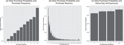
Note. The y axis represents the average daily purchase probability with 95% confidence intervals, conditional on a household’s prior purchase frequency, recency, or same-day ad exposures.
4.2. Ad Response Model
Building on the data described earlier, we specify a household-daily ad response model to quantify the effect of linear TV advertising on focal brand purchases. Let denote whether household i makes a purchase on day t () or not (). The purchase probability is determined by the utility that household i derives from purchasing from the focal brand on day t:
The ad stock is specified as
In Equation (9), and are household specific and time varying, capturing household i’s baseline purchase propensity and ad responsiveness on day t. We model them as
We allow and to vary by , a vector of observed, time-invariant household characteristics; includes average TV viewing time, focal brand ad and targeted show completion rates, and the allocation of TV viewing time across show genres (e.g., sports, reality, news) and dayparts (e.g., daytime, prime time, weekends).11 All elements of are calibrated using data from the month preceding the study period and are standardized to have a mean of zero and a standard deviation of one.12
To capture unobserved time-invariant heterogeneity in baseline purchase propensity and ad responsiveness, and are assumed to follow a bivariate normal distribution with correlation : .
In Equations (12) and (13), denotes purchase frequency (i.e., number of past purchases) and denotes purchase recency (i.e., number of days since last purchase).13 The indicator function equals one if household i has made at least one prior purchase before day t, allowing both baseline purchase propensity and ad responsiveness to differ between prospective and existing customers. For converted households (i.e., ), we allow and to evolve as functions of purchase frequency and recency, represented by and , respectively. The inclusion of log- and squared-log terms in allows both baseline purchase propensity and ad responsiveness to vary nonlinearly with purchase frequency and recency.14
4.3. Operationalization and Validation of the Proposed IV
4.3.1. Diagnostic Checks on Identifying Assumptions.
The validity of our proposed instrument depends on two identifying assumptions outlined in Section 3.2. The first is that the exact time at which a focal brand ad airs within a targeted show is quasi-randomly assigned by the network broadcasting the show. This assumption aligns with prevailing industry practices: In the United States, networks typically sell linear TV ad slots based on the show and airing date, schedule these slots approximately 7–10 days in advance (Bollapragada and Garbiras 2004), and implement an equitable rotation of advertisers’ ads across slots within a show to ensure fairness (Wilbur et al. 2013, McGranaghan et al. 2022).
In our empirical application, we assess the quasi-random ordering assumption by comparing within-show ad airing times for the focal brand versus nonfocal brands across targeted networks. As an illustration, Figure 2 presents the distributions of focal and nonfocal brand ad airing times across shows on MTV, a major network targeted by the focal brand.
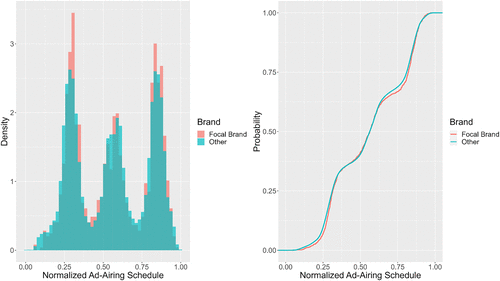
Note. Within-show ad airing times are normalized by show duration, where zero denotes the start and one denotes the end.
The within-show airing times for focal and nonfocal brand ads exhibit nearly identical distributions in both the PDFs and cumulative density functions (CDFs). MTV appears to schedule both focal and nonfocal brand ads according to a trimodal distribution. The Kolmogorov-Smirnov test confirms that the two distributions are statistically indistinguishable (p = 0.545), indicating that MTV scheduled focal brand ads in a manner comparable to other advertisers. Extending this analysis to all major networks (see Online Appendix E.2) yields similar results, with no significant differences in timing distributions between focal and nonfocal brand ads. These findings suggest that potential violations of the quasi-random ordering assumption are minimal in our setting.
The second identifying assumption, nonstrategic viewership, requires that a household’s viewership of a targeted show be independent of the within-show airing time of the focal brand ad. This assumption implies that households do not watch or skip the focal brand ad in a systematically different manner than they do ads of other brands.
At first glance, this may appear to be a relatively strong assumption, because households could, in principle, adjust their viewing behavior—watching or skipping—based on when the focal brand ad airs, implying that treatment might influence which segments of the show are viewed. However, in our empirical setting, 95.5% of focal brand ad exposures were watched in their entirety by treated households.15 This completion rate is statistically indistinguishable from that of nonfocal brand ads (95.7%, p = 0.12). Moreover, focal brand ad completion rates are highly consistent across household types: 95.5% for converted households and 95.6% for unconverted households (p = 0.20).
These uniformly high completion rates indicate that the risk of focal brand–specific strategic ad-skipping behavior is minimal in our context. Taken together, the evidence supports the plausibility of both identifying assumptions and provides empirical justification for estimating a household’s probability of focal brand ad exposure within a targeted show based on its observed show viewership.
4.3.2. Operationalizing the Proposed IV.
With both identifying assumptions passing their respective diagnostic checks, we now operationalize the proposed IV. Recall from Equation (8) that our household-show-level instrument is defined as . Although (i.e., whether household i is exposed to a focal brand ad within show s) and (i.e., whether show s is targeted by the focal brand) are directly observable in our data, constructing requires estimating —the probability that household i is exposed to a focal brand ad during show s in the event the show is targeted.
Recall from Equation (6) that . Because is directly observable from household TV viewing data, operationalizing requires specifying , which denotes the density function used by the network broadcasting show s to draw the within-show airing time of the focal brand ad. Under the quasi-random ordering assumption, the same density function governs the timing of all within-show ad placements, regardless of advertiser identity.
Accordingly, we operationalize as the normalized histogram of within-show ad placements observed for the network broadcasting show s; the left panel of Figure 2 shows a representative example. Under this operationalization, the estimate has an intuitive interpretation: It is the proportion of within-show ad placements that fall within household i’s viewing segment(s), .
With this setup, we next describe the implementation procedure in detail. Specifically, we nonparametrically estimate —household i’s probability of exposure to the focal brand’s ad within show s, conditional on the focal brand targeting the show—in three steps.
Step 1: Constructing the network-specific ad airing time distribution. We discretize within-show time at the second level and normalize each show’s duration to an interval from zero (beginning) to one (end), defining an ad’s airing time as the proportion of the show that has elapsed before the ad appears. For instance, an ad inserted at the 15th minute of a 30-minute show corresponds to a normalized ad airing time of 0.5.
Using all ad airings of all brands, we construct the empirical PDF of within-show ad airing times for each targeted network. These empirical PDFs provide estimates of , which governs the within-show ad airing time distribution for show s broadcast by network , where represents the normalized time within the show.
The left panel of Figure 3 visualizes our estimate of for MTV, a representative targeted network in our data. The focal brand’s ad airing times follow a trimodal distribution, with concentrations just after the first and second quarters of a show and immediately before the end of the show.
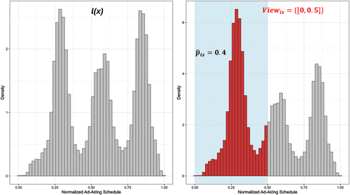
Notes. The x axis represents normalized show duration from zero (beginning) to one (end), and the y axis represents the probability density of an ad airing. (Right) Shaded area denotes the portion of the show that was viewed (), and the dark bars illustrate the calculation of estimated within-show focal brand ad exposure probability ().
Step 2: Identifying household show viewing patterns. Next, we map each household’s actual viewership of each targeted show onto the normalized show duration, based on second-by-second TV viewing data provided by LGADS. For example, if household i watched the first 15 minutes of a 30-minute show s, then . This is illustrated in the right panel of Figure 3, where the shaded area represents the portion of the show that was viewed.
Step 3: Computing the within-show probability of focal brand ad exposure. Conditional on the observed household show viewership , and the estimated targeted network’s ad airing time PDF , our estimate of , denoted by , can be expressed as .
The shaded bars in the right panel of Figure 3 visualize the calculation of : The red AUC represents our nonparametric estimate of for a household that watched the first half of a targeted show on MTV. In this example, the red AUC accounts for 40% of the total AUC, indicating a 40% probability that the household could be exposed to the focal brand’s ad, given and .
For each household i and show s, given , we compute the household-show–level IV as . In the illustrative example shown in Figure 3, when household i is actually exposed to the focal brand ad, and when the household is unexposed. The expected value of this IV is therefore .
Because focal brand purchases are observed at the daily level, we aggregate the household-show–level IV across all shows broadcast on day t to obtain the household-day–level IV: .
As noted in Section 3.3, a key property of our household-show–level IV is that it is nonzero only when a household partially watches a targeted show. This implies that our identification strategy relies on variation in ad exposure status among observations where households watch targeted shows without completing them in full. In our data, among households that watched at least one targeted show during the study period, only 1.8% completed all the targeted shows they watched (i.e., “always completers”), whereas the remaining 98.2% watched at least one targeted show partially.
Moreover, at the household-show level, only 7.6% of observations correspond to fully completed shows, whereas 51.1% lasted less than 10% of the show’s duration, 33% lasted between 10% and 90%, and the remaining 8.3% lasted between 91% and 99%.
Taken together, the small share of always completers (1.8%) and the large portion of partially completed household-show observations (92.4%) suggest that our identification strategy benefits from ample nonzero, network-induced exogenous shocks. This ensures sufficient statistical power to estimate the average treatment effect for the general population of smart TV households.16
4.3.3. Summary Statistics of Operationalized IV and Falsification Checks.
Table 2 presents summary statistics for the realized treatment , expected treatment , and the instrument across all household-show observations in which a household watched any portion of a targeted show (i.e., and ). Table 2 also reports summary statistics for the corresponding household-day-level aggregates, that is, , , and .
|
Table 2. Summary Statistics of Realized Ad Exposure, Expected Ad Exposure, and IV
| Mean | Standard deviation | 5% | 25% | 50% | 75% | 95% | |
|---|---|---|---|---|---|---|---|
| Household-show level | |||||||
| Realized ad exposure () | 0.29 | 0.45 | 0.00 | 0.00 | 0.00 | 1.00 | 1.00 |
| Expected ad exposure () | 0.29 | 0.38 | 0.001 | 0.01 | 0.06 | 0.56 | 1.00 |
| Proposed IV () | −0.002 | 0.25 | −0.38 | −0.04 | −0.004 | 0.00 | 0.49 |
| Household-day level | |||||||
| Realized ad exposure () | 0.51 | 0.84 | 0.00 | 0.00 | 0.00 | 1.00 | 2.00 |
| Expected ad exposure () | 0.51 | 0.77 | 0.00 | 0.01 | 0.15 | 0.82 | 2.00 |
| Proposed IV () | −0.004 | 0.39 | −0.61 | −0.11 | −0.01 | 0.00 | 0.75 |
Note. Summary statistics are based on 41,407,672 household-show–level and 23,985,341 household-day–level observations in which households watched any portion of a targeted show.
At the household-show level, the mean of closely aligns with the mean of , indicating that our estimate of expected treatment is unbiased. This, in turn, yields a household-show–level with a mean close to zero (−0.002). A similar pattern emerges at the household-day level, where the mean of , the mean of , and the mean of . These results indicate that both and pass the mean-zero falsification check discussed in Section 3.3.
Conceptually, our estimate of expected treatment, , resembles a propensity score. However, unlike traditional propensity score estimation, which typically involves calibrating a predictive model using the realized treatment status (in our case, ) as the dependent variable, we obtain nonparametrically and without reference to . This fundamentally different approach to expected treatment or propensity score estimation underscores that achieving equality between the means of and is nontrivial and not mechanically guaranteed.
Moreover, , indicating that our expected treatment estimate is highly correlated with the realized treatment, as expected. Most notably, , , , and . These results indicate that our instrument simultaneously satisfies two key conditions: (a) It is strongly correlated with the realized treatment, thereby meeting the relevance condition consistent with Proposition 1, and (b) it exhibits near-zero correlation with the show-targeting decision (), the estimated probability of focal brand ad exposure within a targeted show (), and the expected treatment estimate (), thereby passing the falsification checks on exogeneity consistent with Proposition 2.
Statistically, achieving both (a) and (b) is nontrivial: It requires that two highly correlated variables— and —yield a difference, , that is highly correlated with one () but uncorrelated with the other (). In Online Appendix E.3, we further compare the correlations in focal brand ad exposures with the correlations in network-induced shifters across targeted shows, providing additional support for the validity of the proposed IV.
At the household-day level, we observe a similar pattern: , , , , and . These results confirm that our household-day–level instrument likewise satisfies the relevance condition and passes the falsification checks on exogeneity.
4.4. Control Function Approach
Because each household’s daily purchase decision is modeled as a discrete choice (Equations (9) and (10)), we incorporate the proposed instrument into the ad response model using the control function approach (Petrin and Train 2010, Wooldridge 2015, Ebbes et al. 2016).
In the first stage, we regress each household’s daily focal brand ad exposures on its instrument and other variables that enter the utility function:
We retain the residual from the first-stage regression, denoted by , and include it in the second stage to correct for potential endogeneity bias in the ad response model. To align with the ad stock formulation of household daily focal brand ad exposures (i.e., ), we construct a corresponding “control function stock,” denoted by :
Taken together, in the second stage of the control function approach, we estimate a probit model in which enters the utility function as an additional control:
5. Results
5.1. Evidence of Bias Correction by the Proposed Identification Strategy
The first-stage regression results (Equations (16) and (17)), reported in Table 3, confirm that has the expected positive and statistically significant effect on focal brand ad exposure ( = 0.970, p < 0.01). The instrument is also highly relevant, as evidenced by a univariate F-statistic of 1,902,996 (p < 0.001). Variables related to purchase history, such as frequency, recency, and the first-month postconversion promotion indicator, are uncorrelated with focal brand ad exposure once we condition on . Although competitors’ ad spend is positively associated with focal ad exposure, the effect size is negligible: A one-standard-deviation increase corresponds to only 0.008 additional focal brand ad exposures.
|
Table 3. Parameter Estimates from the First-Stage Model
| Model component | Parameter | Estimate | Standard error | ||
|---|---|---|---|---|---|
| Intercept | 0.060*** | 0.001 | |||
| 0.970*** | 0.001 | ||||
| Postconversion | 0.005 | 0.004 | |||
| Frequency (log) | 0.0003 | 0.003 | |||
| Frequency (log) squared | −0.0003 | 0.002 | |||
| Recency (log) | −0.002 | 0.003 | |||
| Recency (log) squared | 0.0001 | 0.001 | |||
| First month postconversion promotion | −0.001 | 0.002 | |||
| Competitor ad spend | 0.008*** | 0.0004 | |||
| Month fixed effects | — | Yes | |||
| Day-of-week fixed effects | — | Yes | |||
| Holiday fixed effects | — | Yes | |||
| Household characteristics | Yes | ||||
| Standard deviation of random intercept | 0.012*** | 0.001 | |||
Note. The DV is daily household focal brand ad exposures .
***p < 0.01; **p < 0.05; *p < 0.1.
The second-stage household-daily ad response model is specified as a random-coefficient probit estimated using simulated maximum likelihood (SML) with Halton draws (Train 1999). To assess how key parameter estimates vary across specifications, we also estimate several simplified versions for comparison. The results are reported in Table 4.
|
Table 4. Second-Stage Estimation Results for the Ad Response Model
| Parameter | No carryover or moderation effects without CF (1) | No carryover or moderation effects with CF (2) | No moderation effects without CF (3) | No moderation effects with CF (4) | Full model without CF (5) | Full model with CF (6) | |||||||
|---|---|---|---|---|---|---|---|---|---|---|---|---|---|
| Estimate | Standard error | Estimate | Standard error | Estimate | Standard error | Estimate | Standard error | Estimate | Standard error | Estimate | Standard error | ||
| Intercept | −3.338*** | 0.005 | −3.368*** | 0.005 | −3.370*** | 0.005 | −3.368*** | 0.006 | −3.430*** | 0.006 | −3.429*** | 0.006 | |
| Ad Stock | 0.023*** | 0.003 | 0.010* | 0.005 | 0.016*** | 0.002 | 0.007** | 0.003 | 0.018*** | 0.003 | 0.012*** | 0.003 | |
| Control Function | — | — | 0.015** | 0.007 | — | — | 0.003*** | 0.001 | — | — | 0.003*** | 0.001 | |
| Post Conversion | 1.611*** | 0.010 | 1.611*** | 0.010 | 1.611*** | 0.010 | 1.611*** | 0.009 | 1.499*** | 0.012 | 1.498*** | 0.013 | |
| Frequency (log) | 0.516*** | 0.007 | 0.516*** | 0.007 | 0.516*** | 0.007 | 0.516*** | 0.007 | 0.459*** | 0.008 | 0.459*** | 0.008 | |
| Frequency (log) sq. | −0.045*** | 0.003 | −0.045*** | 0.003 | −0.045*** | 0.003 | −0.045*** | 0.003 | −0.061*** | 0.003 | −0.061*** | 0.003 | |
| Recency (log) | −0.120*** | 0.006 | −0.120*** | 0.006 | −0.120*** | 0.006 | −0.120*** | 0.006 | −0.103*** | 0.008 | −0.103*** | 0.008 | |
| Recency (log) sq. | −0.027*** | 0.001 | −0.027*** | 0.001 | −0.027*** | 0.001 | −0.027*** | 0.001 | −0.028*** | 0.002 | −0.028*** | 0.002 | |
| Adstock Post Conversion | — | — | — | — | — | — | — | — | 0.001 | 0.013 | 0.004 | 0.013 | |
| Ad Stock Freq (log) | — | — | — | — | — | — | — | — | 0.017* | 0.009 | 0.019* | 0.009 | |
| Ad Stock Freq (log) sq. | — | — | — | — | — | — | — | — | −0.010* | 0.005 | −0.010* | 0.005 | |
| Ad Stock Rec (log) | — | — | — | — | — | — | — | — | −0.011 | 0.011 | −0.011 | 0.011 | |
| Ad Stock Rec (log) sq. | — | — | — | — | — | — | — | — | 0.004** | 0.002 | 0.004** | 0.002 | |
| First Month Post-Conversion Promotion | 0.200*** | 0.005 | 0.200*** | 0.006 | 0.200*** | 0.005 | 0.200*** | 0.005 | 0.189*** | 0.006 | 0.189*** | 0.006 | |
| Competitor Ad Spend | 0.014*** | 0.005 | 0.014*** | 0.004 | 0.014*** | 0.005 | 0.014*** | 0.006 | 0.014** | 0.005 | 0.014*** | 0.005 | |
| Month fixed effects | — | Yes | Yes | Yes | Yes | Yes | Yes | ||||||
| Day-of-week fixed effects | — | Yes | Yes | Yes | Yes | Yes | Yes | ||||||
| Holiday fixed effects | — | Yes | Yes | Yes | Yes | Yes | Yes | ||||||
| Carryover | 0/0 | 0/0 | 0.7/0 | 0.7/0.95 | 0.7/0 | 0.7/0.95 | |||||||
| Household characteristics | Yes | Yes | Yes | Yes | Yes | Yes | |||||||
| HH characteristics Adstock | — | — | — | — | Yes | Yes | |||||||
| Standard deviation (intercept) | — | — | — | — | 0.197*** | 0.004 | 0.198*** | 0.005 | |||||
| Standard deviation (Adstock) | — | — | — | — | 0.003 | 0.015 | 0.015 | 0.012 | |||||
| Rho | — | — | — | — | −0.553 | 0.446 | −0.538 | 0.351 | |||||
Notes. Columns (1) and (2) assume no carryover of ad effects, no evolution of ad responsiveness, and no unobserved heterogeneity. Columns (3) and (4) assume no evolution of ad responsiveness and no unobserved heterogeneity. Columns (5) and (6) incorporate all model components. Estimates in Columns (2), (4), and (6) are obtained using the control function approach, with standard errors derived from 50 bootstrapped samples.
***p < 0.01; **p < 0.05; *p < 0.1.
Columns 1 and 2. Column 1 reports the simplest specification, which assumes no ad carryover (), no control function ( and ), no moderation of ad responsiveness by time-invariant household characteristics () or purchase history (), and no unobserved heterogeneity in baseline purchase propensity or ad responsiveness (, , and ). Column 2 extends this baseline by introducing a control function term, allowing to be estimated while fixing the decay parameter , such that .
The ad effect estimate () declines from 0.023 (p < 0.01) in column 1 to 0.010 (p < 0.1) in column 2, highlighting the debiasing effect of the control function term . The positive and significant coefficient for (, p < 0.05) further confirms that households’ daily ad exposures are endogenous, exhibiting positive spurious correlation with households’ daily purchase decisions.
Columns 3 and 4. Columns 3 and 4 extend columns 1 and 2, respectively, by allowing the daily decay parameters in and (i.e., and ) to be empirically determined via a grid search (Danaher et al. 2020, Shapiro et al. 2021, Tsai and Honka 2021). Rather than imposing equality between and , we vary them independently from 0 to 0.99 in increments of 0.05 and select the combination that maximizes out-of-sample fit, yielding and .17 This pair is then held fixed when comparing models with or without the control function term and with or without random effects.
The control function term remains positive and significant (, p < 0.01).18 Comparing the estimates in columns 3 and 4, we observe that including reduces the estimated ad effect by more than 50%, from (p < 0.01) to (p < 0.05). The continued significance of the coefficient (, p < 0.01) reinforces the presence of endogeneity, consistent with the pattern observed in the comparison between columns 1 and 2.
Columns 5 and 6. Columns 5 and 6 further extend columns 3 and 4 by allowing ad responsiveness to vary with household characteristics () and purchase history (), as well as by incorporating unobserved heterogeneity in both baseline purchase propensity and ad responsiveness (, , and ). Once again, inclusion of the control function term corrects for substantial upward bias in the naïve ad effect estimate, as evidenced by the decline in from 0.018 (p < 0.01) in column 5 to 0.012 (p < 0.01) in column 6.19
For an average unconverted household, the baseline daily conversion rate is 0.012%. The naïve ad effect estimate suggests that a single focal-brand ad exposure lifts this rate by approximately 7.5%, whereas the endogeneity-corrected estimate from our proposed model yields a smaller but still significant lift of 4.6%. For the remainder of the paper, we focus on the endogeneity-corrected estimates from the full model (column 6 of Table 4).
To situate our estimates within the literature, we compute short- (same-day) and long-term (30-day) ad elasticities for the average panel household. Elasticities are defined as the percentage change in purchase incidence over the same day (30 days) in response to a 1% change in ad stock. After correcting for endogeneity, the short- and long-term elasticities are 0.045 and 0.143, respectively, compared with 0.072 and 0.222 without correction—an overstatement of 55%. These naïve elasticities closely align with the mean short- and long-term elasticities of 0.12 and 0.24 reported by Sethuraman et al. (2011), highlighting the risk of substantially inflated estimates when endogeneity is not properly addressed.20
5.2. Baseline Purchase Propensity and Purchase History
The estimates in column 6 of Table 4 capture how a household’s baseline purchase propensity evolves with its purchase history. Following the first purchase, baseline propensity rises sharply ( = 1.498, p < 0.01), corresponding to an increase in daily purchase probability from 0.012% for an unconverted household to 1.5% for a newly converted household.
One likely explanation for this increase is the initial setup cost associated with using the focal brand’s platform. Before placing their first order, households must download the app (or access the website), create an account, and enter a payment method. Because these steps are not required for subsequent purchases, the reduction in transaction friction naturally leads to a higher baseline purchase propensity after the first purchase.
Among converted households, prior purchase frequency has a positive but diminishing effect on baseline purchase propensity ( = 0.459, p < 0.01; = −0.061, p < 0.01), consistent with self-reinforcing habit formation, particularly during the early stages of repeat purchasing. In contrast, baseline purchase propensity declines with increasing recency ( = −0.103, p < 0.01; = −0.028, p < 0.01), indicating that households become less likely to repurchase the longer they wait, a pattern consistent with the recency-trap effect documented in other contexts (Neslin et al. 2013).
Taken together, these results show that baseline purchase propensity continues to evolve with purchase frequency and recency beyond the initial postconversion increase. For example, a household with one prior purchase has a 1.5% daily probability of making a purchase, which rises to 4.0% after three purchases and to 5.5% after five. Conversely, a household that purchased yesterday has a 1.5% probability of buying again today, which declines to 0.9% after one week and to 0.3% after four weeks.
5.3. Ad Responsiveness and Purchase History
We next examine how a household’s responsiveness to the focal brand’s TV ads varies with its purchase history, as captured by the estimates in column 6 of Table 4. Because is statistically insignificant (p > 0.1), there is no evidence that a household becomes either more or less responsive to the focal brand’s TV ads immediately following its trial purchase. To better interpret how ad responsiveness evolves with prior purchases, Figure 4 visualizes the nonlinear patterns implied by the estimates.
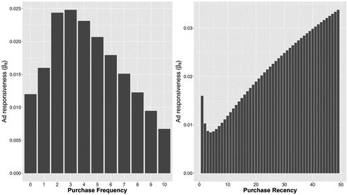
Note. The moderating effects of purchase frequency and recency on ad responsiveness () reveal an inverted U-shaped relationship with frequency and a U-shaped relationship with recency.
The left panel of Figure 4 shows an inverted U-shaped relationship between ad responsiveness and purchase frequency. Households are most responsive to the focal brand’s TV ads after two to four prior purchases—that is, during the early stages of repeat purchasing. Beyond this point, ad responsiveness declines as households become more frequent purchasers, reflecting a reduced impact of TV advertising on habitual buyers. In contrast, the right panel of Figure 4 depicts a U-shaped relationship between ad responsiveness and purchase recency. Households are least responsive to the focal brand’s TV ads approximately three to five days after a purchase.
These patterns are also reflected in the short-term ad elasticity estimates. For an average household with one prior purchase, same-day ad elasticity increases from 0.040 to 0.056 following the second purchase but declines to 0.046 after the fifth. Likewise, for a typical household with one prior purchase, same-day ad elasticity decreases from 0.040 to 0.027 one week after the last purchase but then rises to 0.078 four weeks later.
Although these results suggest that the focal brand’s TV ad effectiveness varies nonmonotonically with prior purchase frequency and recency, the underlying mechanisms remain unclear. Future research is needed to better understand the drivers of these dynamics. One plausible explanation is that, with each additional purchase, the effectiveness of TV ads may shift due to changes in their informational versus emotional roles (Tellis 1988; Deighton et al. 1994; Ackerberg 2001, 2003).
Regardless of the specific mechanisms, the complex dynamics of baseline purchase propensity and ad responsiveness with respect to purchase frequency and recency yield important managerial implications for behaviorally targeted TV advertising. First, to capture the full impact of TV ads, advertisers must account for state-dependence effects, such as habit formation acceleration and recency trap avoidance, in addition to same-day and carryover effects. Second, when formulating targeting strategies, advertisers should incorporate prior purchase frequency and recency as segmentation criteria (e.g., prospective versus existing customers, early repeat versus habitual purchasers, and recent versus lapsed purchasers). For instance, the focal brand may benefit from targeting lapsed households, those who have not purchased in an extended period, given their substantially higher ad responsiveness. However, because baseline purchase propensity declines sharply with increasing recency, timely intervention is crucial to prevent households from falling into a self-reinforcing recency trap. Effective behavioral targeting should therefore balance these opposing forces by accounting for both the decline in baseline purchase propensity and the rise in ad responsiveness as recency increases.
5.4. Household Heterogeneity and Other Control Variables
Table 5 presents parameter estimates capturing observed household heterogeneity in baseline purchase propensity and ad responsiveness. Households that watch more TV generally exhibit lower baseline purchase propensities, likely because heavy TV viewers tend to be older and less engaged with food delivery services. In contrast, households with higher sports viewership display higher baseline purchase propensities, consistent with sports audiences skewing younger—a demographic more inclined to adopt food delivery. Conversely, heavy news viewers, who also skew older, appear more reliant on traditional meal preparation and therefore show a lower likelihood of using digital food ordering services.
|
Table 5. Parameter Estimates for Observed Household Heterogeneity
| Baseline purchase propensity () | Ad responsiveness () | |||
|---|---|---|---|---|
| Estimate | Standard error | Estimate | Standard error | |
| Average TV viewing | −0.019*** | 0.002 | −0.004** | 0.002 |
| Sports viewing | 0.014*** | 0.002 | 0.004* | 0.002 |
| Reality viewing | −0.003* | 0.002 | 0.003 | 0.002 |
| News viewing | −0.012*** | 0.002 | 0.002 | 0.002 |
| Daytime viewing | −0.006** | 0.002 | −0.001 | 0.003 |
| Prime time viewing | −0.011*** | 0.002 | 0.001 | 0.003 |
| Weekend viewing | −0.005** | 0.002 | −0.0004 | 0.003 |
| Ad completion | 0.001 | 0.001 | −0.004 | 0.003 |
| Show completion | 0.003** | 0.001 | 0.003 | 0.002 |
Note. The standard errors are derived from 50 bootstrapped samples.
***p < 0.01; **p < 0.05; *p < 0.1.
We also find that households with greater sports viewership are more responsive to the focal brand’s TV ads. In contrast, heavy TV viewers exhibit lower ad responsiveness, possibly due to ad saturation: greater exposure to a wide range of advertisers may lead to ad fatigue and reduced attention to any single advertiser, including the focal brand.
These observed heterogeneities are economically meaningful. For instance, a one-standard-deviation increase in a typical household’s sports viewership raises short-term ad elasticity from 0.045 to 0.061, whereas a one-standard-deviation increase in overall TV viewing reduces it from 0.045 to 0.030.
Beyond observed heterogeneities, column 6 of Table 4 also reveals substantial unobserved heterogeneity in baseline purchase propensity ( = 0.156, p < 0.01). However, unobserved heterogeneity in ad responsiveness is not statistically significant, nor is there evidence of a significant correlation between unobserved baseline purchase propensity and ad responsiveness.
Lastly, we examine the effects of two key control variables. The first-month postconversion promotion, available exclusively to new customers, has a positive and significant effect (, p < 0.01), corresponding to a 58% increase in daily purchase probability. Competitor ad spend likewise exerts a positive and significant influence on focal brand purchase propensity (, p < 0.01). The implied same-day competitor ad elasticity is 0.016 for unconverted households, approximately 36% of the focal brand’s own same-day ad elasticity.
This finding aligns with prior research documenting positive spillover effects from competitor TV advertising. For example, Anderson and Simester (2013) and Sahni (2016) report such spillovers in field experiments, whereas Du et al. (2019) find that immediate TV ad elasticity of brand search ranges from 0.02 to 0.22 for own-brand ads and from 0.003 to 0.05 for competitor ads. Consistent with these studies, our results suggest that competitor TV ads can indirectly benefit the focal brand, potentially because the category expansion effect outweighs the share-stealing effect in a relatively young industry.
6. Concluding Remarks
The widespread adoption of ACR-enabled smart TVs and STBs has made second-by-second TV viewing data available to networks and advertisers at unprecedented scales. These high-granularity, large-scale audience measurement data are emerging as a viable contender for TV ad currency. When merged with first-party CRM data, modern single-source data have the potential to transform the landscape of TV advertising—not only by enabling improved targeting and attribution in practice but also by fostering methodological innovation in marketing science.
This research contributes to such methodological advancement by developing a novel IV for estimating the causal effect of linear TV advertising using household-level observational data. Our method addresses a central challenge in ad effectiveness research based on such data: the lack of a generalizable causal identification strategy that is robust to both targeting and activity biases. The key insight underlying our approach is that, in linear TV—where ad buys are primarily targeted at the show level—networks typically assign within-show ad slots across advertisers in a quasi-random manner. This practice introduces stochastic variation in realized ad exposure among households that watch only part of a targeted show.
Through formal proofs, a stylized numerical example, and an empirical application, we show that, under the identifying assumptions, there exists exogenous, network-induced variation in household-show-level linear TV ad exposures that can be leveraged for causal identification. The core innovation of our method lies in showing how this exogenous variation can be extracted nonparametrically—as the residual between a household’s realized ad exposure and its expected treatment—and used as an instrument at either the household-show or household-day level. A notable feature of this approach is that the expected treatment is estimated without fitting a predictive model using the realized treatment as the dependent variable, distinguishing it from traditional propensity score-based methods.
For IV-based identification, instrument exogeneity is inherently untestable in real-world applications. Nevertheless, a key advantage of our IV construction approach is that it enables multiple empirical checks to assess the credibility of both the identifying assumptions and the instrument itself.
Quasi-random ordering assumption: Examine whether the empirical distribution of within-show ad airing times for the focal brand is statistically indistinguishable from that of nonfocal brands. Passing this check increases confidence that networks assign within-show ad slots for the focal brand through a quasi-random process similar to that used for other advertisers.
Nonstrategic viewership assumption: Examine whether ad-skipping rates for the focal brand are comparable to those for nonfocal brands. Passing this check—particularly when ad-skipping rates are low (e.g., <4.5%, as in our data)—increases confidence that viewers do not avoid focal brand ads in a systematically different manner than they do ads of other brands.
Instrument validity: Examine whether the constructed IV (a) has a mean close to zero, ensuring the expected treatment estimate is unbiased, (b) is strongly and positively correlated with realized treatment, satisfying the relevance condition; and (c) is uncorrelated with the expected treatment estimate, thereby passing the falsification check for exogeneity.
With respect to practical effectiveness, our empirical results show that omitting the proposed IV correction for endogeneity leads to naïve ad elasticity estimates overstated by 55%, even after controlling for a rich set of covariates and incorporating random effects for both baseline purchase propensity and ad responsiveness. This substantial bias correction underscores the value of our method for achieving credible causal inference in observational TV advertising research.
Substantively, in the context of food delivery services, we find that baseline purchase propensity rises sharply after the initial purchase and continues to increase with each subsequent purchase, albeit at a diminishing rate—a pattern of positive reinforcement consistent with habit formation. We also observe a recency trap effect: Baseline purchase propensity declines steadily with each additional day without a purchase. Moreover, ad responsiveness varies systematically with past purchase behavior. Early repeat purchasers (those with two to four prior purchases) exhibit the highest responsiveness to the focal brand’s TV ads. With respect to purchase recency, ad responsiveness initially declines immediately following a purchase but subsequently rebounds as more time elapses without another purchase.
As modern single-source data, such as those employed in this study, become increasingly available, our identification approach offers a portable solution for marketing researchers, advertisers, and policymakers seeking to measure TV ad effectiveness using household-level observational data. Although RCTs are often costly, logistically challenging, or infeasible in the linear TV context, our method provides a practical and cost-efficient alternative, enabling robust causal inference at scale by leveraging the quasi-random ordering of within-show ad placements inherent to linear TV advertising.
Several boundary conditions of our identification strategy warrant future extension. First, the quasi-random ordering assumption may not hold in contexts where advertisers prenegotiate specific ad positions or where networks employ addressable technologies that adjust ad timing based on viewer characteristics. Second, the assumption of nonstrategic viewership may be violated if the focal advertiser elicits systematically different viewing behaviors (e.g., viewers are uniquely inclined to attend to or skip its ads). Third, although our identification strategy addresses the two primary sources of endogeneity—targeting and activity biases—other sources may persist (e.g., advertisers strategically tailor ad copy or campaign objectives based on show audience characteristics). Future research could extend our framework to accommodate these complexities.
All in all, we hope our study encourages further exploration of the full potential of large-scale, high-granularity single-source data. As the history of marketing science demonstrates, each wave of audience measurement innovation has spurred advances in empirical methods and scientific discovery (Du et al. 2021). We view our work as part of this ongoing evolution, providing a methodological foundation for future research on the causal effects and effectiveness of TV advertising.
The authors thank Ken Wilbur, Linli Xu, Max Joo, Sesh Tirunillai, Kathy Li, Jason Duan, Liye Ma, Samsun Knight, and the Marketing Science review team for thoughtful comments and suggestions and participants at Advertising Research Foundation Attribution & Analytics Accelerator 2022, Marketing Science Conference 2023, Interactive Marketing Research Conference 2024, Marketing Dynamics Conference 2024, and seminar participants at Amazon Ads, Dartmouth College, Indiana University Bloomington, London Business School, Northeastern University, Oklahoma State University, Western University, University of Arizona, University of Florida, University of Illinois Chicago, University of Illinois Urbana-Champaign, and University of Miami for feedback. This research was initiated while all authors were at the University of Houston, and the authors gratefully acknowledge the early support of Ed Blair and the Marketing Department at the Bauer College of Business.
1 With the advent of automatic content recognition (ACR) technology and the widespread adoption of ACR-enabled smart TVs and set-top boxes (STBs), providers such as Comscore, iSpot, and LG Ad Solutions now collect second-by-second TV viewership data from tens of millions of households (NBCUniversal 2022). When such granular TV viewing data from large-scale panels are merged with advertisers’ first-party response data (e.g., via meshed IP-address matching), they produce what we term modern single-source data.
2 LGADS collects TV viewing data through ACR technology from more than 35 million opt-in smart TVs in the United States, spanning TV brands such as LG, Seiki, Skyworth, RCA, and Askey. Retrieved on August 19, 2024 from https://lgads.tv/tv-data/.
3 Most prior studies using household-level data have not explicitly addressed the endogeneity of TV ad exposure. Notable exceptions include Lodish et al. (1995) and Hu et al. (2007), who employ split-cable field experiments, and Tuchman et al. (2018), who use a simultaneous equation model to account for endogenous ad-skipping behavior.
4 This pattern is evident in our empirical setting. Our model estimates indicate a daily carryover of approximately 0.7, which is substantially lower than the weekly carryover of 0.9 (equivalent to a daily carryover of 0.985) reported in prior studies of CPGs (Shapiro et al. 2021).
5 Observed household characteristics, together with random or fixed household effects, can be included as controls when both a household’s preference for targeted shows and its baseline demand for the focal brand are correlated with these characteristics. Likewise, observed temporal factors, along with random or fixed time effects, can be included to account for time-varying unobservables that influence all households in a similar manner.
6 For ease of exposition, we treat as a point rather than an interval.
7 In Section 4.3, we demonstrate how can be obtained nonparametrically and present descriptive statistics of the proposed instruments in our empirical setting, along with supporting evidence of their validity.
8 Although each order is linked to a device ID, the data do not distinguish between mobile app and web browser transactions. According to the data provider, however, the majority of orders were placed through mobile apps.
9 Online Appendix D presents additional hour-of-the-week distributions of purchases and ad exposures.
10 We account for the top two competitors’ TV advertising by acquiring DMA-day-level TV ad spend data from Kantar. Specifically, we calculate competitive ad spend per capita for each DMA-day and include it as a control variable in the ad response model.
11 The ad completion rate is defined as the total duration of the focal brand’s ads watched by a household divided by the total length of all focal brand ads encountered by that household (with at least one second of exposure). The targeted show completion rate is defined as the total duration of targeted shows watched by a household divided by the total length of all targeted shows it encountered (with at least one minute of exposure).
12 We do not have access to demographic variables such as age and gender due to the data provider’s data-sharing policy. Instead, we use households’ show-viewing behavior from the month preceding the study period as a proxy for time-invariant household characteristics.
13 In the CRM literature, in addition to recency (R) and frequency (F), total monetary value (M) is often found to be a strong predictor of an existing customer’s future purchase behavior. However, because frequency and total monetary value are highly correlated in our data, we focus exclusively on recency and frequency in this study.
14 We compare four specifications in Online Appendix E.1: (1) linear, (2) linear + squared, (3) log, and (4) log + squared-log. The log + squared-log specification outperforms the other three based on log-likelihood, AIC, and BIC.
15 In our empirical implementation, a household is considered treated if it is exposed to any part of a focal brand ad, regardless of the duration of the exposure.
16 Our identification strategy may lead to a downward bias in the estimated ad effects if households that consistently watch entire shows are also more responsive to TV ads.
17 For each decay parameter combination, we estimate the ad response model using data from the first 120 days of the study period and evaluate the model’s log-likelihood on data from the remaining 13 days.
18 The correlation between and is 0.72. To assess potential multicollinearity, we calculate the variance inflation factors (VIFs) for and in the second-stage model, which are 2.42 and 2.27, respectively—well below the conventional threshold of 10.
19 As a robustness check of the identified positive effect of linear TV advertising, we conduct a placebo test by replacing the focal brand’s ad exposures with those from a major automobile manufacturer and re-estimating the proposed model. The null effect of auto ads on household purchases of the focal brand suggests that the identified positive effect of focal brand ads is unlikely to be coincidental (see Online Appendix E.4 for details).
20 Our endogeneity-corrected long-term elasticity of 0.143 remains notably higher than the 0.023 reported by Shapiro et al. (2021), likely reflecting differences in brand maturity. Shapiro et al. (2021) primarily examine mature brands, for which prior research consistently documents lower ad elasticities (Sethuraman et al. 2011).
References
- (2001) Empirically distinguishing informative and prestige effects of advertising. RAND J. Econom. 32(2):316–333.Crossref, Google Scholar
- (2003) Advertising, learning, and consumer choice in experience good markets: An empirical examination. Internat. Econom. Rev. 44(3):1007–1040.Crossref, Google Scholar
- (2013) Advertising in a competitive market: The role of product standards, customer learning, and switching costs. J. Marketing Res. 50(4):489–504.Crossref, Google Scholar
- (2004) Scheduling commercials on broadcast television. Oper. Res. 52(3):337–345.Link, Google Scholar
- (2008) Database paper—The IRI marketing data set. Marketing Sci. 27(4):745–748.Link, Google Scholar
- (2020) Advertising effectiveness for multiple retailer-brands in a multimedia and multichannel environment. J. Marketing Res. 57(3):445–467.Crossref, Google Scholar
- (1994) The effects of advertising on brand switching and repeat purchasing. J. Marketing Res. 31(1):28–43.Crossref, Google Scholar
- (2018) TV viewing and advertising targeting. J. Marketing Res. 55(1):99–118.Crossref, Google Scholar
- (2019) Immediate responses of online brand search and price search to TV ads. J. Marketing 83(4):81–100.Crossref, Google Scholar
- (2021) Capturing marketing information to fuel growth. J. Marketing 85(1):163–183.Crossref, Google Scholar
- (2016)
Dealing with endogeneity: A nontechnical guide for marketing researchers . Homburg C, Klarmann M, Vomberg A, eds. Handbook of Market Research (Springer, Cham, Switzerland), 30–31.Crossref, Google Scholar eMarketer (2022) Advanced TV 2022: What’s next for addressable, programmatic, and connected TV. Accessed April 12, 2025, https://www.emarketer.com/content/advanced-tv-2022#page-report.Google Scholar- (2023) Close enough? A large-scale exploration of non-experimental approaches to advertising measurement. Marketing Sci. 42(4):768–793.Link, Google Scholar
- (2019) A comparison of approaches to advertising measurement: Evidence from big field experiments at Facebook. Marketing Sci. 38(2):193–225.Link, Google Scholar
- (2021) Inefficiencies in digital advertising markets. J. Marketing 85(1):7–25.Crossref, Google Scholar
- (2017) Super bowl ads. Marketing Sci. 37(1):78–96.Link, Google Scholar
- (2007) An analysis of real world TV advertising tests: A 15-year update. J. Advertising Res. 47(3):341–353.Crossref, Google Scholar
- (2014) Television advertising and online search. Management Sci. 60(1):56–73.Link, Google Scholar
- (2023) TV advertising and online sales: A case study of intertemporal substitution effects for an online travel platform. J. Marketing Res. 61(2):248–270.Crossref, Google Scholar
- (2014) Online ads and offline sales: Measuring the effect of retail advertising via a controlled experiment on Yahoo!. Quant. Marketing Econom. 12(3):235–266.Crossref, Google Scholar
- (2011) Here, there, and everywhere: Correlated online behaviors can lead to overestimates of the effects of advertising. Proc. 20th Internat. Conf. World Wide Web (ACM, New York), 157–166.Google Scholar
- (2024) Preference externality estimators: A comparison of border approaches and IVs. Management Sci. 70(11):7892–7910.Link, Google Scholar
- (2015) Television advertising and online shopping. Marketing Sci. 34(3):311–330.Link, Google Scholar
- (1995) How T.V. advertising works: A meta-analysis of 389 real world split cable TV advertising experiments. J. Marketing Res. 32(2):125–139.Crossref, Google Scholar
- (2018) Understanding programmatic TV advertising. Internat. J. Advertising 37(5):769–784.Crossref, Google Scholar
- (2022) How viewer tuning, presence, and attention respond to ad content and predict brand search lift. Marketing Sci. 41(5):873–895.Link, Google Scholar
- (2021) How and when to use the political cycle to identify advertising effects. Marketing Sci. 40(2):283–304.Link, Google Scholar
NBC Universal (2022) Measurement framework look book V1. Report, NBC Universal, New York.Google Scholar- (2013) Overcoming the “recency trap” in customer relationship management. J. Acad. Marketing Sci. 41(3):320–337.Crossref, Google Scholar
- (2010) A control function approach to endogeneity in consumer choice models. J. Marketing Res. 47(1):3–13.Crossref, Google Scholar
- (2016) Advertising spillovers: Evidence from online field experiments and implications for returns on advertising. J. Marketing Res. 53(4):459–478.Crossref, Google Scholar
- (2011) How well does advertising work? Generalizations from a meta-analysis of brand advertising elasticity. J. Marketing Res. 48(3):457–471.Crossref, Google Scholar
- (2018) Positive spillovers and free riding in advertising of prescription pharmaceuticals: The case of antidepressants. J. Political Econom. 126(1):381–437.Crossref, Google Scholar
- (2021) TV advertising effectiveness and profitability: Generalizable results from 288 brands. Econometrica 89(4):1855–1879. Crossref, Google Scholar
- (2019) Ask your doctor? Direct-to-consumer advertising of pharmaceuticals. Rev. Econom. Stud. 86(2):836–881.Crossref, Google Scholar
- (2017) Super returns to Super Bowl ads? Quant. Marketing Econom. 15(1):1–28.Crossref, Google Scholar
- (1988) Advertising exposure, loyalty, and brand purchase: A two-stage model of choice. J. Marketing Res. 25(2):134–144.Crossref, Google Scholar
- (2020) Spillovers from mass advertising: An identification strategy. Marketing Sci. 39(4):807–826.Link, Google Scholar
- (1999) Halton sequences for mixed Logit. Working paper, Department of Economics, University of California, Berkeley.Google Scholar
- (2021) Informational and noninformational advertising content. Marketing Sci. 40(6):1030–1058.Abstract, Google Scholar
- (2018) Television ad-skipping, consumption complementarities and the consumer demand for advertising. Quant. Marketing Econom. 16(2):111–174.Crossref, Google Scholar
- (2013) Correcting audience externalities in television advertising. Marketing Sci. 32(6):892–912.Link, Google Scholar
- (2015) Control function methods in applied econometrics. J. Human Resources 50(2):420–445.Crossref, Google Scholar
- (2017) Online shopping and social media: Friends or foes? J. Marketing 81(6):24–41.Crossref, Google Scholar