Visual Plant Imagery and Property Valuation: A Descriptive Analysis
Abstract
Homebuyers increasingly rely on real estate websites to evaluate properties throughout the home purchase process. Although most property profile images display inanimate objects (e.g., walls and furniture), some display living objects such as plants. Informed by phytophilia theory, which proposes that humans have an innate attraction toward plant life, we examine whether online home profiles with more versus fewer images containing plant life differ systematically in property valuation. First, we report the results of a survey of real estate agents indicating that awareness and priority of plant usage are currently low. Then we conduct a descriptive analysis of a large representative sample of homes sold in the United States and find that online profiles with more plant images tend to have higher transaction prices (as well as faster transaction speeds and higher levels of online engagement). This difference persists after conditioning on factors related to property and neighborhood characteristics, home presentation characteristics in the images and texts, and marketplace conditions and expectations. The result is stronger for interior versus exterior images, for earlier- versus later-appearing images, and in geographic areas where the current use of plant images is less prevalent. Implications for future research are discussed.
History: Puneet Manchanda served as the senior editor.
Funding: This work was supported by a Social Sciences and Humanities Research Council of Canada Insight Development Grant.
Supplemental Material: The online appendix and data files are available at https://doi.org/10.1287/mksc.2025.0145.
1. Introduction
Homebuyers increasingly rely on real estate websites such as Zillow®, Trulia®, and Redfin® to view properties online throughout the home-buying process. It is reported that 97% of homebuyers search online for information while house hunting (National Association of Realtors 2021), with 89% stating that visual images of homes are very helpful in the decision-making process (Carrillo 2008, Luchtenberg et al. 2019). Thus, the way homes are visually presented on these platforms likely plays an important role in how much attention they attract from potential buyers, how appealing they are perceived to be, how quickly they sell, and the price buyers are willing to pay.
Whereas most home profile images display inanimate objects such as walls and furniture, some display plants, toward which humans have a natural affinity. According to phytophilia theory, humans have an innate tendency to affiliate with vegetative life forms such as plants and trees, because plant life has, over time, contributed to human well-being and survival (Wilson 1984, Joye and van den Berg 2011, Brengman et al. 2012, Tifferet and Vilnai-Yavetz 2017). Plant-containing images may thus draw a disproportionate share of attention and visually “pop out,” making home profiles more salient and memorable. It is therefore possible that home profiles with more plant-containing images are associated with more positive online engagement, faster transaction speeds, and higher prices paid.
In this research, we investigate several research questions with descriptive analyses. First, what is the current level of awareness and priority of plant usage among real estate agents? Second, do home profiles with more versus fewer plant images differ systematically in property valuation, and does this difference persist conditional on factors such as inherent property and neighborhood attributes, presentation efforts evident in profile images and texts, and latent market conditions or expectations? Third, is there heterogeneity in the strength of the association between plant images and property valuation as a function of image characteristics or geographic area? Answers to these questions are intended to form an important foundation for future research to study the relationship further.
We first present results from a survey among professional real estate agents showing that awareness and priority of plant usage are currently low. Then we conduct descriptive analyses of a representative, unstructured data set from a major U.S. real estate platform, consisting of 40,294 sold properties with 569,773 digital images, to assess the association between plant imagery in home profiles and the prices paid for those homes. We classify the images from this data set as plant containing or not with a large multimodal model (i.e., GPT-5-mini), after comparing the performance of multiple pretrained or fine-tuned classification algorithms. Our analyses show that home profiles with more plant images tend to have higher transaction prices, as well as higher levels of online engagement (e.g., more likes) and faster transaction speeds. The association between plant images and transaction prices persists after accounting for differences in inherent property and neighborhood characteristics, house presentation efforts evident in profile images and texts, marketplace conditions or expectations, plus other latent information available to the real estate platform. Additionally, the association is found to be stronger when plants appear in interior versus exterior images, when plant images appear earlier versus later in home profiles, and in geographic areas where plants are less commonly used in home profiles.
As the data are observational and the analyses are descriptive in nature, we do not seek to provide causal evidence or prescriptive suggestions (Reiss 2011). Instead, our goal is to examine a set of theoretically informed and practitioner-relevant questions regarding the current use of plant imagery in the real estate market and to assess systematic differences in property valuation associated with it, thereby laying a foundation for future research to test the relationship further (de Kadt and Grzymala-Busse 2025). Given this goal, we focus on the association between plant-containing images and home transaction prices, conditional on an extensive set of alternative factors including inherent property and neighborhood attributes, profile presentational features, and market conditions or expectations. Our findings suggest that plant image usage, an aspect of home profiles not previously examined to the best of our knowledge, is systematically associated with property valuation, highlighting a managerially relevant pattern that merits further study. The results may also contribute to the hedonic pricing literature, which has examined many relevant factors associated with real estate values, but has largely focused on objective attributes, such as home size and location (Sirmans et al. 2005; Web Appendix A). Our results suggest that home transaction prices may also relate to aspects of the decision process not fully captured by objective property attributes such as these.
2. Real Estate Agent Survey
We first conducted a survey (preregistered at https://aspredicted.org/sj9j-qpfp.pdf) among 98 real estate agents (female = 66.3%, age = 43.92) recruited from Centiment1 (see Web Appendix B for details) to investigate the extent to which plants are used to enhance property appeal. The survey began with two open-ended questions, asking agents to provide (1) general advice and (2) property presentation tips to home buyers. Only 2% and 5.1% of the agents, respectively, mentioned plants. Next, we presented 15 commonly used tips for home sellers (in random order, adapted from Ericson 2024), including adding exterior and interior plants, and asked agents to rate how often they recommended each of these activities to house sellers (1 = never, 2 = sometimes, 3 = always), and to also rank their importance (from 1 = most important to 15 = least important). Adding exterior (rating: mean = 2.08, standard deviation (SD) = 0.620; ranking: mean = 11.00, SD = 3.65) and interior (rating: mean = 1.86, SD = 0.703; ranking: mean = 11.38, SD = 3.26) plants received the lowest ratings and rankings among all tips, whereas decluttering (rating: mean = 2.89, SD = 0.348; ranking: mean = 4.62, SD = 3.34) and deep cleaning (rating: mean = 2.80, SD = 0.405; ranking: mean = 5.23, SD = 3.83) received the highest scores. The results suggest that for industry actors, the role of plant images may be generally overlooked (or not considered) when preparing homes for sale.
3. Visual Plant Imagery and Property Valuation
3.1. Data
3.1.1. Data Overview.
We obtained a real estate data set to investigate whether home profiles with more plant images are associated with higher transaction prices. We randomly selected 1,000 zip codes from all 40,933 U.S. zip codes (Web Appendix C.1) and retrieved the profiles of all homes sold in those zip codes during a six-month period (June 10 to December 9, 2019) from a major U.S. real estate platform. As with Zillow® and other real estate websites, this platform compiles real estate information from multiple sources (e.g., Multiple Listing Service, a.k.a., MLS listings) to provide users with as many active property listings as possible for browsing or searching purposes. The platform also offers real estate services to assist in property transactions. On average, the sale-to-list rate on this website is 98%.
For each property, we obtained its transaction price (the price at which the home sold) as the key outcome variable, along with other market performance metrics including the numbers of views, likes, dislikes, and sign-ups for onsite tours through the website,2 and days on market until sold, as well as various property characteristics to use as conditioning factors (see Section 3.3 for details and Web Appendix D for the variable extraction process). Of the 1,000 zip codes sampled, 413 had at least one house sold, among which the average number of homes sold was 98. The resulting 40,294 properties sold were associated with 569,773 images and 40,294 text descriptions. In total, 36,847 of the 40,294 properties had valid transaction prices. Of these, 15.8% had no images, however. We excluded the properties with zero images from the main analysis, leaving a final sample of 31,031 home profiles for the regression analyses.3
3.1.2. Sample Representativeness.
According to monthly summaries from the real estate website, 1,436,651 properties were sold in the United States between June and November of 2019. An ideal representative data set should, therefore, contain 35,654 houses after adjusting for the sampling ratio (1,000/40,933). Our data set included 34,252 properties (96.07% of 35,654) sold during the same time period (from June to November 2019). Given that 2.26% of the scraped properties (i.e., 872 out of 40,294) did not indicate a sale date, our sampling bias in terms of property counts, if any, is as small as 1.67% (= 100% − 96.07% − 2.26%). In addition, the median property sales price in our data set is $259,000, and the average sales price is $367,930, both of which are on par with the record at the national level for the 2019 real estate market ($258,000 median, $384,600 mean; Attom 2020, Madison Trust 2024). Further inspection shows that property type composition (single family, condo, etc.), geographic distribution (including property distribution across the Midwest, Northeast, South, and West), and proportion of zip codes belonging to rural versus urban areas of the sampled properties closely mirror national-level statistics (Web Appendix C.2). Thus, our sample of sold homes is highly representative of the properties sold in the U.S. real estate market in 2019.4
3.2. Image Classification
For each sold property, we constructed a plant image count measure by classifying each of the 569,773 property images as plant containing or not. We compared a broad set of state-of-the-art image classification methods and selected the best-performing one (GPT-5-mini) among 13 representative approaches from three different categories (see Web Appendices F.1 and F.2 for details). For vision-only models (VOMs), which rely on only visual information to make discriminative predictions, we tested the Google Vision application programming interface (API; Model (A1); Li and Xie 2020), a convolutional neural network (CNN) fine-tuned for binary plant image classification (Model (A2); Simonyan and Zisserman 2015), and a Faster Region-based Convolutional Neural Network (Faster R-CNN) fine-tuned for plant object detection (Model (A3); Ren et al. 2017). For vision-language models (VLMs), which map images and text into a shared embedding space through transformers and use contrastive learning to study image–text matches, we tested a pretrained Contrastive Language-Image Pretraining (CLIP) model for image classification (Model (B1); Radford et al. 2021) and a pretrained Vision Transformer for Open-World Localization (OWL-ViT) model for object detection (Model (B2); Minderer et al. 2022, 2023). For large multimodal models (LMMs), which jointly reason across an even wider range of input modalities (e.g., images, text, audio, video) and are capable of extracting relevant visual information (e.g., to classify images) with textual instructions, we tested the zero-shot performance5 of the Gemini-2.5 model series (Models (C1)–(C4); Google DeepMind 2025) and the GPT-5 model series (Models (D1)–(D4); OpenAI 2025) using prompts tailored for both image classification and object detection (Web Appendix F.3).6 We assessed the performance of the different methods with a small subset of randomly sampled home images labeled as plant containing or not by human coders.7 LMMs with an image classification prompt achieved the highest accuracy levels (around 95%; versus VOM and VLM accuracies <90%). We adopted GPT-5-mini to classify the images given its accuracy (95.0%), efficiency, and balance between false positive and false negative rates. We used plant image count as the main independent measure, and checked robustness with alternative measures.
3.3. Covariates
Our goal is to investigate an important factor in house valuation, that is, plant imagery, beyond those that may have been well studied or understood to conceivably correlate with plant imagery or property sales price (see Web Appendix E). Thus, we focus on the conditional association between number of plant images and home transaction prices while adjusting for other factors as comprehensively as possible. We conducted a thorough review of the hedonic pricing literature (Sirmans et al. 2005; Web Appendix A) to identify factors commonly included in property valuations. The most important factors are typically property and neighborhood attributes such as the size and condition of the property and desirability of the neighborhood. Because sellers’ behaviors and preferences may also shape the presentation of home profiles, impacting perceptions and property valuation (Menger 2019), we additionally incorporated textual and visual attributes of the property listings. We also extracted geospatial characteristics (e.g., vegetation indices, house facing direction) that may reflect/influence the growth of plants and thus sellers’ likelihood of using plants. Geographic information (e.g., zip codes) and the estimated property values provided by the real estate platform were also added to serve as proxies for important latent factors, such as market conditions and expectations. We detail the covariates below (see also Web Appendix D and Table 1).
|

Table 1. Variable Summary
| Variable type | No. | Variable name | Definition | Source | Observationsa | Mean | SD |
|---|---|---|---|---|---|---|---|
| Dependent variable(s) | (1) | Price ($) | Final price paid for property ($) | Web page | 31,031 | 367,930 | 506,163 |
| (2) | Days on Market | Number of days property on the market from listed to sold | Web page | 27,005 | 126.93 | 341.90 | |
| (3) | Views | Number of views of property profile | Web page | 31,025 | 354.69 | 504.24 | |
| (4) | Likes | Number of likes of property profile | Web page | 31,025 | 14.52 | 24.70 | |
| (5) | Dislikes | Number of dislikes of property profilec | Web page | 31,025 | 2.94 | 5.02 | |
| (6) | Tours | Number of physical tours for the property scheduled on this website | Web page | 26,001 | 0.37 | 1.00 | |
| Independent variable(s) | (7) | Plant Image Count | Number of images containing plant(s) | Image: GPT-5-mini | 31,031 | 11.581 | 11.323 |
| (8) | Plant Image Percentage | Proportion of images containing plant(s) out of total image count | Image: GPT-5-mini | 31,031 | 0.726 | 0.262 | |
| Property attributes | (9) | # Bedrooms | Number of bedrooms | Web page | 30,173 | 3.19 | 1.29 |
| (10) | # Bathrooms | Number of bathrooms | Web page | 29,998 | 2.26 | 1.60 | |
| (11) | House Size (sq ft) | House size, in square feet | Web page | 29,479 | 1,898 | 2437 | |
| (12) | Lot Size (sq ft) | Lot size, in square feet | Web page | 26,666 | 74,522 | 2,847,448 | |
| (13) | Property Age | Property age (2019 minus the year built) | Web page | 29,060 | 46.74 | 32.76 | |
| (14) | Property Type | 0 = condo, 1 = mobile/manufactured, 2 = multifamily, 3 = other, 4 = parking, 5 = ranch, 6 = single family, 7 = timeshare, 8 = townhouse, 9 = land | Web page | 30,304 | |||
| Neighborhood attributes | (15) | School Rating (parent) | School rating provided by parents on greatschools.org (1–5) | Web page | 30,425 | 3.72 | 0.60 |
| (16) | Walking Score | How walking-friendly the neighborhood is (0–100) | Web page | 31,023 | 32.29 | 28.49 | |
| (17) | Biking Score | How biking friendly the neighborhood is (0–100) | Web page | 30,593 | 41.22 | 21.33 | |
| Geospatial property attributes | (18) | Latitude | Latitude of property location | Web page | 31,031 | 37.45 | 5.12 |
| (19) | Longitude | Longitude of property location | Web page | 31,031 | −90.99 | 15.65 | |
| (20) | NDVI30 | Normalized Difference Vegetation Index within 30 meters (−1 to +1) | GIS data: Google Earth Engine | 31,031 | 0.504 | 0.169 | |
| (21) | NDVI120 | Normalized Difference Vegetation Index within 120 meters (−1 to +1) | GIS data: Google Earth Engine | 31,031 | 0.507 | 0.169 | |
| (22) | NDVI510 | Normalized Difference Vegetation Index within 510 meters (−1 to +1) | GIS data: Google Earth Engine | 31,031 | 0.531 | 0.156 | |
| (23) | House Facing Direction | −180° (south) to 180° (recoded to dummies every 45°) | GIS data: Google Map API | 29,459 | 0.015 | 81.806 | |
| Image variables | (24) | Image Count (total) | Number of property images | Web page | 31,031 | 18.36 | 15.79 |
| (25) | Exterior Image Count | The number of images depicting the exterior of the property | Image: CNN | 31,031 | 3.069 | 3.443 | |
| (26) | Interior Image Count | The number of images depicting the interior of the property | Image: CNN | 31,031 | 15.29 | 13.36 | |
| (27) | Photo Qualityb | Overall quality of the photo (0-1 continuous) | Image: Multilabel CNN | 31,031 | 0.586 | 0.066 | |
| (28) | Property Qualityb | Overall quality of the property depicted in the photo (0-1 continuous) | Image: Multilabel CNN | 31,031 | 0.514 | 0.063 | |
| (29) | Property Cleanliness/Neatnessb | How clean/neat the property depicted is (0-1 continuous) | Image: Multilabel CNN | 31,031 | 0.530 | 0.045 | |
| (30) | Property Attractivenessb | How attractive the property depicted is (0-1 continuous) | Image: Multilabel CNN | 31,031 | 0.468 | 0.076 | |
| (31) | Property Maintenanceb | How well-maintained the property depicted is (0-1 continuous) | Image: Multilabel CNN | 31,031 | 0.506 | 0.060 | |
| (32) | Property Decorationb | How well-decorated the property depicted is (0-1 continuous) | Image: Multilabel CNN | 31,031 | 0.447 | 0.083 | |
| (33) | Landscaping Qualityb | How the quality of the landscaping is (0-1 continuous) | Image: CNN | 23,490 | 0.524 | 0.018 | |
| (34) | Property Occupancyb | How occupied the property depicted is (0-1 continuous) | Image: CNN | 27,241 | 0.491 | 0.016 | |
| (35) | Furnishings Expensivenessb | How expensively furnished the property depicted is (0-1 continuous) | Image: CNN | 27,241 | 0.437 | 0.075 | |
| (36) | Nonplant Content Clusters (6)b | 6 loading scores on the 6 nonplant image content clusters (0-1 continuous) | Image: Google Vision API + LDA | 31,031 | |||
| Textual attributes | (37) | Total Word Count | Total number of words in the property’s text description | Text | 31,031 | 42.12 | 21.88 |
| (38) | Plant Word Count | Total number of plant-related words in the property’s textual description | Text: Bag-of-words + dictionary | 31,031 | 0.776 | 1.108 | |
| (39) | Plant Word Percentage | Plant word count/total word count | Text: Bag-of-words + dictionary | 31,031 | 0.018 | 0.028 | |
| (40) | Textual Topics (5) | 5 loading scores on the 5 extracted topics (0-1 continuous) | Text: LDA | 31,031 | |||
| Geolocations | (41) | Zip Code | Five-digit zip-code | Web page: scraping criteria | 31,031 | ||
| Property valuation estimates | (42) | Website Estimated Price | The estimated price provided by the website ($) | Web page | 26,541 | 396,168 | 440,629 |
| (43) | Last Listed Price | The last listed price of the property before being sold ($) | Web page | 25,908 | 376,392 | 542,400 | |
| (44) | Neighborhood Median Price | The median price of houses in the neighborhood ($) | Web page | 21,957 | 354,091 | 307,161 |
aRestricted to samples with valid price value and image count greater than zero: n = 31,031.
bRated at the image level, averaged across all images associated with the property to obtain property-level data.
cDislike means the number of viewers requesting that a property no longer appear in their search results.
3.3.1. Property and Neighborhood Attributes.
For each of the 40,294 properties, we obtained the numbers of bedrooms and baths, age of the home, home size, lot size, property type, school rating, and walking and biking convenience scores. We also obtained geospatial property attributes using geographic information system (GIS) tools. To account for vegetation on/near each property, we acquired satellite images based on each home’s longitude/latitude to calculate the normalized difference vegetation index (NDVI) at three granularity levels: 30, 120, and 510 meters around each home (Rhew et al. 2011; Web Appendix D.1). The coordinates of each property and its two symmetric across-the-street neighbors were used to compute house facing direction to capture the potential impact of solar radiation on plants (Web Appendix D.2).
3.3.2. Image Attributes.
We constructed CNN models to extract additional information from the home profile images (Web Appendix G).8 Using 5,121 human-labeled images as a training data set, we developed a multilabel CNN (Liu et al. 2020) to evaluate image quality, property quality, cleanliness/neatness, attractiveness, maintenance, and decoration. We also constructed hierarchical CNNs to classify each image as depicting the exterior versus interior of the home and to evaluate landscaping quality (for exterior images), property occupancy, and furnishing expensiveness (for interior images). The exterior/interior factor was dummy coded; the others were scaled from zero to one. We averaged each of the scaled measures across all images for a home (e.g., one mean cleanliness score per home) and standardized them so that positive values indicated more positive perceptions.
3.3.3. Image Content.
We submitted the 569,773 images to the Google Vision API to identify and label all objects in the images (3,649 object labels, of which 511 were plant related and 3,138 were non–plant related;9 Web Appendix D.3). We conducted dimension reduction on the 3,138 nonplant object labels using latent Dirichlet allocation (LDA), which compressed the sparse image-related labels into six clusters (Dzyabura and Peres 2021; Web Appendix D.4). LDA generated a score (from zero to one) for each of the clusters (sum to one for each image), indicating the weight of the image loading onto a specific cluster of nonplant objects. We averaged the six cluster loading scores across all images associated with each home.
3.3.4. Textual Attributes.
We also measured the length of the description (i.e., number of words: mean = 42.12, SD = 21.88), the number (mean = 0.78, SD = 1.1) and percentage of plant-related words (mean = 1.8%, SD = 2.8%) and topical content in each home description. To code the plant-related words, two human judges inspected all 16,583 unique words contained in the 40,294 text-based home descriptions and identified 267 as plant related (Web Appendix D.3). To capture the topical content contained in each home description, we applied LDA (Blei et al. 2003) to the preprocessed texts (tokenization, lemmatization, etc.) and obtained five topics with five weight scores for each home description (Web Appendix D.4).
3.3.5. Zip Code.
Houses within a zip code share many characteristics. We thus added the five-digit zip code for each home to account for other locational and neighborhood characteristics that may impact home prices, and tested the robustness with three-digit zip codes and alternative geographic indicators.
3.3.6. Property Valuation Estimate.
The real estate website provides real-time value estimates for properties listed (similar to the Zestimate® at Zillow®), which can serve as critical and efficient proxies for latent house characteristics and market conditions. We included the website’s estimated home value prior to sale as an additional covariate, and checked the robustness with the last listed price prior to sale, and the neighborhood median house price.10
3.4. Main Results
3.4.1. Model-Free Results.
Among the properties used for our main analyses (those with price information and at least one profile image; n = 31,031),11 each property had 18 images on average, of which 72.6% (12 images) depicted plants. The variations in plant image count (SD = 11.3) and percentage (SD = 26.2%) were sufficiently large to investigate relationships with them. Figure 1 captures the distribution of plant image count (panel (a)) and nonplant image count (panel (b)) with the y-axes on the right, and depicts their relationship with the log-transformation of property prices with the y-axes on the left. Importantly, there is an approximately positive linear relationship between the log-transformation of property price and plant image count (r = 0.276, p < 0.001), but not for nonplant image count (r = −0.031, p < 0.001). We also note a stronger positive correlation with log price for the number of plant images than for the total number of images (r = 0.184, p < 0.001; Web Appendix H, Figures H3 and H4). Although the raw association between plant imagery and property valuation may be driven by a variety of correlated factors, the contrast between plant and nonplant images suggests the presence of differences warranting further examination.
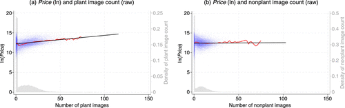
Notes. The model-free results in these images are based on the full sample of 40,294 properties. The scatterplots have jitter added to the x-axes, as the numbers of images are integers. The nonlinear fitted lines used kernel-weighted local polynomial smoothing with the default Epanechnikov kernel and rule-of-thumb optimal bandwidth settings in Stata. Web Appendix H, Figures H1 and H2 depict the zoomed-in version of panels (a) and (b). Web Appendices H.3 and H.4 depict the relationship between property price (log-transformed) and total image count. Of the 40,294 properties, 22.99% had no images and 23.12% had a single image. As seen in the histograms in Web Appendix H, Figure H3, these observations are distributed differently, with large spikes in the distribution, compared with profiles with two or more images. Furthermore, the pattern in prices for these properties also appears different from the rest of the distribution. Prices for properties with two or more images appear to increase linearly with number of plant images. Properties with zero or just one image have higher average prices than most of the rest of the distribution, with their average prices more in line with properties having around 20 images. In the zoomed-in figures (Web Appendix H, Figures H1, H2, and H4), which have these observations removed, the nonparametric and linear trends are virtually identical. We note that the zero-image property profiles were also qualitatively different, with shorter descriptions than those with one or more images (30.5 words versus 42.1 for those with images, t = 49.5, p < 0.001) and were commonly sold without a realtor (94.7% with no realtor versus 16.0% for those with images).
3.4.2. Main Results.
Given the linear relationship between plant image count and log price evident in the model-free results, we adopted an ordinary least squares regression for the main analyses to more formally evaluate their relationship, with nonplant image count as a covariate (Table 2). In Model (1), without any other covariates, the regression coefficient of plant image count is positive (β = 0.0267, standard error (SE) = 0.0022, p < 0.001) and significantly larger than that of nonplant image count (β = −0.0205, SE = 0.0031, p < 0.001; coefficient comparison: p < 0.001). The positive relationship between plant image count and price paid persists after adding property and neighborhood attributes (Model (2)), image and text attributes (Model (3)), zip code fixed effects (Model (4)), and estimated property value from the website (Model (5)) as covariates. In particular, in Model (5), which contains all available covariates, including the zip code fixed effects and website estimated property valuation (claimed to have a median prediction error of 2% compared with the final sale price), plant image count remains positive and significant (Plant Image Count: β = 0.0016, SE = 0.0003, p < 0.001; Nonplant Image Count: β = 0.0007, SE = 0.0004, p > 0.10). Additional analysis shows that across 64 nonredundant models with different covariate combinations, the coefficient for plant image count remains consistently positive and significant, whereas the coefficient for nonplant image count is neither positive nor stable (Web Appendix I.2).
|
Table 2. Main Regression Results
| (1) | (2) | (3) | (4) | (5) | ||||||
|---|---|---|---|---|---|---|---|---|---|---|
| Price(ln) | Price(ln) | Price(ln) | Price(ln) | Price(ln) | ||||||
| Plant Image Count | 0.0267*** | (0.0022) | 0.0183*** | (0.0018) | 0.0154*** | (0.0018) | 0.0054*** | (0.0007) | 0.0016*** | (0.0003) |
| Nonplant Image Count | −0.0205*** | (0.0031) | −0.0225*** | (0.0023) | −0.0062** | (0.0019) | 0.0032** | (0.0010) | 0.0007 | (0.0004) |
| Property attributes (also include indicators of missing lot size, property type, and the house facing direction in Web Appendix I.1) | ||||||||||
| Bedrooms | 0.0165 | (0.0292) | 0.0338 | (0.0247) | 0.0561*** | (0.0160) | −0.0039+ | (0.0023) | ||
| Bathrooms | 0.2331*** | (0.0601) | 0.1931*** | (0.0511) | 0.1157*** | (0.0332) | −0.0010 | (0.0029) | ||
| House Age (ln) | −0.1107*** | (0.0150) | −0.0857*** | (0.0139) | −0.1039*** | (0.0079) | −0.0067*** | (0.0022) | ||
| House Size (ln) | 0.3743*** | (0.0604) | 0.2753*** | (0.0489) | 0.2482*** | (0.0345) | −0.0151*** | (0.0056) | ||
| Lot Size (ln) | 0.0457*** | (0.0129) | 0.0460*** | (0.0109) | 0.0402*** | (0.0065) | 0.0004 | (0.0016) | ||
| NDVI30 | −0.5203*** | (0.0850) | −0.3959*** | (0.0703) | −0.0858* | (0.0382) | 0.0026 | (0.0128) | ||
| NDVI120 | −0.2805*** | (0.0811) | −0.2989*** | (0.0714) | 0.0306 | (0.0396) | −0.0007 | (0.0150) | ||
| NDVI510 | −0.7621*** | (0.1888) | −0.7296*** | (0.1574) | −0.0799 | (0.0679) | −0.0033 | (0.0156) | ||
| Neighborhood attributes | ||||||||||
| Walking Score | 0.0011 | (0.0014) | 0.0017 | (0.0011) | −0.0010+ | (0.0006) | −0.0002 | (0.0001) | ||
| Biking Score | 0.0051** | (0.0017) | 0.0038* | (0.0015) | 0.0014* | (0.0007) | 0.0000 | (0.0001) | ||
| School Rating | 0.1599*** | (0.0368) | 0.1472*** | (0.0315) | 0.0153 | (0.0215) | −0.0054 | (0.0036) | ||
| Image variables (also include six nonplant image content cluster scores in Web Appendix I.1) | ||||||||||
| Exterior Image Count | −0.0149*** | (0.0035) | 0.0000 | (0.0017) | −0.0024** | (0.0009) | ||||
| Photo Quality (std) | 0.0020 | (0.0232) | −0.0144 | (0.0133) | 0.0030 | (0.0046) | ||||
| Property Quality (std) | 0.0221 | (0.0228) | −0.0108 | (0.0103) | 0.0036 | (0.0045) | ||||
| Property Cleanliness (std) | 0.0015 | (0.0143) | 0.0095 | (0.0068) | 0.0063** | (0.0024) | ||||
| Property Attractiveness (std) | 0.0855*** | (0.0238) | 0.0594*** | (0.0113) | −0.0015 | (0.0043) | ||||
| Property Maintenance (std) | 0.0077 | (0.0221) | 0.0303* | (0.0120) | 0.0076* | (0.0036) | ||||
| Property Decoration (std) | 0.0696+ | (0.0373) | 0.0121 | (0.0147) | −0.0039 | (0.0053) | ||||
| Landscaping Quality (std) | 0.0118* | (0.0052) | 0.0034 | (0.0031) | 0.0016 | (0.0012) | ||||
| Occupancy (std) | 0.0112* | (0.0050) | 0.0000 | (0.0025) | −0.0032** | (0.0011) | ||||
| Expensive Furnishing (std) | 0.0279 | (0.0169) | 0.0154* | (0.0074) | 0.0012 | (0.0022) | ||||
| Textual attributes | ||||||||||
| Total Word Count | 0.0026*** | (0.0006) | 0.0024*** | (0.0003) | 0.0005*** | (0.0001) | ||||
| Plant Word Count | 1.5867*** | (0.2911) | 0.0538 | (0.1308) | 0.0286 | (0.0560) | ||||
| Property valuation estimate | ||||||||||
| Web Estimate Price (ln) | 1.0452*** | (0.0179) | ||||||||
| Fixed effects (FEs) | No | No | No | Zip code | Zip code | |||||
| Property/neighborhood attributes | No | Yes | Yes | Yes | Yes | |||||
| Image/text attributes | No | Yes | Yes | Yes | Yes | |||||
| Number of FE groups | NA | NA | NA | 319 | 309 | |||||
| Observations | 31,031 | 25,607 | 25,607 | 25,590 | 22,409 | |||||
| Adjusted R2 | 0.1002 | 0.4831 | 0.5514 | |||||||
| Within-cluster R2 | 0.5378 | 0.8675 | ||||||||
Notes. Values in parentheses are standard errors (std). For certain housing types (e.g., condos), lot size was often missing, so a dummy variable was used to indicate these observations rather than omit them. More discussion of model coefficients is in Web Appendix I.1.
+0.05 < p < 0.10; *0.01 < p < 0.05; **0.001 < p < 0.01; ***p < 0.001.
Thus, the prices paid for homes varied systematically with plant image count (but not with nonplant image count). Selling prices were higher for properties with more (versus fewer) plant images, and the difference persists after including covariates for property and neighborhood characteristics, presentational features such as text or image attributes, and other property or local market condition information available to the real estate platform.
3.5. Alternative Measures for Key Variables
3.5.1. Alternative Plant Imagery Measures.
We checked whether similar results emerged using alternative measures for plant image count (Web Appendix J.1). The results are consistent when substituting the percentage of plant images in each home profile (i.e., plant image count divided by total image count; Model (6)) or the log-transformation of plant and nonplant image counts (Model (7)). We also examined results using plant image counts based on other image classification methods (Models (8)–(12)) and obtained similar results for classifiers with relatively high accuracy, such as Faster R-CNN.
We also ran a model with a dummy variable added to indicate whether a property had any plant images. Consistently, coefficients are positive for the dummy variable and for plant image count, but not for nonplant image count.12 Another analysis, replacing number of nonplant images with total number of images, shows the plant image count coefficient is positive and marginally significant.13
3.5.2. Alternative Market Performance Measures.
In addition to the price paid for a home, we calculated the number of days a property was on market until sold. The real estate website also indicated how many people viewed, liked, and disliked each property profile, and how many physical house tours were scheduled through the website. The results were robust (Table 3), as regards the association between plant images and transaction speed (i.e., reduced days on market; Model (13)), views (Model (14)), likes (Model (15)), dislikes (Model (16)),14 and house tours (Model (17)).15 The results were also consistent using alternative price-based outcomes (Web Appendix J.2), including property sales price in absolute dollars (instead of log-transformed; Model (18)) and price difference (percentage) over the property valuation estimate (Model (19)), listed price (Model (20)), and neighborhood median price (Model (21); see Web Appendix J.2).
|
Table 3. Alternative Market Performance Measures
| Independent variable | (13) Days on Market (ln) | (14) Views | (15) Likes | (16) Dislikes | (17) Tours |
|---|---|---|---|---|---|
| Plant Image Count | −0.0017+ | 1.5832* | 0.1543*** | −0.0096 | 0.0036* |
| (0.0010) | (0.6940) | (0.0338) | (0.0064) | (0.0017) | |
| Nonplant Image Count | 0.0050*** | 0.0195 | −0.1082*** | 0.0215*** | 0.0005 |
| (0.0012) | (0.5158) | (0.0254) | (0.0059) | (0.0013) | |
| Coefficient comparison | p < 0.001 | p = 0.070 | p < 0.001 | p < 0.001 | p = 0.202 |
Notes. For all the models, we used the same set of covariates as in our Model (5). Values in parentheses are standard errors. For Model (13), we note that our sample was selected based on a limited window of transaction dates (June 10 to December 9, 2019), so very old property listings may exhibit survivor biases that attenuated the strength of the main association tested. Perhaps not surprisingly, the conditional association is stronger if restricted to properties sold within a year.
+0.05 < p < 0.10; *0.01 < p < 0.05; ***p < 0.001.
3.5.3. Alternative Property Value Estimates.
The main analysis included the website’s estimated valuation of the property as a covariate. Using instead the last listed price for the home prior to sale (Model (22)) or neighborhood median house price (Model (23)) yielded consistent results (Web Appendix J.3), as did adding the estimated property valuation and last listed price simultaneously (Model (24)).
3.5.4. Alternative Fixed Effects.
Our main analysis used five-digit zip codes for fixed effects. The results are robust to using alternative geographic groupings for fixed effects (Web Appendix J.4), including more coarse-grained three-digit zip codes (Model (25)); geographical cells constructed using one, two, three, or four decimal places of the property coordinates (Models (26)–(29)); or seller’s agent dummies (Model (30)).16
3.6. Exploring Heterogeneity by Image Type and Geographic Market
The main analysis indicated a positive conditional association between plant images and property price paid. As an extension, we explored whether the observed pattern varied by different image characteristics and geographic areas, to document where the association may be more or less pronounced.
We first examined whether the strength of the conditional association between plant image count and property valuation varied by image characteristics. Results show that plant images had a stronger association with prices paid for interior versus exterior images, and for images appearing earlier versus later in a home profile (see Web Appendix J.5, Models (31)–(33)).17 Additional research would be needed to characterize the underlying sources of the heterogeneity.
We then assessed whether the strength of the relationship between plant images and property valuation varied by the prevalence of plant imagery in different geographic areas. We quantified the prevalence of plant imagery using the average percentage of property images that contained plants within each zip code and examined its interaction with our main independent variable, plant image count (Figure 2(b), analysis (34)).18 The results indicate a significant negative interaction between plant image count and geographic prevalence of plant images (β = −0.0076, SE = 0.0017, p < 0.001). A three-way split of the plant image prevalence measure19 shows the association was larger in areas with lower plant image usage (β = 0.0027, SE = 0.0004, p < 0.001; areas with moderate usage: β = 0.0011, SE = 0.0004, p = 0.006; areas with high usage: β = 0.0008, SE = 0.0003, p = 0.017).
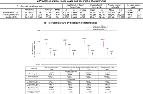
Notes. In panel (a), the three-cell split was based on the 22,409 observations without any missing values in any of the covariates. This is to ensure the coefficients of plant image count are comparable across different buckets. In panel (b), for all the models, we used the same set of covariates as our main Model (5), plus nonplant image count and its interaction with the moderators. Values without parentheses are coefficient estimates, and values with parentheses are standard errors of coefficient estimates. Each analysis in (34)–(37) includes two separate models (one for the interaction analysis, one for the three-cell split analysis). Note that the three-cell split was based on the 22,409 observations without any missing values in any of the covariates. This is to ensure the coefficients of plant image count are more comparable across different buckets. *0.01 < p < 0.05, **0.001 < p < 0.01, ***p < 0.001.
Different neighborhoods vary in prevalence of plant image usage, and our results show that plant images are more strongly associated with property prices in markets where their current use is more limited. What characterizes areas where plant imagery is least versus most common? We found that neighborhoods where plant imagery was least versus most prevalent (Figure 2(a)) were characterized by lower family incomes ($76,167 versus $93,637), lower nearby property values ($253,428 versus $490,831), and lower average image quality for the homes listed for sale (−0.382 versus 0.499). Thus, one reason why plant imagery usage varies across different markets may be related to differences in sellers’ resources. Sellers with greater resource limitations (e.g., time and monetary constraints) may find it more challenging to implement every possible strategy to enhance property presentation, particularly strategies considered relatively low priority, such as adding plant images. Yet our results suggest it is in markets with greater resource constraints that the residual price gap associated with plant imagery is stronger (analyses (35)–(37), Figure 2(b)), an intriguing pattern that deserves closer examination.
4. General Discussion
Despite prior research suggesting extensive benefits from exposure to plants in human living environments, their presence in modern-day, predominantly indoor lifestyles is notably limited, which can negatively impact well-being (Chang and Durante 2022). Some contemporary architectural designers are working to address this issue by incorporating natural elements such as plants and water features into building designs to elevate people’s moods and enhance worker performance (Larsen et al. 1998, Joye et al. 2010, Margolies 2019). Informed by phytophilia theory, which proposes that humans are intrinsically attracted to natural life forms such as plants, we examined whether online home profiles with more images containing plant life have systematically higher transaction prices, after accounting for variation in multiple marketplace factors, including those that have been previously studied, such as property attributes and market expectations. By examining a variable not previously examined in the context of home-buying behavior, plant imagery, our results may generate deeper insights regarding home-buying behavior and spur additional research regarding causal mechanisms and generalizability (Reiss 2011).
We first presented results of a survey among real estate agents suggesting that the use of plants in property presentation is currently a low priority for most house sellers. We then obtained a large data set of sold homes in the United States and assessed the conditional association between plant image count and property sale price. Our results show that properties with more plant images tend to have higher transaction prices as well as higher levels of online engagement and faster transaction speeds. Importantly, the pricing differential exists above and beyond variation in factors such as inherent property and neighborhood attributes, presentation efforts (evident in other aspects of the profile images and texts), and market conditions or expectations. Further analysis showed that the conditional association was stronger when plants appeared in interior versus exterior images, in earlier-appearing images in a profile, and in geographic areas where the use of plant images in home profiles was less common.
The primary limitation of this paper is the observational nature of the data and the descriptive nature of the analysis. Although we cannot explicitly test causal theories or provide prescriptive managerial recommendations, the observed positive association between plant images and property valuation—after accounting for an extensive set of covariates—suggests that plant imagery may carry benefits beyond well-established factors such as inherent property and neighborhood attributes, property presentation efforts, and market conditions or expectations (see Web Appendices E and K.1). Follow-up analyses using double machine learning (Chernozhukov et al. 2017) and coarsened exact matching (Iacus et al. 2012) yielded consistent positive coefficients of plant imagery on property valuation (see Web Appendices K.2 and K.3), but the results cannot be interpreted causally with a high degree of confidence because of the lack of purely exogenous variation in plant imagery. Further research with careful causal design is needed to rigorously test the existence of a causal relationship.
More research is also needed to better understand the heterogeneity observed. Following the idea of using theory to inform descriptive analysis (de Kadt and Grzymala-Busse 2025), we explored heterogeneity with a focus on factors that could relate to attracting home buyers’ attention. Our results suggest that the conditional association between plant images and prices paid is stronger in contexts where plant images are likely to be more salient and thus garner more attention. Plants appearing in interior versus exterior images are likely less expected and may therefore attract more attention through a novelty effect (e.g., Schomaker and Meeter 2012). Similarly, plant images appearing earlier versus later in the images of a home profile may draw more attention because of a primacy effect (e.g., Murdock 1962). Furthermore, we found a stronger association in geographic areas where plant imagery was less prevalent in home profiles and thus possibly less expected, neighborhoods that also tended to face greater resource constraints. Although we do not directly observe mechanisms that comport with phytophilia theory, our findings reveal noteworthy patterns that warrant further investigation.
Future research could also examine whether plant images in other contexts seem to attract more visual attention in accord with phytophilia and evolutionary theory, recognizing the life-supporting role of plant life forms. For example, future research could explore the implications of plant images beyond the residential home selling context. Plant images may be associated with prices and occupancy rates for short-term rentals displayed on websites such as Airbnb or VRBO, where visual presentation plays a central role in decision making. More broadly, as consumers increasingly rely on digital interfaces to evaluate products and services, plant imagery and its associations may become increasingly impactful in technology-mediated environments. It would also be interesting to examine whether other forms of natural elements, such as animals and water features (i.e., biophilia, more broadly) generate similar associations (Terrapin Bright Green 2014, Shin et al. 2023). Although such features may currently be rare in the real estate market context,20 the possibilities in other contexts may provide promising avenues for future research.
1 Centiment is an online data collection platform for targeted audiences and has been widely adopted by marketing researchers (e.g., To and Patrick 2021). We requested 100 real estate agents from Centiment and retained 98 valid responses after attention-check exclusions (Web Appendix B.1). Those agents have an average tenure of 9.74 years, with an average of 8.79 transactions handled per year. Thus, their responses correspond to experience of approximately 8,390 transactions, providing reasonably broad information about practices in the real estate market.
2 Website activity variables (including webpage views, likes, dislikes, and property tours) are no longer provided by the platform.
3 We note that property profiles with no images or just one image were distributed somewhat differently, with the patterns in prices for these properties appearing to differ from the rest of the distribution (Figure 1). We retained property profiles with one or more images for the main analysis. The results, however, are consistent when also including property profiles with zero images, or when including only property profiles with two or more images.
4 Some may be concerned that property profiles may change after being sold. Theoretically, changing property profiles (e.g., removing house images) is mostly out of privacy concerns from the owners, which should be orthogonal to the property sales process. To further address this problem, we checked the house profiles again six months after the scraping. Only 2,335 out of 31,031 houses (7.52%) were found to have image changes (and 557 were because of a relisting). The analysis results are consistent after removing these houses.
5 We adopted the zero-shot approach rather than fine-tuning as it is among the most common and efficient ways to implement LMMs (see Web Appendix F.1). Notably, zero-shot classification with the LMMs achieved near-ceiling accuracy (approximately 95%) in our context, leaving limited scope for further gains from fine-tuning, consistent with the findings from Ye et al. (2025).
6 The image classification prompt used was, “Please classify the image based on whether it contains plants or not.” The object detection prompt used was, “Please detect all plant objects in the image and classify the image based on whether it contains plants or not.” We defined a structured output schema to standardize model responses, which included a binary plant classification and a probability score of the classification for image classification tasks, and plant locations in bounding-box format for object detection tasks.
7 In total, we labeled 5,141 images: 4,000 of the images were used for model training, 500 for model validation, and 641 for model evaluation. Only the CNN and Faster R-CNN models required model training and validation. In addition to a binary label for each image, human coders also drew bounding boxes (i.e., rectangles) around each identified instance of plant life with VGG Image Annotator (Dutta and Zisserman 2019) in order to train object-detection models, for example, Faster R-CNN.
8 We did not use similar LMMs for evaluating image attributes or image content more commonly related to property values because these models were developed after the property transactions occurred and thus may have encoded price information in their knowledge bases (Lee 2025). By contrast, plant image classification is a more objective task that is likely less influenced by market information and can therefore be used more safely for estimation. Nevertheless, as a check, we used GPT-5-mini to evaluate image attributes and found its prediction performance comparable to that of the trained CNN models. The results remained consistent when image attributes generated by GPT-5 mini were included as covariates (Plant Image Count: β = 0.0009, SE = 0.0003, p = 0.003).
9 The 3,649 image labels were classified by two independent human coders (98.96% agreement rate).
10 Although the alternative property valuation estimation measures reflect additional information available to property owners and help account for local market and the property characteristics, the list price itself may be endogenous to the home selling process, and the neighborhood median sales price is superseded by the other two valuation measures along with the zip code indicator. Hence, we used website’s estimated home value as a conditioning factor in the main model (Model (5)), and used the other two for robustness checks.
11 In the full sample of 40,294 properties, each had 14 images on average, of which 60.01% (about 9 images) depicted plants. The correlation with log price was stronger for the number of plant images (r = 0.269, p < 0.001) than for the total number of images (r = 0.195, p < 0.001).
12 The coefficient for the dummy variable is β = 0.0216 (SE = 0.0114, p = 0.059). The coefficient for Plant Image Count is β = 0.0016 (SE = 0.0003, p < 0.001). The coefficient for Nonplant Image Count is β = 0.0006 (SE = 0.0004, p = 0.131; coefficient comparison: p = 0.059).
13 The coefficient for Plant Image Count is β = 0.0009 (SE = 0.0005, p = 0.063). The marginal significance is likely due to a high correlation between plant image count and total image count. In this specification, the coefficient for the plant image count also has a different interpretation: it captures the impact of replacing a nonplant image with a plant image while holding the total number of images constant. The positive coefficient indicates that such a substitution is still associated with a more favorable outcome. It also suggests that the documented association in our main analysis is tied to plant imagery specifically rather than the overall quantity of visual information provided in the listing.
14 The coefficient of plant images on the number of dislikes is only marginal (p = 0.132), possibly because house hunters tend to focus on building their consideration set rather than their cross-out set, unless a property is strongly aversive in light of their preferences.
15 Although the association between plant images and tours was small, it may indicate that more users scheduled showings through their own realtors (which we do not observe) before becoming potential buyers (the same images are typically shown across all other major real estate websites).
16 In our data set, only 26,072 out of 31,031 properties have realtor information. In total, we identified 6,871 unique realtors; each realtor was associated with 34 properties on average, and 3,790 realtors handled only one property. Because this variable is noisy with many missing values, and including it as fixed effects would consume many degrees of freedom, we did not include it in our main analysis.
17 Model (31) does not include nonplant image count, but includes both interior and exterior image counts. A joint test of the regression estimates for interior and exterior plant image counts is significant.
18 For each model, we included both and as the predictors (i and j represent property i from zipcode j). We also included the full set of covariates from our preferred Model (5), as well as and .
19 We categorized each moderator into three groups and used to denote the cell (bottom, middle, or top third of the population) to which property i (from zip code j) belongs. We then estimated the plant imagery–price association across the three cells with as the predictor. Each model included the full set of covariates from our preferred Model (5) and .
20 Using a random sample of 5,141 images (the same subset used to train and evaluate the plant image classification models), we found that 68.49% of the sampled images contained plants, compared with 0.14% containing animals (such as birds, deer, horses, cats, or dogs), 0.21% containing human presence, 0.95% containing mountains, and 3.37% containing water features (such as lakes, oceans, or pools).
References
Attom (2020) Average U.S. home seller profits hit $65,500 in 2019, another new high. Retrieved December 6, https://www.attomdata.com/news/market-trends/home-sales-prices/attom-data-solutions-year-end-2019-u-s-home-sales-report/.Google Scholar- (2003) Latent Dirichlet allocation. J. Machine Learn. Res. 3(January):993–1022.Google Scholar
- (2012) The impact of in-store greenery on customers. Psych. Marketing 29(11):807–821.Crossref, Google Scholar
- (2008) Information and real estate transactions: The effects of pictures and virtual tours on home sales. Working paper, Department of Economics, The George Washington University, Washington, DC.Google Scholar
- (2022) Why consumers have everything but happiness: An evolutionary mismatch perspective. Current Opinion Psych. 46:101347.Crossref, Google Scholar
- (2017) Double/debiased/Neyman machine learning of treatment effects. Amer. Econom. Rev. 107(5):261–265.Crossref, Google Scholar
- (2025) Good description. SocArXiv preprint, submitted May 22, https://doi.org/10.31235/osf.io/e74a9_v1.Google Scholar
- (2019) The VIA annotation software for images, audio and video. Amsaleg L, Huet B, Larson M, Gravier G, Hung H, Ngo CW, Ooi WT, eds. Proc. 27th ACM Internat. Conf. Multimedia (Association for Computing Machinery, New York), 2276–2279.Google Scholar
- (2021) Visual elicitation of brand perception. J. Marketing 85(4):44–66.Crossref, Google Scholar
- (2024) Home-selling checklist: 12 things to do before selling your house. Retrieved June 19, https://www.realtor.com/advice/sell/home-selling-checklist-things-to-do-before-selling/.Google Scholar
Google DeepMind (2025) Gemini 2.5 Flash. Accessed August 17, 2025, https://deepmind.google/models/gemini/flash/.Google Scholar- (2012) Causal inference without balance checking: Coarsened exact matching. Political Anal. 20(1):1–24.Crossref, Google Scholar
- (2011) Is love for green in our genes? A critical analysis of evolutionary assumptions in restorative environments research. Urban Forestry Urban Greening 10(4):261–268.Crossref, Google Scholar
- (2010) The effects of urban retail greenery on consumer experience: Reviewing the evidence from a restorative perspective. Urban Forestry Urban Greening 9(1):57–64.Crossref, Google Scholar
- (1998) Plants in the workplace: The effects of plant density on productivity, attitudes, and perceptions. Environ. Behav. 30(3):261–281.Crossref, Google Scholar
- (2025) Generative brand choice. PhD thesis, University of Chicago, Chicago.Google Scholar
- (2020) Is a picture worth a thousand words? An empirical study of image content and social media engagement. J. Marketing Res. 57(1):1–19.Crossref, Google Scholar
- (2020) Visual listening in: Extracting brand image portrayed on social media. Marketing Sci. 39(4):669–686.Link, Google Scholar
- (2019) Listing agent signals: Does a picture paint a thousand words? J. Real Estate Finance Econom. 59(4):617–648.Crossref, Google Scholar
Madison Trust (2024) How much an average home has cost in the United States over time. Retrieved December 6, https://www.madisontrust.com/information-center/visualizations/how-much-an-average-home-has-cost-in-the-united-states-over-time/.Google Scholar- (2019) Making a day at the office like a walk in the park. Accessed December 1, 2025, https://pacificworkplaces.com/blog/making-a-day-at-the-office-like-a-walk-in-the-park/.Google Scholar
- (2019) Principles of Economics (Ludwig von Mises Institute, Auburn, AL).Google Scholar
- (2023)
Scaling open-vocabulary object detection . Oh A, Naumann T, Globerson A, Saenko K, Hardt M, Levine S, eds. Advances in Neural Information Processing Systems, vol. 36 (Curran Associates, Red Hook, NY), 72983–73007.Crossref, Google Scholar - (2022)
Simple open-vocabulary object detection . Avidan S, Brostow G, Cissé M, Farinella GM, Hassner T, eds. Computer Vision—ECCV 2022 (Springer, Cham, Switzerland), 728–755.Crossref, Google Scholar - (1962) The serial position effect of free recall. J. Experiment. Psych. 64(5):482–488.Crossref, Google Scholar
National Association of Realtors (2021) Home buyers and sellers generational trends report. Accessed January 15, 2024, https://www.nar.realtor/sites/default/files/documents/2021-home-buyers-and-sellers-generational-trends-03-16-2021.pdf.Google ScholarOpenAI (2025) Introducing GPT-5. Accessed August 17, 2025, https://openai.com/index/introducing-gpt-5/.Google Scholar- (2021) Learning transferable visual models from natural language supervision. Marina M, Zhang T, eds. Proc. 38th Internat. Conf. Machine Learn. Proceedings of Machine Learning Research, vol. 139 (PMLR, New York), 8748–8763.Google Scholar
- (2011) Descriptive, structural, and experimental empirical methods in marketing research. Marketing Sci. 30(6):950–964.Link, Google Scholar
- (2017) Faster R-CNN: Towards real-time object detection with region proposal networks. IEEE Trans. Pattern Anal. Machine Intelligence 39(6):1137–1149.Crossref, Google Scholar
- (2011) Validation of the normalized difference vegetation index as a measure of neighborhood greenness. Ann. Epidemiology 21(12):946–952.Crossref, Google Scholar
- (2012) Novelty enhances visual perception. PLoS One 7(12):e50599.Crossref, Google Scholar
- (2023) Connecting nature with luxury service. Psych. Marketing 40(2):300–316.Crossref, Google Scholar
- (2015) Very deep convolutional networks for large-scale image recognition. Bengio Y, LeCun Y, eds. Proc. Third Internat. Conf. Learn. Representations (Computational and Biological Learning Society, San Diego, CA), 1–14.Google Scholar
- (2005) The composition of hedonic pricing models. J. Real Estate Literature 13(1):1–44. Crossref, Google Scholar
Terrapin Bright Green (2014) The Economics of Biophilia (Terrapin Bright Green, LLC, New York).Google Scholar- (2017) Phytophilia and service atmospherics: The effect of indoor plants on consumers. Environ. Behav. 49(7):814–844.Crossref, Google Scholar
- (2021) How the eyes connect to the heart: The influence of eye gaze direction on advertising effectiveness. J. Consumer Res. 48(1):123–146.Crossref, Google Scholar
- (1984) Biophilia (Harvard University Press, Cambridge, MA).Crossref, Google Scholar
- (2025) LOLA: LLM-assisted online learning algorithm for content experiments. Marketing Sci. 44(5):995–1016.Abstract, Google Scholar
Yuqian Chang is an assistant professor in marketing at Ivey Business School, Western University. Her current work focuses on unstructured data for marketing insights, and emerging technology applications in business. Yuqian obtained her PhD in marketing from Rutgers University.
Nathan Fong is an associate professor in marketing at the School of Business, Rutgers University Camden. His research evaluates marketing mix effects in digital marketing settings. He received his BS from Stanford University and his PhD from MIT.
Ning Ye is an associate professor of marketing at Stockton University. Her research examines consumer behavior, with a particular focus on health, food, social media, and emerging technologies. She earned an MS in marketing from Johns Hopkins University and a PhD in marketing from Temple University.
Maureen (Mimi) Morrin is a professor emeritus in marketing at Rutgers University Camden. Her research focuses on sensory processing, investigating the effects of scent, touch, vision, taste, and sound on the consumer decision-making process. She has served as coeditor at the Journal of Marketing Research and an area editor at the Journal of Consumer Psychology. She received her BSFS from Georgetown University, MBA from Thunderbird, and PhD from New York University.