


Algorithm Supported Induction for Building Theory: How Can We Use Prediction Models to Theorize?
Abstract
Across many fields of social science, machine learning (ML) algorithms are rapidly advancing research as tools to support traditional hypothesis testing research (e.g., through data reduction and automation of data coding or for improving matching on observable features of a phenomenon or constructing instrumental variables). In this paper, we argue that researchers are yet to recognize the value of ML techniques for theory building from data. This may be in part because of scholars’ inherent distaste for predictions without explanations that ML algorithms are known to produce. However, precisely because of this property, we argue that ML techniques can be very useful in theory construction during a key step of inductive theorizing—pattern detection. ML can facilitate algorithm supported induction, yielding conclusions about patterns in data that are likely to be robustly replicable by other analysts and in other samples from the same population. These patterns can then be used as inputs to abductive reasoning for building or developing theories that explain them. We propose that algorithm-supported induction is valuable for researchers interested in using quantitative data to both develop and test theories in a transparent and reproducible manner, and we illustrate our arguments using simulations.
Introduction
Building theory from specific data involves proposing general processes, features, and relationships between means and ends around a particular phenomenon. Such theory building occupies a central role in the organizational sciences, as it does in any science that gives the explanation of phenomena at least as much importance as the testing of deductively derived implications from axioms (Glaser and Strauss 1967, Lave and March 1993, Deetz 1996, Walsh et al. 2015, Bamberger 2018). However, explicit theory building from data in management and organization research has traditionally been reserved for researchers working with small numbers of cases rather than for those working with large N data. Moreover, the norms for presenting quantitative papers often involve proposing theoretically derived hypotheses and then testing them, and this may sometimes obscure, de-emphasize, and delegitimize inductive reasoning, even if it plays an important role in generating the results (Gelman and Loken 2014, Goldfarb and King 2016).
In this paper, we argue that machine learning (ML) represents a useful new methodology to enable theory building from data for organization scholars working with large samples of data. ML can facilitate algorithm-supported induction, yielding interpretable conclusions about patterns in data that are likely to be robustly replicable by other analysts and in other samples from the same population. This can be accomplished, as we demonstrate, with well-established ML algorithms that are neither new to the world, nor new to the field of ML. What we consider new, and more importantly, valuable to the field of organization science, is our approach to using ML for the specific purpose of algorithm supported induction as a step in the process of building theory from data.
To fully understand the role of algorithm-supported induction in theory building, it is useful to first review different forms of reasoning. Deduction of theoretical implications from known axioms is at the heart of hypothesis testing research (Popper 1959). In contrast, induction of a pattern from the data and abduction of an explanation for the pattern are core to the theory-building process (Peirce 1878, Bamberger 2018, Behfar and Okhuysen 2018). Although ML plays a key role in induction by revealing robust patterns, it does not (yet) offer a solution to conducting abduction. As of today, what Henry Mintzberg stated in 1979 still holds true: “The data do not generate the theory—only researchers do that—any more than the theory can be proved true in terms of the data” (Mintzberg 1979).
What algorithm-supported induction indeed offers is the detection of complex but interpretable patterns in data in a robust and replicable manner. By interpretable, we mean ML algorithms can be tuned to detect complexity in patterns that would not always be intuitive for humans to identify but intuitive enough to understand once found. By robust and replicable, we mean that ML algorithms (a) incorporate procedures that avoid overfitting (i.e., avoid producing results that are highly idiosyncratic to the observed sample) and (b) applies procedures—including inevitable judgement calls—that are codifiable, thereby enabling replication. However, other fundamental steps in the theory-building process that precede and follow the generation of these robust patterns or stylized facts (Helfat 2007), such as conceptualization (defining the constructs of interest), measurement (selecting or developing measures for the constructs), and explanation (theorizing about the relationships among the observed patterns), remain largely human prerogatives.
To be sure, the applications of ML in management and organization studies are broader than algorithm-supported induction (Tonidandel et al. 2018, von Krogh 2018, Shrestha et al. 2019). For instance, by using a small amount of hand-coded data as the training set, algorithms can learn the patterns implicit in this coding and predict the coding for a much larger data set (Medlock and Briscoe 2007; Crowston et al. 2010, 2012; Yan et al. 2014; Christensen et al. 2017). ML-based data text analytic approaches such as Latent Dirichlet Allocation (LDA) are becoming popular to discover themes and trends in a large collection of documents (Blei 2012, Bao and Datta 2014, Puranam et al. 2017, Huang et al. 2018, Hannigan et al. 2019). In economics, researchers have introduced ML techniques in conjunction with instrumental variable analysis (which requires prediction accuracy in stage-one models) to improve causal inferences (Belloni et al. 2013). ML techniques can also be used as an alternative to propensity score matching (Varian 2016). Another application in economics pertains to estimating heterogeneity in causal effects (Athey and Imbens 2016). Mullainathan and Spiess (2017) provide an overview of ML applications in economics (Varian 2014, Kleinberg et al. 2015).
Although the applications noted previously are all worthy of consideration for more widespread use in our field, our perspective focuses on the application of ML techniques as a tool for building theory from data, which plays a central and perhaps unique role in management and organizations research (Leonard-Barton 1990, March et al. 1991, Sutton 1997, Eastman and Bailey 1998, Burton and Obel 2011).
In the rest of this paper, we propose and illustrate a procedure to conduct algorithm-supported induction. First, we provide a concise and accessible introduction to the core logic of ML principles, with details available in Appendix A for the interested reader. Second, we offer a perspective on how management and organization researchers can conduct algorithm-supported induction by using ML’s core analytical property—detecting robust and replicable patterns of tunable complexity (i.e., researchers can adjust the degree of acceptable complexity in the patterns uncovered). Third, we illustrate (with a simple example using simulated data) how a researcher can apply the technique to build and test theory in the same data, without running the risks of overfitting and low replicability of results. Our illustration unveils the tradeoff between comprehensibility and predictive accuracy that theory building from data inevitably entails and suggests how one might approach this tradeoff in the research process.
What Do ML Algorithms Do?
In this section, we give a brief overview of the basic features of ML methods. Readers familiar with the techniques can skip directly to the next section that describes how we propose to apply it to theory building. ML is a subdomain within the field of artificial intelligence (AI). It endows computers with “the ability to learn without being explicitly programmed” (Samuel 1959, p. 120). Mitchell (1997, p. 2) provided the classic statement about the components of a learning problem that ML algorithms can tackle: “A computer program is said to learn [effectively; author’s note] from experience E with respect to some class of tasks T and performance measure P if its performance at tasks in T, as measured by P, improves with experience E.” Suppose that task T is that we want to predict the profits of a firm in the current year and future years. We want to do this based on the data from past years’ experience (E). Experience may comprise data on past profits with a set of predictors such as price and sales changes, chief executive officer (CEO) characteristics, organization design, planned expenditures, demand trends, liquidity position, or any of the factors that researchers believe are associated with firm profitability. The performance of the algorithm (P) is considered satisfactory if it can predict a firm’s profits accurately. Hence, with increasing data from experience, the algorithm should behave in such a way that the difference between the actual and predicted profit is minimized.
Broadly, two classes of algorithms have been developed to tackle such problems involving learning from existing data: supervised and unsupervised learning.1 Supervised learning involves learning what associates with a given outcome. In the terms of the learning problem discussed above, the goal of a supervised learning algorithm is to make good predictions about future profits (future Ys) based on knowing only the future Xs. This is accomplished by fitting a model that does a good job of predicting past Ys based on past Xs and then assuming that the same relationship between Xs and Ys will hold in the future. The fitted model captures this insight in the form of a function that maps predictors to profit.
Of course, we could also obtain such a prediction using familiar ordinary least squares (OLS) regression. Through techniques such as stepwise regression, we can also find the best fitting model (i.e., linear weighted combination of Xs) that predicts Y in the past data and then use this model to make predictions about future Ys based on future Xs. However, ML algorithms combine two features in a useful manner to improve on such techniques: tunable complexity of functional form and improved protection against overfitting (Abu-Mostafa et al. 2012).
First, with ML, complex functional forms (e.g., higher-order and interaction terms among the Xs) can be incorporated without necessarily having to be specified in detail in advance. For instance, random forest models allow for fitting a hierarchical interaction structure, and neural networks can help fit arbitrarily complex polynomials (Breiman 2001, LeCun et al. 2015). The resulting models can achieve higher levels of fit in the data, which hopefully leads to better predictions in the future. This complexity in functional form may also make the models harder to interpret. For this reason, a feature of ML algorithms that may prove extremely useful to the inductive and abductive theorist is that we can, with many model families, tune the extent of complexity we are willing to tolerate: second-order but not third-order polynomials, or 4 versus 40 coefficients, for instance. We can start with a model family that can accommodate considerable complexity but then use the data to fit a model that can be of considerably lower actual level of complexity. This tuning is done through model hyperparameters, and we can tune these both algorithmically (for maximizing predictive accuracy given the model family) and manually (for interpretability). (Technical details can be found in Appendix A).
Second, ML algorithms enlarge the set of procedures that we commonly use in traditional statistical models to guard against overfitting. For example, if we were to build a well-fitting OLS model by selectively adding or dropping variables to find significant effects, we would run two related risks of overfitting: (a) excessive model complexity—the realized R2 may be high simply because we have too many parameters in the model, and the model must be penalized for this to enable comparison with other models; and (b) excessive sample dependence—including cherry-picked variables can produce a model that may fit the particular sample of data but may not be generalized beyond the data at hand. Both pose fundamental challenges to the validity of the results for understanding future samples. ML algorithms combine an automated model building process (which allows us to find acceptably complex functional forms) with sophisticated procedures for mitigating both types of overfitting. The details of these procedures, namely regularization and cross-validation, can also be found in Appendix A.
Unsupervised learning algorithms, as the name suggests, operate in the absence of a supervisor variable. The data (E) lack any specific target outputs (i.e., Y) associated with each input. These algorithms are generally tasked with detecting patterns of association between groups of X variables, without any particular variable being selected as the dependent variable. Statistical clustering is a canonical example of unsupervised learning with which most management scholars are already familiar. Its purpose is to partition cases into subsets such that similar cases are in the same cluster and dissimilar cases are in different clusters. In our profit prediction example, unsupervised learning can help users find a cluster of firms that are similar to one another on observed dimensions such as CEO attributes, demand trends, and profitability. Strategic group analysis (Harrigan 1985) is a well-established methodology in strategy where studies have frequently used statistical cluster analysis. Unsupervised ML techniques use the same basic logic but provide more flexibility in terms of choosing different types of algorithms to perform the clustering, followed again by procedures such as regularization and cross-validation to prevent overfitting. The relevant algorithms include K-means, hierarchical, and spectral clustering, all of which largely share a similar intuition. LDA is a powerful suite of unsupervised learning algorithms that detect clusters of topics in a corpus of text. It is already extensively in use by organizations researchers (Hannigan et al. 2018).
It is important to highlight that often the same models can be used either for traditional hypothesis testing (i.e., inferential statistics) or for ML (i.e., statistical learning). For instance, OLS regression (Bishop 2006, p. 140; Robert 2014, p. 217; Shalev-Shwartz and Ben-David 2014, p. 123) and logistic regression (Bishop 2006, p. 205; Robert 2014, p. 245; Shalev-Shwartz and Ben-David 2014, p. 126) can both be used for supervised ML, and principal component analysis is a standard tool for unsupervised ML (as well as a standard tool in conventional multivariate analysis) (Shalev-Shwartz and Ben-David 2014, p. 324). The difference between ML and traditional inferential statistics is not rooted in the models per se (although ML in general has many additional model families that allow for more nonlinearity), but in (1) objectives for using them and (2) their accompanying assumptions.
First, inferential statistics are primarily used for testing hypotheses derived from a priori theories, whereas statistical learning, as the name suggests, is used to learn the patterns in data. Second, in inferential statistics it is necessary to assume the distribution of partial density functions of data in order to draw conclusions about statistical significance and potential confidence intervals. In ML, that assumption is not necessary because the goal is predictive accuracy and not inference (Bzdok 2017).
In sum, it is crude but accurate to think of ML algorithms (both supervised and unsupervised) as enabling prediction through searching in data for complex, robust, and replicable associations—complex associations between variables that are unlikely to be the result of sample idiosyncrasy and can be rediscovered by anybody using the same procedures. The complexity and robustness in associations produced by ML algorithms result from procedures that allow (tunably) complex models to fit the data (reducing bias in prediction) while also mitigating against overfitting (reducing variance in predictions). A fundamental theorem in machine learning research pertains to this tradeoff between bias and variance (see Appendix A), and most ML algorithms explicitly aim to optimize this tradeoff to maximize predictive accuracy given the constraints inherent in a model family.2 Replicability, on the other hand, is a property of the algorithmic nature of the process.
However, before we explain how ML techniques can aid theory building from data, three caveats must be stated. First, ML methods are not by themselves a substitute for randomization to obtain causal inference. All ML methods are associative, although they can play an important role in enabling causal inference under the assumption that there are no omitted variables that can create spurious relationships (Pearl 2000; Davis and Heller 2017, p. 548; Athey et al. 2019, p. 20). Second, underlying all ML methods is an assumption that the future can be predicted from the past (more technically, an assumption that probability distributions for the relevant variables remain stationary over time). Hence, current ML algorithms work best for relatively stable phenomena (e.g., in the example above, firm membership in strategic groups and within-group collective behavior is likely to be stable over some extended period of time given strategic and organizational inertia, strategic group mobility barriers, etc.) Third, ML techniques are not geared toward testing an explanation through inferences about the relationships between variables; instead, they focus primarily on prediction (y hat not beta, to use econometric terminology, as noted by Mullainathan and Spiess 2017).
How ML Can Aid Theorizing from Data
We propose that ML algorithms can play a powerful role in aiding theorizing from data by providing a key ingredient necessary for it—robust patterns in data. Such patterns form the basis for prediction by these algorithms, but at the same time they can also be treated as a robust stylized fact to be explained through theorizing and in turn replicated in additional data (Helfat 2007). This stylized fact can then become the target of explanation by the theorist. We see three advantages to separating the process of theorizing into pattern detection (primarily algorithmic and aided by ML techniques) and pattern explanation (primarily nonalgorithmic and driven by human researchers).
First, algorithmic pattern detection has high intersubject reliability. An algorithm used by different individuals will still yield (highly) similar results. This does not preclude the need to make judgement calls in applying algorithms (e.g., which learning algorithm to apply to the data to obtain high predictive accuracy while keeping results interpretable). Our point, however, is that these can be made in a structured, traceable manner, which enables replicability and assessment of robustness. Even for algorithms that involve random components, reproducibility of results can be guaranteed when one keeps track of underlying random seeds used to start off a random number generator. Furthermore, in conventional inductive research methods, where pattern detection and interpretation may occur simultaneously, it is recognized that researchers’ confirmatory biases and motivated information processing could potentially lead to false positives or false negatives (e.g., seeing patterns that are explainable in an intuitive or interesting manner but not seeing others that are less intuitive).3 Analytically separating these steps and performing the first algorithmically enhances replicability. This is not necessarily an advantage if the goal is to enhance creative variation of interpretation and gain novel insights, but it is an advantage if we seek to enhance the reproducibility of an inductive inference.
Second, pattern detection through ML algorithms need not have default human comprehension constraints. For instance, we doubt that any management theorist would hold an entrenched view about the key relationships in their models being linear, although linear models tend to be our workhorse for summarizing multivariate relationships. The advantage of assuming linearity is interpretability, and we willingly give up (some) predictive accuracy for it. If interpretability were not important, we would simply optimize predictive accuracy, but if the goal is to build human comprehensible explanations (i.e., theory), interpretability is key. An advantage with ML algorithms is that the researcher can tune the complexity of patterns the algorithms will detect, depending on his or her goals, taking a more nuanced approach to the tradeoff between predictive accuracy and interpretability rather than just maximizing one or the other. Suppose that a researcher’s appetite for complexity is limited to no more than the second-order interactions with concave functions and no more than a few coefficients overall, ML algorithms can then be set up to find a predictive model that is least likely to over or underfit the data subject to these constraints.
Third, ML algorithms offer protection against results that are highly idiosyncratic to a sample (overfitting). If the central problem in deductive theory testing is spuriousness (i.e., omitted variables that provide alternative explanations), the central problem in theorizing from data are overfitting (i.e., patterns that do not generalize to other samples). However, it has not been given nearly as much attention as the problem of spuriousness, for which we have available a suite of statistical techniques (e.g., instrumental variables, matching, regression discontinuity designs, and ideally, of course, randomization). ML algorithms come equipped with procedures such as regularization and cross-validation that help mitigate the overfitting problem and aid the researcher in detecting (if they exist) reliable associations that replicate across subsamples of data. This is an advantage if we wish to build generalizable theory that can predict out of sample from our inductive and abductive efforts. It is irrelevant if we only seek to generalize to theory based on one or a few cases (Yin 2009). However, to the extent researchers want their theories to be applicable in other samples, overfitting their original sample is always an important concern.
In sum, our central argument is that ML algorithms selected with interpretability in mind can play a useful role in generating robust patterns that are an input to theory building from data. We develop this argument in detail by discussing the elements of algorithm supported induction to aid theory building.
A Procedure to Conduct Algorithm-Supported Induction
We propose a procedure for algorithm-supported induction in Table 1. This procedure we propose can be helpful in creating theory from data by establishing robust stylized facts as an input to abductive theory creation and creating a separate hold out sample for testing the theory without running the risk of overfitting. Although our current description relies on ML algorithms4 in stage 2, the entire procedure itself can be thought of as a meta-algorithm for inductive theorizing and testing of the constructed theory with large sample data.
|

Table 1. Algorithm-Supported Induction: Overview
| Stage | Actions | Procedural details | Human judgment involved |
|---|---|---|---|
| Stage 1: Splitting the sample | Splitting the sample into two random subsamples | Depending on the size of the data set, randomly subsample data into two parts (e.g., 50/50, 80/20) and label them as sample I (for inductive analysis) and sample II (for hypothesis testing) | Choice of initial variables may be shaped by availability, initial unsystematic observation, weak theoretical conjectures. |
| Stage 2: Detection of robust and interpretable patterns | 2.1. Identifying robust associations within sample I | Given a set of feature X, apply a feature selection algorithm to obtain a smaller set of relatively important features without imposing an interpretability constraint on functional form. Use cross validation for hyperparameter tuning. | Selection of algorithms |
| 2.2. Identifying interpretable and robust associations within sample I | Decide on the maximum tolerable level of complexity in terms of interpretability to define a new set of features P. Apply a more interpretable feature selection algorithm on P to obtain a smaller set of relatively important features Use cross-validation for hyperparameter tuning and subsample (or bootstrap sample) replication for robust feature selection. | Selection of acceptable degree of complexity to aid interpretation induction supported by algorithms: identification of a robust and interpretable pattern: that is, function linking variables of interest, in the data (stylized facts) | |
| Stage 3: Theory formulation | Construct a theory that explains p (primary hypotheses) and derive corollary hypotheses from this theory | Thinking and theorizing | Abductive thinking: what is a theory, that if true, would account for the patterns derived from stage 2.2? Deductive thinking: What are additional testable implications (hypotheses) of such a theory? |
| Stage 4: Theory testing | Test implications of theory formulated in stage 3 | Test the primary and corollary hypotheses in the hold-out (sample II) to confirm both out of sample and out of pattern predictions | Operationalization of hypotheses; evaluating statistical and economic significance of results |
In stage 1, we split the data randomly into samples I and II. Sample I is reserved for pattern detection, and Sample II is the hold-out sample (Goldfarb and King 2016). We use sample I to search for interpretable robust patterns in the data (Locke 2015), which we explain by constructing a theory and use sample II to test the hypotheses derived from the theory. If the original full sample is representative of the population, a random subsample of it also will be representative of the population. If the original sample is not representative of the population, any inference procedure (including conventional hypothesis testing) is futile anyway. The procedure we advocate does not therefore raises any new constraints.
Beyond the idea of a hold-out sample, however, algorithm-supported induction also adds some key ingredients. The search for patterns when aided by ML can allow for tunable complexity. Our goal is finding robust and comprehensible associations, not necessarily maximizing predictive accuracy (which is the case in more typical ML applications). This is why stage 2 has two parts. In effect we do two-stage feature selection to generate interpretable patterns. In stage 2.1, we find important features in a predictive model. Using an algorithm that can capture complex functional form without the need to be interpretable, a small set of most important features that contribute the most to predictive accuracy is identified. From the identified features, in stage 2.2, we construct a predictive model from a model family that is relatively easy to interpret.
For instance, in a supervised learning exercise, we might use a random forest or a neural network model in stage 2.1 to give us the most important features that predict an outcome of interest. In stage 2.2, a low degree polynomial (with the degree decided by the researcher, typically of degree 1, linear, or degree 2, two-way interactions and quadratics) constructed from the important variables identified in stage 2.1 can then be put through a second stage of feature selection using an easy to interpret model, such as LASSO (least absolute shrinkage and selection operator) or RIDGE regression.5 Critically, in both stages 2.1 and 2.2, we use cross-validation for hyperparameter tuning (a process that produces a model that is optimized for predictive accuracy given constraints of the model family). In addition, in stage 2.2, we conduct subsample (or bootstrap sample) replication to ensure that the patterns (i.e., the specific associations between variables) we end with are robust to sampling error.
This two-stage feature selection process aims to balance predictive accuracy of the stylized patterns obtained in the data, with interpretability, which is critical if these patterns are to be useful as inputs to abductive theorizing. As shown in Figure 1 (left), the optimal complexity of a ML model estimated from the data and to be used for prediction will optimize the bias-variance tradeoff subject to the constraints of the model family. A particular model (i.e., the set of nonzero coefficients in an OLS model if the model family used is OLS) achieves the lowest distance between training set error (shown by small dotted lines) and test set error (shown by longer dotted lines), indicating that the model does not either overfit or underfit the data (Bishop 2006, Abu-Mostafa et al. 2012, Alpaydin 2014). Such an optimized model is not necessarily a perfect representation of the underlying data generation process (because we have assumed a model family, OLS with its linearity in parameters assumption, which may or may not correspond to the underlying data generation process of a phenomenon) but rather one that fits the data as best as possible (i.e., neither over- nor underfits) given the constraints of the model family (e.g., the general functional form of an OLS regression in this case).

In organization science, validity may be conceptualized in terms of correspondence to the underlying data generation process (Shadish et al. 2002). A valid model in this sense is one that not only optimizes predictive accuracy (optimizes error in training and test data) for a given model family but also has the lowest absolute values of prediction error possible. Minimizing prediction error through optimizing the bias-variance tradeoff is therefore a precondition to having the lowest absolute prediction error. This implies that if the prediction error is not even optimized within a model family, then we know it definitely cannot be at its global minimum (i.e., the model cannot be a valid model).
This leads to the critical interpretability/prediction error tradeoff: as we impose tighter restrictions on interpretability, prediction accuracy will necessarily decline. For our purposes, we think of interpretability simply as researcher’s ability to understand and explain the results of a model to each other.6 To illustrate why interpretability may not come for free, we can superimpose a difficulty of interpretation function over the bias-variance tradeoff reported in Figure 1 (right). Assuming that the interpretation difficulty function is increasing more rapidly in complexity than the variance in predictions it follows that (a) the best interpretable model likely underfits the data—it is therefore likely to have lower prediction accuracy than a model that optimizes the bias-variance tradeoff—and (b) models optimizing the bias-variance tradeoff may have high interpretation difficulty.
It is therefore inevitable that as we select model families that allow for greater complexity of functional form, we will at some point also sacrifice interpretability. As long as the world is complex (i.e., the underlying data generating processes can be of arbitrary complexity) but humans are boundedly rational (i.e., limited in their ability to comprehend and explain complexity to each other), researchers will have to make their own tradeoffs between predictive accuracy and interpretability but can do so in an explicit and transparent manner by showing the differences in these for varying levels of model complexity.7
Besides tunable complexity, there are two other features of algorithm-supported induction to note. First, we can check the robustness of patterns within sample I by recursively applying the hold-out principle within it (i.e., through subsample and/or bootstrap sample replication). This means that the patterns we obtain at the end of stage 2.2 are not only tuned to a complexity we can interpret, but they are also robust within subsamples of sample I, making it less likely they are spurious and more likely they will be replicated in the hold-out sample II.
Second, the procedure entails making not only out of sample predictions, but also out of pattern predictions in stage 3, which allows for a test of the abductively generated theory. Out-of-pattern predictions require the theory that we devise to explain patterns found in sample I to also be able to make predictions about new and yet to be observed associations (Lave and March 1993). Such out-of-pattern predictions can arise because the patterns detected algorithmically in sample I have high predictive power; but the additional associations that are predicted by the theory used to explain the pattern may be valid but not have high explanatory power or were not checked with the particular target variable in mind.
For instance, suppose ML produces a robust pattern in sample I, showing that A always seems to associate with C when B is high. A first step would be to abductively generate theory of why this might be the case (Lave and March 1993). Examining this pattern as a hypothesis test in sample II (i.e., out-of-sample test) is useful, but it would be even more valuable if our theory predicts that we should also observe that A should be correlated with D when B is low. This is not part of the original pattern found through ML in sample I (because these relationships may not be the strongest or involve a different target variable) but are an implication of the theory we constructed that accounts for the original pattern. This is an out-of-pattern test.
In fact, one may even begin with using sample I to test theoretical priors in a traditional hypothesis testing manner. If the hypotheses are supported, a replication in sample II concludes the research process. If they are not, sample I can be explicitly analyzed by algorithm-supported induction, as noted previously, to offer input to generating abductive hypotheses, which are then tested in sample II. The smaller sample used in sample II may imply lower power unless the initial unpartitioned sample was large enough. However, (a) samples I and II need not be of identical size and (b) low power has asymmetric effects—if no effect is detected, it may still exist in the population. Therefore, if an effect is detected and replicated within subsamples, it is very likely present in the population. In Table 2, we show how our procedure differs from exploratory regression.
|
Table 2. Comparing Algorithm-Supported Induction to Simple Exploratory Regressions
| Stage | Description | Exploratory regressions | Our procedure | What is gained by our approach |
|---|---|---|---|---|
| 1 | Separate samples for pattern detection and hypothesis testing | Not typical among naive users, but possible for the more sophisticated users | Random split of data into sample 1 (exploratory analysis) and sample II (hypothesis testing) | Our procedure avoids p-hacking (and therefore improves the chances that results will replicate in future studies) |
| 2.1 | Identify all informationally important variables, without imposing strong interpretability or functional form restrictions at this stage | Not feasible even for the most sophisticated users, if they are restricted to linear regression | Use ML models in sample I that allow for identification of important variables with few restrictions on functional form complexity, and with procedures to avoid overfitting (we use random forest but could also use neural nets), and tune hyperparameters through cross validation | Our identification of the set of important explanatory variables (note, not low p values per se) can involve complex nonlinear functional forms as needed and are unlikely to be driven by sampling error |
| 2.2 | Identify (a subset of) interpretable variables | Start with hand coding all possible interaction and quadratic terms, looking for low p values. In addition, the more sophisticated users would use adjusted R2 to keep overfitting in check | Use functional forms of predefined maximal complexity involving identified variables in induction sample, with procedures to avoid overfitting; we use up to degree 2 polynomials, but this is a matter for researcher appetite for complexity across subsamples/boot strapping | Our identification of the subset of important explanatory variables (note, not low p values per se) from among those in stage 2.1 are unlikely to be driven by sampling error because of bootstrapping/subsamples; adjusted R2 could not achieve this. |
| 3 | Abductive theory building | Same for all | Same for all | Not a source of difference |
| 4 | Deduction by testing theory in a separate hold-out deduction sample | Not typical among the naive users, but possible for the more sophisticated users | Testing the theory built to explain the patterns found in stage 3 in the hold-out sample II | Same as stage 1: Our procedure avoids p-hacking (and therefore improves the chances that results will replicate in future studies) |
Algorithm-Supported Induction in Action: An Illustration
To illustrate how algorithm-supported induction can help in constructing theory, we build a simulated data set, so that we know what the true underlying process that generates the data—also known as the data-generating process (DGP) is. Using the logic of algorithm-supported induction, we show how a theorist might approach the task of finding interpretable approximations to the underlying DGP even when she starts out with no knowledge about it. The advantage of such a synthetic exercise over application to a real data set is that we have full knowledge of the underlying DGP and can therefore assess how well algorithm-supported induction performs in terms of finding interpretable approximations to this process. This would not be possible in the case of real data. Precisely because of this knowable ground truth, it has become standard practice in ML and statistics literature to demonstrate the advantage of any new data analysis procedure over existing ones using simulated data (see, for a recent example, Boughorbel et al. 2017). Such an approach is also increasingly used in management research (Zelner 2009, Kalnins 2018, Shaver 2019). We follow this practice by exploring how our procedure fares with simulated data.
Let us suppose that a researcher has collected firm level cross-sectional data (n = 1,000), partly based on survey responses and partly from secondary sources on innovation outcomes (Y) and a vector of 11 attributes that might be expected to be associated with it (X variables). The names of these 11 variables are set out in Table 3. All the variables in X except x11 are randomly sampled from a normal distribution with mean 0 and standard deviation 1, and x11 is a binary variable randomly sampled from the set {0,1}.
|
Table 3. Descriptive Statistics of Variables in the Illustrative Simulation
| Statistic | N | Mean | Standard deviation | Minimum | Maximum |
|---|---|---|---|---|---|
| Innovation outcome (Y) | 1,000 | 0.154 | 1.217 | −4.457 | 4.064 |
| Weakness of IP protection (x1) | 1,000 | 0.097 | 1.019 | −3.030 | 3.019 |
| Advertising intensity (x2) | 1,000 | 0.050 | 0.994 | −3.192 | 3.036 |
| R&D intensity (x3) | 1,000 | −0.001 | 0.997 | −3.163 | 2.906 |
| Selling, general and administrative (SGA) expenses (x4) | 1,000 | 0.020 | 1.007 | −3.518 | 3.157 |
| Employee satisfaction (x5) | 1,000 | 0.022 | 0.978 | −3.210 | 3.102 |
| Litigation intensity (x6) | 1,000 | −0.014 | 0.985 | −3.237 | 3.180 |
| Employee diversity (x7) | 1,000 | −0.041 | 0.989 | −3.052 | 3.373 |
| Proportion of Top management team (TMT) with science degrees (x8) | 1,000 | −0.044 | 0.958 | −3.188 | 3.076 |
| Size (employees) (x9) | 1,000 | 0.067 | 0.978 | −3.534 | 3.284 |
| Age of company (x10) | 1,000 | 0.034 | 0.976 | −3.520 | 3.429 |
| CEO appeared in Wall Street Journal (WSJ) (x11) | 1,000 | 0.469 | 0.499 | 0 | 1 |
Unknown to the theorist at this point, let us assume the true underlying DGP conforms to
|
Table 4. Correlation Table of Variables in the Illustrative Simulation
| (y) | (x1) | (x2) | (x3) | (x4) | (x5) | (x6) | (x7) | (x8) | (x9) | (x10) | |
|---|---|---|---|---|---|---|---|---|---|---|---|
| (y) | |||||||||||
| (x1) | 0.29**** | ||||||||||
| (x2) | 0.10** | −0.06* | |||||||||
| (x3) | 0.38**** | 0.02 | 0.00 | ||||||||
| (x4) | −0.01 | 0.00 | 0.01 | 0.02 | |||||||
| (x5) | −0.05 | −0.03 | −0.03 | −0.03 | −0.02 | ||||||
| (x6) | −0.12*** | −0.33**** | 0.04 | −0.01 | −0.01 | 0.02 | |||||
| (x7) | 0.00 | −0.03 | 0.02 | 0.02 | 0.00 | 0.01 | 0.02 | ||||
| (x8) | 0.01 | 0.02 | 0.03 | 0.00 | −0.03 | −0.03 | 0.00 | 0.01 | |||
| (x9) | −0.06 | −0.03 | 0.00 | 0.00 | 0.03 | 0.06 | −0.01 | −0.02 | 0.00 | ||
| (x10) | 0.00 | −0.03 | −0.04 | 0.03 | 0.03 | −0.03 | 0.02 | −0.03 | 0.03 | 0.01 | |
| (x11) | −0.06 | 0.00 | −0.01 | −0.02 | −0.05 | 0.00 | 0.05 | 0.01 | −0.02 | 0.05 | −0.06 |
*p < 0.1; **p < 0.01; ***p < 0.001; ****p< 0.0001.
Stage 1: Splitting the Sample
The first step is to divide the data randomly into a sample for algorithmically supported induction (i.e., for pattern detection) and hold-out sample (i.e., for hypothesis testing) of equal size (sample I = 500, sample II = 500). We will set aside sample II for the next few steps in stage 2 and focus on sample I.
Stage 2: Identifying Comprehensible and Robust Associations Within Sample I
Within sample I, we have a number of possible approaches to finding a small (to make it easy to interpret) and robust (i.e., unlikely to be the result of sampling errors) set of predictors of Y. The resulting function linking the predictors and Y is a stylized fact about this sample. To allow for possible nonlinearities in functional form, but at the same time keep the resulting patterns interpretable (because our objective is abductive theory generation from data), we rely on a two-stage sequence of decision trees (specifically their ensemble version, random forests) to identify key predictors and then use LASSO to narrow down the subset of all second-order polynomials of these key predictors. Although we pick these two algorithms because they allow tunable complexity in functional form while still being interpretable, they are not necessarily unique in these properties. Appendix D replicates our results using (1) gradient boosted regression trees and (2) neural network-based feature selection in stage 2.1 and ridge regression in stage 2.2.
Stage 2.1
We use the random forest algorithm to reduce the initial set of variables from 11 to 5. We configured the random forest to ensemble exactly 35 trees, because increasing beyond this did not improved the performance of the model with respect to mean squared error (Figure 2). A plot of the reduction in model error as we reduce the number of variables (Figure 3) shows that most of the accuracy improvement occurs with the first three variables. To be conservative (i.e., allow some false positives to be weeded out in later stages), we take up to the first five variables. This number (i.e., 3 + 2 = 5) is arbitrary and just for illustration here. It represents the appetite of an inductive theorist for complexity in theorizing. The five variables extracted from random forest analysis are the ones that have the greatest explanatory power (reduction in entropy) across all the decision trees constructed in subsamples (within sample I). This procedure extracts the five variables {x1, x2, x3, x6, x7}. These five variables are a superset of the variables that form a part of the DGP; x7 is spurious.


Stage 2.2
Let us say we are willing to theorize up to second-order polynomial effects (i.e., two-way interactions and quadratic terms) in terms of interpretability. Again, this is a subjective choice by the theorist, based on her/his appetite for complexity in theorizing. In this case, the DGP is also of degree 2. Based on the five variables extracted in step 2.1, we created a model with all possible degree 2 terms of the five variables extracted in stage 2.1 (20 in total: 5 linear, 5 quadratic, and 10 two-way interactions).
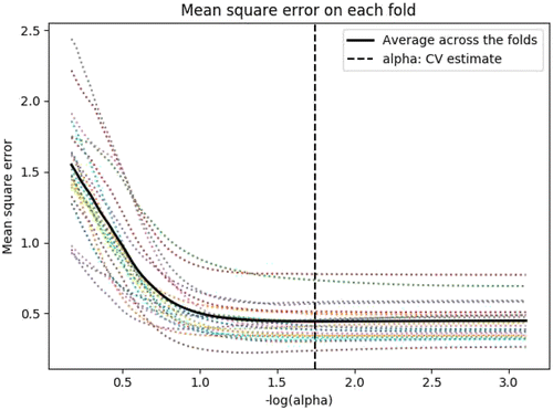
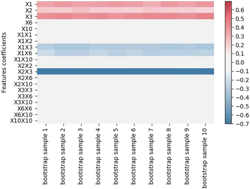
We feed this model to the LASSO algorithm in order to reduce the number of terms in the polynomial. Just as we use random forest algorithms to estimate models on many subsets of sample I to tune its hyperparameter (i.e., tree depth), we also obtain results from LASSO across multiple subsets of sample I using k-fold cross-validation (Figure 4; Appendix A).8 This procedure aids in tuning the hyperparameter for regularization. LASSO identifies seven terms {x1, x2, x3, x1 × x3, x1 × x6, x2 × x3, and x6 × x7} as the most important and robust predictors (out of 20). These seven are also robust predictors across subsamples (Figure 5) and bootstrap samples (Figure 6) in the data. The terms identified by LASSO are a superset of terms that form the DGP and the term x6 × x7 is again a false positive; it does not exist in the DGP. The last step within sample I is to run an OLS with these seven variables. The results of this OLS model are presented in Table 5 model 1. As one can observe, the results recover the DGP quite precisely and drop the spurious x6 × x7 interaction. Another OLS model is then run after dropping this spurious term and is presented in Table 5 model 2. Because our dependent variable Innovation is continuous between 0 and 1, we are dealing with a regression task. The accuracy of regression models is commonly measured by mean squared errors (MSEs). The prediction by random forest in sample I had an MSE of 0.96, and the combination of random forest and LASSO reduced the MSE to 0.43.

|
Table 5. OLS Models on Sample I
| Dependent variable: Innovation outcome | ||
|---|---|---|
| Variables | (1) | (2) |
| Weakness of IP protection | 0.38*** | 0.38*** |
| (0.03) | (0.03) | |
| Advertising intensity | 0.20*** | 0.21*** |
| (0.03) | (0.03) | |
| R&D intensity | 0.50*** | 0.50*** |
| (0.03) | (0.03) | |
| Litigation intensity | 0.02 | 0.02 |
| (0.03) | (0.03) | |
| Employee diversity | 0.01 | |
| (0.03) | ||
| Weakness of IP protection × R&D intensity | −0.27*** | −0.27*** |
| (0.03) | (0.03) | |
| Weakness of IP protection × litigation intensity | −0.43*** | −0.43*** |
| (0.03) | (0.03) | |
| Advertising intensity × R&D intensity | −0.66*** | −0.66*** |
| (0.03) | (0.03) | |
| Litigation intensity × employee intensity | −0.03 | |
| (0.03) | ||
| Constant | −0.02 | −0.02 |
| (0.03) | (0.03) | |
| Observations | 500 | 500 |
| R2 | 0.69 | 0.69 |
| Adjusted R2 | 0.69 | 0.69 |
| Residual standard error | 0.70 (df = 490) | 0.70 (df = 492) |
| F‐statistic | 122.59*** (df = 9; 490) | 157.95*** (df = 7; 492) |
Note. df, Degrees of freedom.
*p < 0.1; **p < 0.05; ***p < 0.01.
Stage 3: Building a Theoretical Explanation
At this point, the theorist must ask herself if these robust associations make theoretical sense. This is the abductive reasoning highlighted in stage 3. In our example, hopefully the theorist will spot that R&D intensity and advertising intensity could indeed be substitutes and that R&D intensity can be less useful if a firm operates in weak IP regimes. Less intuitively, weak IP regimes are positively associated weak innovation outcomes, and this effect is diminished when a firm engages in aggressive litigation. Should the theorist be well versed in the innovation literature, this pattern might suggest a logic of mutual benefit from spillovers among the firms within a sector. The theorist’s engagement with the context, in the form of literature reviews, interviews, or case analysis, may be helpful to stimulate the abductive process that produces a theory to account for the patterns in the data uncovered by the previous steps.
The abductive reasoning and the iteration between theory and data necessary at this stage require human expertise and judgment and cannot be left to an ML algorithm. The first output of this abductive reasoning is therefore a set of predictions to be tested in sample II by simply replicating out of sample. The six terms identified in OLS at stage 2.2, if replicated in the hold-out sample, instantiate this.
However, a more ambitious theoretical development is to construct out-of-pattern tests; these are patterns that were not necessarily found in sample I but are implied based on the explanations constructed to account for the patterns found in sample I. Thus, given the theory used to explain the patterns in sample I (e.g., R&D intensity and advertising intensity are substitutes and a weak IP regime lowers the value of R&D investment but may benefit the firm as long as it is not too litigious), what additional hypotheses could we make? If firms recognize some of the benefits of a weak IP regime, then an additional hypothesis might be that there should be a negative correlation between litigation intensity and weak IP regimes through some form of oligopolistic coordination. The specific theoretical explanation here is not relevant and we do not require the reader to endorse it; rather, the point is that such an additional out-of-pattern hypothesis test can be made in the first place.
In sum, the resultant stage 3 is a set of hypotheses, some of which are out of sample, whereas other are out of pattern. These hypotheses can now be tested in sample II (hold-out), with usual statistical significance reported.
Stage 4: Testing Hypotheses in Sample II
We test the hypotheses with a simple OLS regression in sample II, and the results are presented in Table 6. We add two control variables (age and size of the firm), which the theorist might feel are critical in light of prior studies. As one can observe in Table 6, the model is able to correctly identify the significant linear and interaction terms. In addition, as a test of out of pattern prediction, a hypothesis about correlation between IP regime strength and litigation intensity (controlling for other variables) also receives support (Table 7).
|
Table 6. OLS Model on Sample II for Testing Out-of-Sample Predictions
| Dependent variable: Innovation outcome | ||
|---|---|---|
| OLS coefficients | True coefficients | |
| Weakness of IP protection | 0.35*** (0.03) | 0.40 |
| Advertising intensity | 0.14*** (0.03) | 0.20 |
| R&D intensity | 0.50*** (0.03) | 0.50 |
| Litigation intensity | 0.01 (0.03) | 0.00 |
| Size (employees) | −0.01 (0.03) | 0.00 |
| Age of company | 0.01 (0.03) | 0.00 |
| Weakness of IP protection × R&D intensity | −0.27*** (0.03) | −0.30 |
| Weakness of IP protection × Litigation intensity | −0.39*** (0.03) | −0.30 |
| Advertising intensity × R&D intensity | −0.66*** (0.03) | −0.70 |
| Constant | −0.01 (0.03) | |
| Observation | 500 | 500 |
| R2 | 0.68 | 0.68 |
| Adjusted R2 | 0.68 | 0.68 |
| Residual standard error | 0.67 (df = 490) | 0.67 (df = 490) |
| F‐statistic | 117.48*** (df = 9; 490) | 117.48*** (df = 9; 490) |
Note. df, Degrees of freedom.
*p < 0.1; **p < 0.05; ***p < 0.01.
|
Table 7. OLS Model on sample II for Testing Out-of-Pattern Prediction
| Dependent variable: Litigation Intensity | |
|---|---|
| Weakness of IP protection | −0.33*** |
| (0.04) | |
| Advertising intensity | 0.02 |
| (0.04) | |
| R&D intensity | 0.01 |
| (0.04) | |
| Weakness of IP protection × R&D intensity | −0.02 |
| (0.04) | |
| Advertising intensity × R&D intensity | −0.03 |
| (0.04) | |
| Constant | −0.06 |
| (0.04) | |
| Observations | 500 |
| R2 | 0.11 |
| Adjusted R2 | 0.10 |
| Residual Std. Error | 0.92 (df = 494) |
| F Statistic | 12.17*** (df = 5; 494)) |
Note. df, Degrees of freedom.
*p < 0.1; **p < 0.05; ***p < 0.01.
These results are still correlational and do not support a causal interpretation. However, the theorist could of course use the standard methodologies that enable closer-to-causal inference in nonrandomized data, such as matching instrumental variables and fixed effects in both the theory-generating and testing phases wherever feasible. Because those concerns are distinct from ours (and well understood), we do not discuss those methods here. In addition to the results from the hold-out sample, we recommend full and transparent reporting of the analysis within sample I (used for pattern detection) and explicit recognition of the assumption that the two samples can be treated as independent samples drawn on the same DGP.
As a contrast, it is interesting to see what a simple exploratory regression approach would produce and how far it would get with the same data in terms of recovering the DGP. Clearly, an ad hoc search for significant (i.e., with p < 0.05) effects using only a simple linear model or by trying pairwise interactions or one quadratic term at a time is likely to be both time consuming and unlikely to find the DGP. In contrast, a brute-force approach may be to put all 11 variables, their 55 two-way interactions, and 11 quadratic terms (77 terms in total) into a kitchen-sink regression. In our example, such a procedure identified all six correct terms as being statistically significant but also identified two other terms as significant, although their true coefficients in the DGP are zero (i.e., false positives). Finally, one could run a stepwise regression on the 77 terms. In our example, this identified all six terms in the DGP correctly but also produced four additional terms (false positives) as significant, which did not exist in the DGP. This is because the naïve exploratory approach lacks the protection against overfitting that our procedure provides.
For this illustration, we consciously made two important simplifications: First, we assumed a particular set of coefficients in the DGP. However, independent of the specific parameters assumed previously, our arguments can be made with any arbitrary set of coefficients for this underlying DGP. In Appendix B, we show a generalization of this analysis to a larger variety of data generation processes (all of degree 2, but with randomly drawn coefficients).
We also illustrate a central tradeoff in algorithmically supported induction between interpretability and predictive accuracy. In this exercise, we evaluate the performance of our procedure (measured by the difference between the estimated and true coefficients in the DGP) while varying the number of features selected in step 2.1 and the amount of noise present in DGP. As expected from our reasoning about the tradeoff between interpretability and prediction accuracy, the procedure performs better as the number of features selected in step 2.1 (a measure of appetite for complexity in theorizing) increases and the amount of noise in the DGP (a measure of randomness versus pattern) decreases. Because our procedure begins without any knowledge of the underlying DGP, a useful benchmark is to compare it with random selection of hypotheses to be tested. The results show that our procedure performs significantly better (Appendix B, Figure B.1).

Notes. Each value corresponds to average Euclidean distance between B and B′ over 100 different DGPs. Smaller is therefore better.
Second, in this illustration, the DGP is designed to be a degree 2 polynomial. In management research, surveys of empirical papers (Hulland 1999, Haans et al. 2016) indicate that, in our field, most hypotheses feature a complexity up to quadratics and two-way interaction terms. In other words, the typical theory testing paper assumes (quite reasonably, given the importance of interpretability) that the DGP can be approximated by a linear function with one or two interaction terms at most. Our assumption about the DGP mirrors this. However, this might raise a legitimate concern that, when we approximate the underlying DGP with a degree 2 polynomial in stage 2.2, we (unsurprisingly) find a good fit.
In Appendix C, we therefore show what happens when the underlying DGP is of (a) higher degree, (b) lower degree, and (c) contains a variable not considered in the analysis while keeping the choice of a degree 2 polynomial in stage 2.2 of the algorithm-supported induction procedure. These illustrations cover the instances of oversimplification, undersimplification, and omitted variable bias that could occur while working with real data sets. In each of these cases, we evaluate our method in comparison with that of an analyst who conducts exploratory analysis without adopting procedures such as regularization and cross-validation that we propose in our procedure. We consider two types of exploratory analysts, namely, one who has either oversimplified or undersimplified the true degree of the underlying DGP or omitted a variable and does not use procedures to avoid overfitting or who has correctly identified the true degree of the underlying DGP but does not use procedures to avoid overfitting. We show that our method performs significantly better at identifying the underlying patterns compared with both these versions of exploratory analysis that differs from our procedure.
Discussion
In management and organization research, the use of large sample data for inductive and abductive theorizing rather than the test of hypotheses is rare. We suspect this may be partly the result of an incorrect (but, in our experience, widely held) premise that theorizing from data is necessarily restricted to qualitative data (Shah and Corley 2006, Locke 2015). As also noted by Glaser (2008), who helped lay the foundations for qualitative induction along with Strauss (Glaser and Strauss 1967), quantitative analysis can serve as a powerful stimulus to theory building. For instance, case control designs, which are popular in medical research, represent quantitative induction. In this method, a sample of cases that vary in their outcome of interest are statistically (i.e., algorithmically) analyzed to detect the correlates of the outcome in the data (Shadish et al. 2002, p. 128).
Building theory from data, whether with large or small samples, requires pattern detection and pattern explanation. The procedure for conducting algorithm supported induction that we have outlined in this paper can help scholars identify robust patterns in data, which can then become inputs to abductive theory construction (He et al. 2020). There are four key stages in this approach (Table 1): a split of the data into samples for pattern detection and hypothesis testing, the use of algorithms with tunable complexity to strike a well-considered balance between comprehension and prediction, the use of subsample replication to avoid overfitting even within the sample used for induction, and the imperative to create out-of-pattern tests in the hold-out sample. These four stages together constitute a new perspective on theory building from large-scale data, a meta-algorithm, none of whose components are necessarily new, but the integrated approach, we believe, is novel.
The insights that algorithm-supported induction produces may have long-term consequences for the way we craft theories in organization science; in the future, we may come to think of honest and sophisticated data mining as a sign of high-quality work (Bamberger 2018). At the very least, by complementing traditional inductive inference by humans, ML algorithms are likely to lend increasing prominence to theorizing from large sample data, as a manner of knowledge creation in our field. If there are concerns about the balkanization of theory, where a patchwork of sample specific theories emerge, it is useful to consider what their emergence implies: perhaps the existing more general theories are invalid or at least incomplete. Aggregation of results through meta-analysis of robust patterns is still the best-known methodology for building general insights from empirical research, and algorithm-supported induction helps, in our view, to produce the robust patterns (Hunter et al. 1982).
An instructive question to ask is whether the benefits of algorithm-supported induction require ML algorithms per se or even simpler and more familiar can suffice. First, as we already noted, familiar techniques such as OLS and logistic regression can be used for ML if the purpose is to fit data in a manner that optimizes the bias-variance tradeoff (Abu-Mostafa et al. 2012). Second, how our recommended procedure differs from the practice of a sophisticated user of exploratory regressions would depend on what that sophistication entails. If the user of exploratory regressions does all four stages of our procedure, then they are effectively replicating our procedure; depending on which step they diverge on. Table 2 shows what is lost.
As noted, most theory building from data in our field has been based on a limited number of cases, which may even provoke debates on replicability of results and transparency (Aguinis and Solarino 2019, Pratt et al. 2019). Thus, at this point, the theorist will naturally ask about the sample size required to be able to apply algorithm-supported induction. In principle, it is possible to detect robust patterns through ML with relatively small sample sizes. As we noted, in contrast to hypothesis testing, the key concern with induction through ML is overfitting and not statistical inference. For instance, one of the most widely known data sets for teaching ML, known as iris, contains only 150 observations of data with five variables. This is a data set for three species of iris flowers and has been used extensively to test and validate diverse ML algorithms and models in more than 100 academic papers (Dua and Graff 2017). In medicine, where generating cases is costly, ML techniques to work with small data sets have been developed through medical research (Shaikhina and Khovanova (2017) (where n = 56). A study by Jiang et al. (2009) is an instance of such an approach; they proposed modifications in existing ML algorithms for learning from samples as small as 24 cases (see also Zhou and Jiang 2003). Specific methods for small data sets include aggregation of regularized classifiers (Lu et al. 2010), robust sparse representation (Sami Ul Haq et al. 2012), and discriminant analysis (Chen et al. 2000).
The implication is that many things we have argued regarding algorithm-supported induction are in principle relevant even for smaller N methods of inductive and abductive theory building, such as the comparative case method (Eisenhardt 1989) or qualitative comparative analysis (Ragin 1987, 2000). The risks arising from neglecting to separate pattern detection and explanation in the multiple case method, and the risk of overfitting inherent in fitting multiple interactions to small samples in Boolean qualitative comparative analysis (QCA) are well known to its sophisticated practitioners, and they recommend careful measures to mitigate these (i.e., see a thoughtful discussion on these matters in Eisenhardt 1989, p. 545 and Fiss 2011). Our point in this paper simply is that where a sufficient number of cases exist relative to the parameters in the theory to be developed, algorithm-supported induction using ML may offer at least an alternate path to be explored.
Challenges and Opportunities
Having illustrated the promise of ML algorithms for inductive theorizing in organization science, it is equally important for us to point out the caveats. First, as we stressed at multiple points in the paper, ML algorithms today can support but cannot replace human judgment entailed in theory building through inductive and abductive reasoning. What is measured and how, and, critically, the explanation we propose for the observed pattern is still very dependent on human intuition and creativity, at least at the current state of development in the field of AI.
Second, ML itself is no magic bullet and involves many tradeoffs in choosing among suitable model families and algorithms. These choices are not straightforward given that no one algorithm fits all prediction tasks (there is no free lunch for optimizing loss functions, as Wolpert and Macready 1997 famously noted). Balancing the tradeoffs between ML algorithms requires the researcher’s ingenuity and domain knowledge to carefully evaluate the performance of the algorithm and compare this with others that are also potentially suitable. In general, we stress the importance of selecting algorithms that offer a high degree of interpretability (given that our purpose ultimately is the creation of theory) in stage 2.2 and procedures (such as regularization and cross-validation) that help mitigate overfitting in sample I. Within these parameters, many different algorithms may be useful, including familiar OLS and logistic regressions, and not only those we have illustrated in this paper (random forest and LASSO).
Third, algorithm-supported induction is not guaranteed to find interpretable robust patterns in the data, and falsification of a hypothesis constructed most carefully with algorithm-assisted induction can (of course) occur; this indicates that despite our best efforts, we stand defeated by sampling error or undetected flaws in measuring the data used for induction. That is also valuable learning for the theorist.9
Fourth, although ML methods rely on detecting associations, causal interpretations and conclusions require careful scrutiny. Although this is true for hypothesis testing in general (stage 4), the risk of biases in data leading to biased conclusions in the pattern detection phase is distinctly worth highlighting. Studies have demonstrated that, although ML algorithms are not inherently biased, they could under some conditions magnify biases already present in the training data (Kamishima et al. 2011, Zemel et al. 2013, Shrestha and Yang 2019). Such biases may constitute a more serious problem in ML than in traditional statistics because many ML models remain difficult to interpret and thus may have difficult-to-spot potential biases. For example, while training a neural network to aid a decision to award home loans, it is thus far not entirely possible to interpret how the weights of the network edges capture underlying lack of fairness in the training data with respect to the predicted decision. This is one more reason we strongly recommend against using black-box algorithms like deep learning for the purposes of algorithm-supported induction in stage 2.2, as well as reiterating that a causal theory that we develop in stage 3 to explain patterns obtained in stage 2 might nonetheless gain no support in stage 4 once properly tested with the techniques of causal inference.
Fifth, the use of ML techniques is fairly easy, but understanding the technical foundations for the advantages and disadvantages of the algorithms used is not, nor is keeping pace with rapid advances. Like any new tool, individual researchers should also be careful when importing methodologies from other fields. Organization and management researchers, like most social scientists, typically aspire to be sophisticated users rather than producers of statistical methodology. Identical to the adoption of other techniques developed by statisticians, the adoption of ML techniques in organization and management research requires not only familiarity and access to software that embeds these procedures but also a solid conceptual understanding of what the algorithms do and what they assume. This is made particularly challenging in the case of ML because of the rapid pace of developments in the field.
For instance, in recent years, the ML community has debated and made considerable progress in developing both fairer (Yao and Huang 2017) and more interpretable (Rudin 2014) algorithms. The subdomain of ML today referred to as interpretable AI is being developed for the sole propose of interpreting parts of very complex but effective ML models, such as deep neural networks (Guidotti et al. 2018, Samek et al. 2019). Interpretability is achieved in these models by (1) explaining the prediction based on local marginal effects—changes are made to particular inputs in either direction to observe the change in the prediction (LIME by Murphy et al. 2006); (2) abstract programming where learning is combined with query (Fischer and Krauss 2018); and (3) graphical plots and visualizations (Samek et al. 2019). Most of these methods to date focus on interpreting components of a complex and largely uninterpretable model and not necessarily explainability in intuitive human terms, and therefore, we do not think they are ready yet for use in theory generation by organizations researchers. In our field, we generally prefer imperfectly predicting but wholly comprehensible theories over perfectly predicting but only partially comprehensible theories. Nevertheless, given the rapid advances in this area, we encourage researchers to monitor progress on interpretable AI, because it may produce the next level of sophistication in algorithm-assisted theorizing.
Conclusion: Taming Pavlov’s Dog
ML algorithms such as supervised and unsupervised learning can be considered the descendants of Pavlov’s dogs: they are trained to develop associations between variables (e.g., establish the copresence of bell ringing and food) and then tested in their ability to predict the rest when presented with only some of the variables (e.g., will the bell ringing predict the presence of food?).10 However, these rudimentary learning mechanisms found (even) in our pets have enormous power and are at the heart of the current explosion of interest in ML. Admittedly, researchers in our field have already begun to exploit this power for data coding, data reduction, and support of traditional hypothesis testing by aiding causal inference. We offered an alternative perspective: treating a validated prediction model as a stylized fact opens up the path to theory development from data followed by theory testing in a mutually complementary manner, even possibly within the same study. As management and organization researchers, we have much to gain from understanding these opportunities.
All authors contributed equally. The authors thank Gino Cattani for excellent editorial guidance; two reviewers for insightful comments; seminar participants at the Vienna Strategy Conference for comments received on earlier versions of this paper; and Binod Bhattarai, Shijing Cai, Nina Geilinger, Thomas Gersdorf, Bibek Paudel, Prothit Sen, Bart Vanneste, and Ce Zhang for feedback.
Appendix A. Key Technical Concepts in ML
A.1. Loss Functions
In ML, model fitting occurs by minimizing a loss function. A loss function penalizes the discrepancy between the predicted outcome and the actual outcome in past data. OLS regression users will be aware that the loss function in OLS is the sum of squared error. There are several types of possible loss functions used in ML such as hinge loss, logistic loss, zero-one loss, and so on. A loss function can be minimized by rules (e.g., setting the derivative equal to zero and solving) or by search (e.g., gradient descent, Adam algorithm, Newton–Raphson) when the former is not feasible.
A.2. Bias-Variance Tradeoff
Statistical learning theory indicates that the complexity of a model selected to fit data has a U-shaped relationship with prediction error (Figure 1, left). Put differently, the prediction error initially decreases on increasing the model complexity and then increases afterward (Abu-Mostafa et al. 2012). The model is underfitting in the region before the inflection point and overfitting in the region after the inflection point. Underfitting produces prediction errors that are systematically biased (because they represent a systematic deviation from true model), whereas overfitting produces more variance (because the deviation is not systematic). The goal is to find the point where the model is sufficiently complex to accomplish the lowest prediction error possible given the constraints of the model family. Excessive model complexity and excessive sample dependence produce high prediction errors through overfitting.
A.3. Procedures to Mitigate Overfitting
Traditional statistical models use measures such as adjusted R2 in OLS and Akaike information criterion and Bayesian information criterion index in structural equation modeling to help mitigate the problem of overfitting through excessive model complexity. Bootstrapping offers a procedure to assess if a given model (typically used to test deductively derived hypotheses) is valid in subsamples (i.e., to check if there is excessive sample dependence). ML algorithms combine an automated model building process (which allows for complex functional forms) with procedures for mitigating both types of overfitting. First, regularization penalizes model fit for complexity. The intuition is similar to the use of adjusted R2 in OLS, although a wider variety of constraints on complexity can be adopted. For instance, LASSO, a popular ML algorithm, adds a penalty proportional to the absolute sum of the standardized coefficients in a linear regression model. This is comparable to minimizing the sum of squares with the additional constraint that the absolute sum of the standard coefficients should be less than or equal to a constant (e.g., 1). This type of regularization can result in sparse models with few coefficients. Coefficients of some variables with small effects can become zero and be eliminated from the model.
Second, cross-validation, which is used to solve the problem of excessive sample dependence, is closely related to the idea of a hold-out sample. In this method, we split the available data on Xs and Ys into random subsamples. Some of these subsamples are used to fit the model (or train it), whereas others are used to evaluate or test the fitted model for its predictive accuracy. Models that fit the training data sets well while also achieving good predictive accuracy in the test sets can be found by repeating this procedure a large number of times.
Cross-validation is an effective way of tuning hyperparameters– a set of parameters that describe a model family whose value is set before the learning process begins. For example, in the case of a random forest, hyperparameters include the number of decision trees in the forest and the number of features considered by each tree when splitting a node. Hyperparameter tuning relies on trying many different value combinations of hyperparameters and evaluating the performance of each, which can be effectively done by cross-validation, to find the hyperparameters that minimize the sum of prediction errors in different hold-out samples.
With these concepts, researchers can comprehend a large class of supervised ML models in terms of functional form complexity, loss functions, regularization strategies, and cross-validation techniques. One can also rely on an ensemble of models, averaging across many different models to improve prediction.
Appendix B. Algorithm-Supported Induction Illustrated with a Family of DGPs
In this section, we illustrate the algorithm-supported induction procedure with a more generalized DGPs than the specific example illustrated in the paper. We continue to use the same functional form for the DGP but allow for many more variants on coefficients:
B.1. Stage 1: Splitting the Sample
The first step for each sample is to divide the data randomly into sample I (pattern detection) and sample II (hold-out) samples of equal size (sample I = 500, sample II = 500).
B.2. Stage 2: Identifying Robust Associations Within the Inductive Sample
Within Sample I, we rely on a two-stage sequence of random forest to identify key predictors and then use LASSO to narrow down the subset of all second-order polynomials of these key predictors.
Step 2.1: We first used random forest to reduce the set of variables into consideration from 11 to xf_size. In our simulations, we varied the xf_size in the range {1, 2, 4, 6, 8, 10}.
Step 2.2: Based on the identified xf_size variables in step 2.1, we created a model with all possible degree 2 terms. This model is then fed to the LASSO algorithm in order to reduce the terms in the polynomial. We used k-fold cross-validation in order to identify the robust regularization parameter for LASSO in order to guard against overfitting.
Step 2.3: In the last step within Sample I, we run an OLS on a model comprising all the significant terms with nonzero coefficients identified in step 2.2 by the LASSO algorithms. The results indicate the inductively derived hypotheses to be tested in the deduction sample.
B.3. Stage 3: Testing Hypotheses in the Deduction Sample
Next, we run the same OLS model used in step 2.3 in sample I on sample II. As our algorithm-supported induction procedure is designed to identify robust associative patterns in data (instead of predicting Y with high accuracy), we calculated the performance of the procedure as the Euclidean distance between the vector of coefficients B originally used in the data generation process and the vector B′ returned by the OLS on the deductive sample. By design, the coefficients in B has at most 10 nonzero items. Moreover, B′ contains a nonzero coefficient if and only if a particular variable was identified as significant by the OLS in step 3, which also returned a nonzero coefficient. The Euclidean distance between the two vectors B and B′ is given by
The performance of our procedure for various configurations of noise_sigma and xf_size is presented in Figure B.1 (left). As we increase xf_size, the performance of the algorithm-supported induction procedure improves because the acceptable complexity of the inductive theorizer approaches true complexity.
To compare our results with the baseline, we also simulate the same procedure with a random induction procedure. In this alternative procedure, instead of using random forest and LASSO in steps 2.1 and 2.2, a random set of variables of equal size (that would have been selected by random forest and LASSO) are randomly selected from all linear and quadratic terms constructed from X. A model comprising exactly this set of terms is then fit into OLS in step 2.3. The performance of this procedure is displayed in Figure B.1 (right). The Euclidean distance values with this alternative procedure remains uniformly much higher compared with those in Figure B.1 (left). Moreover, performance fails to significantly improve as we increase xf_size for a fixed noise_sigma.
Appendix C. Algorithm-Supported Induction with Variations in DGP
We evaluate the performance of the algorithm-supported induction procedure under three different variations of DGP as follows:
Case 1: omitted variable case—where DGP contains a variable that is omitted from the data set available for algorithm-supported induction;
Case 2: oversimplification—where degree of polynomial selected in stage 2.2 of algorithm-supported induction is lower than the degree of DGP; and
Case 3: undersimplification—where the degree of polynomial selected in stage 2.2 in algorithm-supported induction is higher than the degree of DGP.
In each of these conditions, we compare the performance of our procedure with two different versions of what an exploratory analyst who does not use our procedure in terms of regularization and cross-validation procedure might do, namely (a) an exploratory analyst A who assumes degree 2 and investigates the DGP using linear regression with an exhaustive set of terms with at most degree 2, that is, with exactly 77 terms; and (b) an exploratory analyst B who assumes degree 1 and investigates the DGP using linear regression with only linear terms. The performance of these variations with respect to algorithm-supported induction procedure is compared in terms of Hamming distance of coefficients.
For all new DGP variants, the value of coefficients ( and ) remains the same as original DGP. In the Tables C.1, C.2, C.3 and C.4, we present the comparison in terms of Hamming distance for significance threshold p = 0.05. In the following, note that for original DGP, cases 1 and 2, exploratory analyst A correctly guesses the degree of functional form complexity but has no protection against overfitting, whereas exploratory analyst B does both oversimplify functional form complexity and has no protection against overfitting. For case 3, however, exploratory analyst A under simplifies functional form complexity and has no protection against overfitting, whereas exploratory analyst B correctly estimates the degree of functional form complexity but has no protection against overfitting. Results indicated that our procedure performs better than both types of exploratory analysts. Tables C.1, C.2, C.3 and C.4 indicate pairwise hamming distance between results from the two procedures being compared.
C.1. Original DGP: Case 1—Omitted Variable in Data Set Available for ASI
We try to recover the following DGP without specifying x12 in our induction procedure.
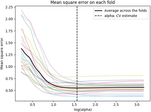
|
Table C.1. Comparison Based on p < 0.05 for Original DGP
| Hamming distance | ||||
|---|---|---|---|---|
| Exploratory analyst A (assumes degree 2) | Exploratory analyst B (assumes degree 1) | Our approach (random forest + LASSO) | True DGP | |
| Exploratory analyst A (assumes degree 2) | 0 | 10 | 7 | 7 |
| Exploratory analyst B (assumes degree 1) | 0 | 3 | 3 | |
| Our approach (random forest + LASSO) | 0 | 0 | ||
| True DGP | 0 | |||
C.2. Original DGP: Case 2—Oversimplification
We aim to recover the following DGP with selection of only degree 2 polynomial in step 2.2 in ASI (as in the illustration in the paper).
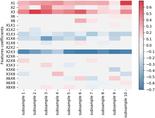
|
Table C.2. Comparison Based on p < 0.05 for Case 1 (DGP Has Omitted Variable)
| Hamming distance | ||||
|---|---|---|---|---|
| Exploratory analyst A (assumes degree 2) | Exploratory analyst B (assumes degree 1) | Our approach (random forest + LASSO) | True DGP | |
| Exploratory analyst A (assumes degree 2) | 0 | 5 | 1 | 2 |
| Exploratory analyst B (assumes degree 1) | 0 | 4 | 5 | |
| Our approach (random forest + LASSO) | 0 | 1 | ||
| True DGP | 0 | |||
C.3. Original DGP: Case 3—Undersimplification
Finally, we induce the following linear DGP with selection of degree 2 in step 2.2 of ASI.
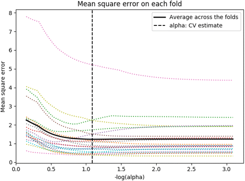
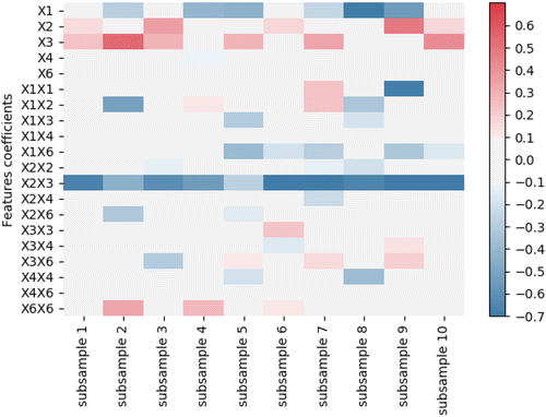
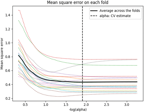
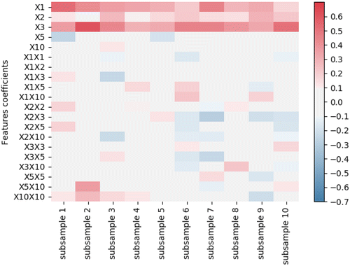
|
Table C.3. Comparison Based on p < 0.05 for Case 2 (DGP is Degree 3)
| Hamming distance | ||||
|---|---|---|---|---|
| Exploratory analyst A (assumes degree 2) | Exploratory analyst B (assumes degree 1) | Our approach (random forest + LASSO) | True DGP | |
| Exploratory analyst A (assumes degree 2) | 0 | 10 | 8 | 10 |
| Exploratory analyst B (assumes degree 1) | 0 | 2 | 4 | |
| Our approach (random forest + LASSO) | 0 | 2 | ||
| True DGP | 0 | |||
|
Table C.4. Comparison Based on p < 0.05 for Case 3 (Linear DGP)
| Hamming distance | ||||
|---|---|---|---|---|
| Exploratory analyst A (assumes degree 2) | Exploratory analyst B (assumes degree 1) | Our approach (random forest + LASSO) | True DGP | |
| Exploratory analyst A (assumes degree 2) | 0 | 7 | 7 | 7 |
| Exploratory analyst B (assumes degree 1) | 0 | 0 | 0 | |
| Our approach (random forest + LASSO) | 0 | 0 | ||
| True DGP | 0 | |||
Appendix D. Robustness Check of Algorithmic Induction Procedure against Different Algorithm Combinations
To demonstrate that our algorithmic induction procedure is not confined to a specific set of algorithms (random forest in the step 2.1 and LASSO in the step 2.2), we run our simulation by replacing random forest with gradient boosted regression and neural network-based feature selection in step 2.1 and RIDGE regression as a replacement for LASSO in step 2.2 without any changes in the underlying DGP.
Gradient boosting trains many models in a gradual, additive, and sequential manner: converting weak learners into strong learners. This method iteratively builds binary trees, that is, partition the data into two samples at each split node and in each iteration puts more weight on the errors from the earlier iteration (Breiman 2001). Neural network-based feature selection uses permutation importance to rank the importance of features, calculated after a model has been fitted. In this method, each feature x_i is randomly shuffled at a time, leaving the target and all other features in place, and the effect this has on the final prediction performance is noted (Yang et al. 2009). Such random ordering of variables is expected to reduce the predictive performance of the model. Worst performances result from the shuffle of the most important variables because we are in this case corrupting the natural structure of data. When a strong relationship is broken with our shuffle, we compromise what our model has learned during training, resulting in higher error. We illustrate the feature importance rank discovered by gradient boosting and neural network approach in Table D.1, which is qualitatively similar to the one discovered by random forest.
|
Table D.1. Set of Features Identified as Important by Different Algorithms in Step 2.1
| Top five selected features | |||
|---|---|---|---|
| Random forest | Gradient boosting regressor | Neural network | |
| Weakness of IP protection (x1) | × | × | × |
| Advertising intensity (x2) | × | × | × |
| R&D intensity (x3) | × | × | × |
| SGA expenses (x4) | × | ||
| Employee satisfaction (x5) | × | ||
| Litigation intensity (x6) | × | × | × |
| Employee diversity (x7) | |||
| Proportion of TMT with science degrees (x8) | |||
| Size (employees) (x9) | |||
| Age of company (x10) | × | ||
| CEO appeared in WSJ (x11) | |||
For stage 2.2 of our suggested approach, we require an interpretable model; hence, the choice of RIDGE regression-based feature selection (Marquardt and Snee 1975). RIDGE penalizes the model for the sum of squared value of the weights instead of sum of absolute values as in the case of LASSO. In total, we run our procedure with five new algorithmic combinations. Each of these combinations perform similarly in terms of predictive accuracy on sample II as displayed in Table D.2 with an MSE around 0.55. As shown in Table D.3, all these combinations of algorithms are able to correctly identify the true DGP and our baseline analysis (random forest plus LASSO).
|
Table D.2. Comparison of Various Algorithmic Combinations in Terms of Predictive Accuracy
| Accuracy: MSE (MAE for neural network) | MSE for the combination of the models in sample I | MSE in sample II | |
|---|---|---|---|
| Gradient boosted regression and LASSO | 1.41 | 0.43 | 0.56 |
| Gradient boosted regression and RIDGE | 1.41 | 0.43 | 0.54 |
| Random forest and LASSO | 0.96 | 0.43 | 0.54 |
| Random forest and RIDGE | 0.96 | 0.43 | 0.53 |
| Permutation-based neural network feature selection and LASSO | 0.67 | 0.43 | 0.56 |
| Permutation-based neural network feature selection and RIDGE | 0.67 | 0.43 | 0.54 |
|
Table D.3. Set of Features Identified as Significant by Different Combinations of Algorithms in Sample I at the End of Step 2.2
| Gradient boosted regression and LASSO | Gradient boosted regression and RIDGE | Random forest and LASSO | Random forest and RIDGE | Permutation-based neural network feature selection and LASSO | Permutation-based neural network feature selection and RIDGE | |
|---|---|---|---|---|---|---|
| Weakness of IP protection (x1) | × | × | × | × | × | × |
| Advertising intensity (x2) | × | × | × | × | × | × |
| R&D intensity (x3) | × | × | × | × | × | × |
| Litigation intensity (x6) | ||||||
| Weakness of IP protection (x1) × R&D intensity (x3) | × | × | × | × | × | × |
| Weakness of IP protection (x1) × litigation intensity (x6) | × | × | × | × | × | × |
| Advertising intensity (x2) × R&D intensity (x3) | × | × | × | × | × | × |
1 A third class of algorithms, reinforcement learning, is less relevant for our arguments here but is central to computational modeling of organizational adaptation by theorists; see Puranam et al. 2015 for a review.
2 For instance, OLS is a model family that assumes linearity in coefficients; decision trees assume a hierarchical interaction structure. Given the choice of a model family, ML procedures try to fit a model that optimizes the bias variance tradeoff.
3 Conventional approaches to building theory through inductive inference in small samples have corresponding ways to mitigate such bias, including triangulation (Lewis and Grimes 1999), search for theoretical saturation until no new insights can be gained through collection of novel data, and other ways to interpret data in grounded theory (Glaser and Strauss 1967).
4 The algorithms used in this paper have been well established and commonly applied in the field of ML. LASSO was developed in 1996 (Tibshirani 1996) and random forest in 2001 (Breiman 2001). The ideas on cross-validation were first discussed as early as around the 1930s (Larson 1931) and further advanced three decades later (Mosteller and Wallace 1963). Despite being not new, these algorithms and methods continue to form the core part of any ML textbook and ML exercise (Bishop 2006, Abu-Mostafa et al. 2012, Alpaydin 2014).
5 In this procedure, stages 2.1 and 2.2 can also accommodate unsupervised learning algorithms such as clustering or LDA to generate a robust set of interpretable patterns. The key difference is that the patterns would be identified not based on association of important features to a dependent variable but on dimension reduction principles.
6 It is important to note that in the context of ML, explainability and interpretability are often used interchangeably, although there is a technical difference (Lipton 2016). Interpretability relates to the extent to which a cause and effect can be observed within a phenomenon or system. In other words, it represents the ability to predict the outcome of a model, given a change in input or parameters. Explainability, in contrast, represents the extent to which the internal mechanism of a model can be explained in human terms. We use the term interpretability to cover both.
7 An implication is that when we apply an interpretability constraint in stage 2.2, it is useful for the researcher to show what would be the gain in predictive accuracy if a model with higher complexity (e.g., degree 3 polynomial instead of degree 2) was to be used in stage 2.2. This gain may be significant, but we might still choose to retain the simpler level of complexity because it is easier to interpret, but reporting the gain with the next higher level of complexity at least allows readers to see what is left on the table in terms of potential explanatory power.
8 In the LASSO model, we implemented regularization by varying the value of λ in the range [0.001,1] with 20-fold cross-validation (as show in Figure 3). The best value of α according to cross-validation performance was 0.0206, whose –log(α) is about 1.68. We used α of 0.0206 as our parameter. In the random forest, regularization was implemented by varying the depth of the trees and the number of trees that compose the random forest ensemble. In both these algorithms, regularization parameters were selected based on the cross-validation performance of the model.
9 Indeed, the result of a cross-validation exercise may reveal few robust patterns—a finding that is valuable in and of itself. Mullainathan and Spiess (2017) demonstrated that it was possible to build comparably predictive models of house prices across subsamples of data, but the predictors used in each sample differed substantially. In our view, this points (a) to the need for inductive theorists to focus on models that work reasonably well across a range of data segments although their predictive power may be lower and (b) to the acceptance that sometimes models that work across all data simply may not exist. If the latter is true, then the algorithms have saved the researcher from making an egregious error of overfitting in their inductive theorizing, although the result in terms of publishability may not be as uplifting.
10 Reinforcement learning, in turn, is the direct descendant of Thorndike’s cat, who learned through reinforcement (i.e., reward on success and punishment on failure) how to escape a cage.
References
- (2012) Learning from Data (AMLBook, New York).Google Scholar
- (2019) Transparency and replicability in qualitative research: The case of interviews with elite informants. Strategic Management J. 40(8):1291–1315.Google Scholar
- (2014) Introduction to Machine Learning (MIT Press, Cambridge, MA). Google Scholar
- (2016) Recursive partitioning for heterogeneous causal effects. Proc. National Acad. Sci. USA 113(27):7353–7360.Crossref, Google Scholar
- (2019) Generalized random forests. Ann. Statist. 47(2):1148–1178.Crossref, Google Scholar
- (2018) AMD—Clarifying what we are about and where we are going. Acad. Management Discovery 4(1):1–10.Crossref, Google Scholar
- (2014) Simultaneously discovering and quantifying risk types from textual risk disclosures. Management Sci. 60(6):1371–1391.Link, Google Scholar
- (2018) Perspective—Discovery within validation logic: Deliberately surfacing, complementing, and substituting abductive reasoning in hypothetico-deductive inquiry. Organ. Sci. 29(2):323–340.Link, Google Scholar
- (2013) Inference on treatment effects after selection among high-dimensional controls. Rev. Econom. Stud. 81(2):608–650.Crossref, Google Scholar
- (2006) Pattern Recognition and Machine Learning (Springer, New York).Google Scholar
- (2012) Probabilistic topic models. Comm. ACM 55(4):77.Crossref, Google Scholar
- (2017) Optimal classifier for imbalanced data using Matthews correlation coefficient metric. PLoS One 12(6):e0177678.Crossref, Google Scholar
- (2001) Random forests. Machine Learning 45(1):5–32.Crossref, Google Scholar
- (2011) Computational modeling for what-is, what-might-be, and what-should-be studies—And triangulation. Organ. Sci. 22(5):1195–1202.Link, Google Scholar
- (2017) Classical statistics and statistical learning in imaging neuroscience. Frontiers Neurosci. 11:543.Crossref, Google Scholar
- (2000) A new LDA-based face recognition system which can solve the small sample size problem. Pattern Recognition 33(10):1713–1726.Crossref, Google Scholar
- (2017) In search of new product ideas: Identifying ideas in online communities by machine learning and text mining. Creative Innovative Management 26(1):17–30.Crossref, Google Scholar
- (2012) Using natural language processing technology for qualitative data analysis. Internat. J. Soc. Res. Methodology 15(6):523–543.Crossref, Google Scholar
- (2010) Machine learning and rule-based automated coding of qualitative data. Marshall C, Toms E, Grove A, eds. Proc. ASIST Annual Meeting (John Wiley & Sons, Hoboken, NJ), 1–2.Google Scholar
- (2017) Using causal forests to predict treatment heterogeneity: An application to summer jobs. Amer. Econom. Rev. 107:546–550.Crossref, Google Scholar
- (1996) Crossroads—Describing differences in approaches to organization science: Rethinking burrell and morgan and their legacy. Organ. Sci. 7(2):191–207.Link, Google Scholar
- (2017) Machine learning repository. Accessed June 1, 2016, http://archive.ics.uci.edu/ml.Google Scholar
- (1998) Mediating the fact-value antinomy: Patterns in managerial and legal rhetoric, 1890–1990. Organ. Sci. 9(2):232–245.Link, Google Scholar
- (1989) Building theories from case study research. Acad. Management Rev. 14(4):532–550.Crossref, Google Scholar
- (2018) Deep learning with long short-term memory networks for financial market predictions. Eur. J. Oper. Res. 270(2):654–669.Crossref, Google Scholar
- (2011) Building better causal theories: A fuzzy set approach to typologies in organization research. Acad. Management J. 54(2):393–420.Crossref, Google Scholar
- (2014) The statistical crisis in science. Amer. Sci. 102(6):460–465.Crossref, Google Scholar
- (2008) Doing Quantitative Grounded Theory (Sociology Press, Mill Valley, CA).Google Scholar
- (1967) The Discovery of Grounded Theory (Weidenfeld & Nicolson, London). Google Scholar
- (2016) Scientific apophenia in strategic management research: Significance tests and mistaken inference. Strategic Management J. 37(1):167–176.Crossref, Google Scholar
- (2018) A survey of methods for explaining black box models. ACM Comput. Survey 51(5):1–42.Crossref, Google Scholar
- (2016) Thinking about U: Theorizing and testing U‐and inverted U‐shaped relationships in strategy research. Strategic Management J. 37(7):1177–1195.Crossref, Google Scholar
- (1985) An application of clustering for strategic group analysis. Strategic Management J. 6(1):55–73.Crossref, Google Scholar
- (2018) Product innovation rumors as forms of open innovation. Res. Policy 47(5):953–964.Crossref, Google Scholar
- . (2019) Topic modeling in management research: Rendering new theory from textual data. Acad. Management Ann. 13(2):586–632.Crossref, Google Scholar
- (2020) Resolving governance disputes in communities: A study of software license decisions. Strategic Management J. 41(10):1837–1868.Google Scholar
- (2007) Stylized facts, empirical research and theory development in management. Strategic Organ. 5(2):185–192.Google Scholar
- (2018) Analyst information discovery and interpretation roles: a topic modeling approach. Management Sci. 64(6):2833–2855.Link, Google Scholar
- (1999) Use of partial least squares (PLS) in strategic management research: A review of four recent studies. Strategic Management J. 20(2):195–204.Crossref, Google Scholar
- (1982) Meta-Analysis: Cumulating Research Findings across Studies (Sage Publications, New York).Google Scholar
- (2009) Mining extremely small data sets with application to software reuse. Software Practice Experience 39(4):423–440.Crossref, Google Scholar
- (2018) Multicollinearity: How common factors cause type 1 errors in multivariate regression. Strategic Management J. 39(8):2362–2385.Crossref, Google Scholar
- (2011) Fairness-aware learning through regularization approach.Google Scholar
- (2015) Prediction policy problems. Amer. Econom. Rev. Paper Proc. 105(5):491–495.Crossref, Google Scholar
- (1931) The shrinkage of the coefficient of multiple correlation. J. Edu. Psychol. 22(1):45.Crossref, Google Scholar
- (1993) An Introduction to Models in the Social Sciences (University Press of America, Lanham, MD).Google Scholar
- (2015) Deep learning. Nature 521(7553):436–444.Crossref, Google Scholar
- (1990) A dual methodology for case studies: Synergistic use of a longitudinal single site with replicated multiple sites. Organ. Sci. 1(3):248–266.Link, Google Scholar
- (1999) Metatriangulation: Building theory from multiple paradigms. Acad. Management Rev. 24(4):672–690.Crossref, Google Scholar
- (2016) The mythos of model interpretability. Accessed December 11, 2015, http://www.kdnuggets.com/2015/04/model-interpretability-neural-networks-deep-learning.html.Google Scholar
- (2015) Pragmatic reflections on a conversation about grounded theory in management and organization studies. Organ. Res. Methods 18(4):612–619.Google Scholar
- (2010) Regularized common spatial pattern with aggregation for EEG classification in small-sample setting. IEEE Trans. Biomedical Engrg. 57(12):2936–2946.Google Scholar
- (1991) Learning from samples of one or fewer. Organ. Sci. 2(1):1–13.Link, Google Scholar
- (1975) Ridge regression in practice. Amer. Statist. 29(1):3–20.Crossref, Google Scholar
- (2007) Weakly supervised learning for hedge classification in scientific literature. Carroll JA, van den Bosch A, Zaenen A, eds. Proc. 45th Annual Meeting Assoc. Comput. Linguistics (Association for Computational Linguistics, Prague, Czech Republic), 992–999.Google Scholar
- (1979) An emerging strategy of” direct” research. Admin. Sci. Quart. 24(4):582–589.Crossref, Google Scholar
- (1997) Machine Learning (McGraw-Hill, New York).Google Scholar
- (1963) Inference in an authorship problem: A comparative study of discrimination methods applied to the authorship of the disputed Federalist Papers. J. Amer. Statist. Assoc. 58(302):275–309.Google Scholar
- (2017) Machine learning: An applied econometric approach. J. Econ. Perspect. 31(2):87–106.Crossref, Google Scholar
- (2006) LIME: A coordination model and middleware supporting mobility of hosts and agents. ACM Trans. Software Engrg. Methodology 15(3):279–328.Crossref, Google Scholar
- (2000) Causal inference without counterfactuals. J. Amer. Statist. Assoc. 95(450):428–431.Google Scholar
- (1878) Deduction, induction and hypothesis. Popular Sci. Monthly 13:470–482.Google Scholar
- (1959) The Logic of Scientific Discovery (Basic Books, Oxford, UK).Google Scholar
- (2019) Editorial essay: The tumult over transparency: decoupling transparency from replication in establishing trustworthy qualitative research. Admin. Sci. Quart. 65(1):1–19.Google Scholar
- (2017) The effect of calorie posting regulation on consumer opinion: A flexible latent dirichlet allocation model with informative priors. Marketing Sci. 36(5):726–746.Link, Google Scholar
- (2015) Modelling bounded rationality in organizations: Progress and prospects. Acad. Management Ann. 9(1):337–392.Crossref, Google Scholar
- (1987) The Comparative Method (University of California Press, Berkeley). Google Scholar
- (2000) Fuzzy-Set Social Science . (University of Chicago Press). Google Scholar
- (2014) Machine learning, a probabilistic perspective. Chance 27(2):62–63.Crossref, Google Scholar
- (2014) Algorithms for interpretable machine learning. Macskassy S, Perlich C, Leskovec J, Wang W, Ghani R, eds. Proc. 20th ACM SIGKDD Internat. Conf. Knowledge Discovery Data Mining (Association for Computing Machinery, New York), 1519.Google Scholar
- , eds. (2017) Explainable AI: Interpreting, Explaining and Visualizing Deep Learning (Springer Nature, New York).Google Scholar
- (2012) A fast and robust sparse approach for hyperspectral data classification using a few labeled samples. IEEE Trans. Geosci. Remote Sensing 50(6):2287–2302.Crossref, Google Scholar
- (1959) Eight-move opening utilizing generalization learning. IBM J. 3(3):210–229.Crossref, Google Scholar
- (2002) Experimental and Quasi-Experimental Designs for Generalized Causal Inference (Houghton Mifflin, Boston). Google Scholar
- (2006) Building better theory by bridging the quantitative-qualitative divide. J. Management Stud. 43(8):1821–1835.Crossref, Google Scholar
- (2017) Handling limited datasets with neural networks in medical applications: A small-data approach. Artificial Intelligence Medicine 75:51–63.Crossref, Google Scholar
- (2014) Understanding Machine Learning: From Theory to Algorithms (Cambridge University Press, Cambridge, UK). Crossref, Google Scholar
- (2019) Interpreting interactions in linear fixed-effect regression models: When fixed-effect estimates are no longer within-effects. Strategy Sci. 4(1):25–40.Link, Google Scholar
- (2019) Fairness in algorithmic decision-making: Applications in multi-winner voting, machine learning, and recommender systems. Algorithms (Basel) 12(9):199.Crossref, Google Scholar
- (2019) Organizational decision-making structures in the age of artificial intelligence. California Management Rev. 61(4):66–83.Crossref, Google Scholar
- (1997) Crossroads—The virtues of closet qualitative research. Organ. Sci. 8(1):97–106.Link, Google Scholar
- (1996) Regression shrinkage and selection via the Lasso. J. Roy. Statist. Soc. B 58(1):267–288.Crossref, Google Scholar
- (2018) Big data methods. Organ. Res. Methods 21(3):525–547.Crossref, Google Scholar
- (2014) Big data: New tricks for econometrics. J. Econom. Perspective 28(2):3–28.Crossref, Google Scholar
- (2016) How to build an economic model in your spare time. Amer. Econom. 61(1):81–90.Crossref, Google Scholar
- (2018) Artificial intelligence in organizations: New opportunities for phenomenon-based theorizing. Acad. Managment Discovery 4(4):404–409.Crossref, Google Scholar
- (2015) Rejoinder: Moving the management field forward. Organ. Res. Methods 18(4):620–628.Crossref, Google Scholar
- (1997) No free lunch theorems for optimization. IEEE Trans. Evolution Comput. 1(1):67–82.Crossref, Google Scholar
- (2014) Semi-automatic content analysis of qualitative data. Accessed June 1, 2016, http://socqa.org/iConf2014.Google Scholar
- (2009) Feature selection for MLP neural network: The use of random permutation of probabilistic outputs. IEEE Trans. Neural Networks 20(12):1911–1922.Crossref, Google Scholar
- (2017) Beyond parity: Fairness objectives for collaborative filtering. Guyon I, Luxburg UV, Bengio S, Wallach H, Fergus R, Vishwanathan S, Garnett R eds. Advances in Neural Information Processing Systems, vol. 30 (Curran Associates, Red Hook, NY), 2921–2930.Google Scholar
- (2009) Case Study Research: Design and Methods (Sage Publications, Beverly Hills, CA). Google Scholar
- (2009) Using simulation to interpret results from logit, probit, and other nonlinear models. Strategic Management J. 30(12):1335–1348.Crossref, Google Scholar
- (2013) Learning fair representations. Dasgupta S, McAllester D, eds. Proc. 30th Internat. Conf. Machine Learning (PMLR, Atlanta), 325–333.Google Scholar
- (2003) Medical diagnosis with C4.5 Rule preceded by artificial neural network ensemble. IEEE Trans. Inform. Tech. Biomedicine 7(1):37–42.Crossref, Google Scholar
Yash Raj Shrestha is a senior researcher and lecturer at the chair of strategic management and innovation at ETH Zurich. He received a PhD in strategy from ETH Zurich. His research interests include new forms of organizing, organization design, and algorithms.
Vivianna Fang He is an associate professor of management at ESSEC Business School. She received her PhD in business administration from the George Washington University. Her research focuses on collaborative organizing in the context of new venture teams, research and development projects, and open-source software communities.
Phanish Puranam is the Roland Berger Chaired Professor of strategy and organization design at INSEAD. He received a PhD in management from the Wharton School at the University of Pennsylvania. His current research interests include nonhierarchical organizations, the design of informal organization, and organizational architectures that support self-assembling teams.
Georg von Krogh is a professor of strategic management and innovation at ETH Zurich. His long-term research program focuses on digital strategy, emerging technologies, and organizing, as well as the dynamics of open source software communities.

