Forgiveness in Vertical Relationships: Incentive and Termination Effects
Abstract
Two types of contractual solutions have been proposed for resolving incentive conflicts in vertical relationships: formal and relational (i.e., enforceable or not by third parties). Much is known about the optimal structure of formal contracts, but relatively little is known about the structure of relational contracts. We study a core feature of the latter: the conditions leading to continuation of the relationship, whose prospect gives relational contracts their force. We build a formal model of a vertical relationship between two parties that endogenizes the choice of the minimum performance necessary for continuation as a function of the values of contractibles, noncontractibles, and outside options. The model highlights a basic trade-off between providing strong incentives for the present (incentive effect) and safeguarding relationships for the future (termination effect). The stable relationships that follow from a more forgiving contract are more important under certain conditions (when a lot of value is jointly created by exchange partners, i.e., high contractible value, high noncontractible value, or unattractive outside options); however, strong incentives from a less forgiving contract are more important under other conditions (when a formal contract is insufficient and a relational contract is most important, i.e., high noncontractible relative to contractible value). We discuss implications for the choice of governance of interorganizational relationships.
1. Introduction
Vertical relationships are essential building blocks to students of economic organization (Williamson1975, Grossman and Hart1986, Poppo and Zenger1998). A fundamental concern is the incentive conflict that may arise between parties across adjacent steps of the value chain. Two different contractual solutions have been proposed: formal and relational. A formal contract is an agreement that is enforceable by third parties and under which the threat of external punishment provides incentives to cooperate (Williamson1985). In contrast, a relational contract is not enforceable by outsiders because they are unable to judge whether promises have been fulfilled; instead, it is sustained by the value of the future relationship (Macneil1978, Axelrod1984, Baker et al.2002). The incentive to cooperate stems from the threat of internal punishment—in particular, that one party will sever the relationship if the other party underperforms.
Many studies have analyzed the structure of formal contracts (e.g., Elfenbein and Lerner2003, Corts and Singh2004, Mayer and Argyres2004, Malhotra and Lumineau2011, Elfenbein and Lerner2012). Although relational contracts are no less frequent than formal ones (Macaulay1963), we know relatively little about their structure.1 Several scholars consider the ongoing nature of contracting relationships yet focus on prior rather than future interactions (e.g., Argyres et al.2007, Ryall and Sampson2009, Vanneste and Puranam2010). Other scholars do consider expected future interactions and how these affect cooperation between exchange partners (e.g., Heide and Miner1992, Jap and Anderson2003, Carson et al.2006, Poppo et al.2008); in that literature, however, the probability of future interactions is taken to be exogenous. That approach contrasts with the one taken here, in which the probability of the relationship continuing is an endogenous consequence of the relational contract design.
If potential punishment gives a relational contract its force, then one essential question about the structure of any relational contract is, which conditions would justify punishment? More concretely, where is the threshold that defines a party’s “underperformance”? This paper examines where the optimal punishment “trigger” should be set as a function of specific features of the contracting environment. We draw on an extensive literature pertaining to relational contracts (based on the theory of repeated games), although most work in that field does not address optimal contract structure and focuses instead on a different set of questions: existence and efficiency. The former is equivalent to asking, when will a relational contract arise—that is, under what conditions is it stable and enforceable (e.g., Green and Porter1984, Rotemberg and Saloner1986, Bull1987, MacLeod and Malcomson1989)? The latter asks, how efficient is a relational contract relative to (or in the presence of) other ways of governing a transaction (e.g., Baker et al.1994, 2002; Bernheim and Whinston1998; Rayo2007)?
As determinants of the optimal punishment trigger, the aspects of the environment that are central in contracting theories of vertical relationships are our focus. A major theme in this literature is that outsiders cannot objectively verify all outcomes of the relationship, which creates the need for relational contracts (Williamson1975, Macneil1978, Baker et al.2002). Following this literature, we explore the role played in such contracts by the value of so-called contractibles, noncontractibles, and outside options (Williamson1985, Grossman and Hart1986). First, that some outcomes are non-verifiable does not imply that all outcomes are, which means that formal and relational contracts may coexist (Baker et al.1994). Therefore, we examine the effect of contractible value: that portion of value that can be specified in a formal contract. Examples are delivery times, quantities, and measurable product attributes (e.g., the clock speed of a microprocessor or the dimensions of a machine part). Second, given the non-verifiability of certain outcomes, we also investigate the effect of noncontractible value: that portion of value that cannot be specified in a formal contract owing to inherent measurement difficulties. Examples include subjective quality (e.g., the image resulting from an advertising campaign, the commitment to share best practices, and continuous product innovation). Third, because terminating a relationship is relevant only when there are alternatives, we consider the value of outside options. The value of such an option is defined as the value of the best alternative relative to the value of the focal relationship. For instance, technological complementarity may allow a buyer to create more value with one supplier than with another.
We develop a formal model that endogenizes the choice of the punishment as a function of the values of contractibles, noncontractibles, and outside options. In this model, the trigger’s position is based on the minimum performance that must be met to avoid termination. Our model features two parties. One (Upstream) produces a good whose value depends on both effort and luck; the other (Downstream) decides, based on the good’s value, whether or not to continue the relationship. Because that value is but an imperfect measure of Upstream’s effort, Downstream’s decision is subject to error. Thus, it may happen that Downstream terminates the relationship even though Upstream worked hard. In the model, the optimal choice of performance threshold hinges on the trade-off between an incentive effect and a termination effect. On the one hand, a higher performance threshold from Downstream incentivizes Upstream to work harder (a positive effect); on the other hand, a harsher punishment shortens the duration of a potentially valuable relationship (a negative effect). The optimal performance threshold balances these two effects. We find that this threshold is decreasing in both contractible and noncontractible value (because these increase the termination effect relative to the incentive effect) and is increasing in the attractiveness of outside options (because that decreases the termination effect relative to the incentive effect). In short, we find that the more value is jointly created by exchange partners—through greater contractible and/or noncontractible value or through lesser outside option value—the lower the performance threshold. An additional result is that for constant total value, the greater the share of noncontractible value relative to contractible value, the higher the threshold. This is because that share decreases the termination effect relative to the incentive effect. Thus, when a formal contract cannot describe well the value created in an exchange, the relational contract is most important and will have a high performance threshold. In an extension, we show that the model’s main propositions are qualitatively unchanged if we instead assume that the performance threshold is exogenously fixed and that the decision variable is the probability of termination conditional on underperformance. In both cases, the key element is what the relational contract indicates about when to continue the relationship and, consequently, whether it is structured as a more demanding or a more forgiving contract.
Our main contribution is to show how this aspect of a relational contract’s structure—that is, the extent of its forgiveness—is optimally conditioned by the contracting environment, including elements known to be important in contracting theories of vertical relationships (e.g., contractible value, noncontractible value, outside options). We find two consequences to increasing the performance threshold: an incentive effect and a termination effect. The relative importance of each effect is altered by variations in these external factors, which accounts for variations in the performance threshold’s optimal level. Finally, to illustrate the model’s applicability, in the Discussion section we describe how our results can inform important questions regarding the choice of governance of interorganizational relationships.
2. Background
2.1. Theoretical Background
Relational contracts have different meanings across literatures. An economic interpretation, and the one followed here, is that relational contracts are agreements sustained by the value of the future relationship (Baker et al.2002). The basic idea is that a shared future enables cooperation because parties can be rewarded or punished tomorrow for things they do today (Axelrod1984). Game theory has extensively developed this idea. A well-established result is that cooperation can be individually optimal in a repeated game even if it is not optimal in a one-shot version of the same game (Friedman1971, Kreps et al.1982, Fudenberg and Maskin1986). In a one-shot game, current actions do not influence future payoffs. But a shared future—as arises in repeated games—provides the opportunity to reward and punish good and bad behavior, respectively, which incentivizes players to cooperate (Axelrod1984). An effective way of rewarding and punishing the actions of another player is a trigger strategy (Axelrod1984), whereby a player will cooperate in the next round only if the other player cooperates in the current round. Thus, a player’s defection triggers a punishment. Given their analytical tractability and intuitive appeal, trigger strategies underlie much of the theoretical work on relational contracts (Radner1981; Baker et al.1994, 2002). Consistent with theoretical predictions, empirical field studies find that the expectation of future interactions increases joint action (Heide and John1990); flexibility, information exchange, and problem solving (Heide and Miner1992); performance (Parkhe1993); and bilateral idiosyncratic investments (Jap and Anderson2003). Carson et al. (2006) find no effect on opportunism. Thus, a shadow of the future helps to align incentives between exchange partners.
A more sociological interpretation of relational contracts (and one that we do not follow here) refers to the norms of cooperation that may emerge over time between exchange partners (Granovetter1985, Gulati1995, Zaheer and Venkatraman1995, Puranam and Vanneste2009). The crucial distinction is that these works focus on the shadow of the past, not the future. A shared history facilitates social interactions, which in turn can lead to the establishment of cooperative norms such as trust (Gulati1995, Zaheer and Venkatraman1995, Uzzi1997). The shadow of the past and the shadow of the future may lead to the same outcome (e.g., cooperation), but they need not reinforce each other. For example, it might be harder to establish trust under expectations of future interactions because good behavior may be attributed to external factors (strong incentives) rather than internal factors (benevolence of exchange partner; see Malhotra and Murnighan2002). Thus, the two “shadows” are conceptually distinct. For this reason we restrict ourselves to relational contracts supported by expected future interactions.
It is typically assumed that relational contracts cannot be enforced by outsiders, and this is their key distinction from formal contracts. We do not refer to relational contracts as “implicit” contracts because doing so might create the false impression that relational contracts are vague. In fact, they can be written down and, in general, must be well understood to provide contracting parties the appropriate incentives. Scholars often analyze the design of a relational contract in terms of a fixed payment and, possibly, an additional bonus (e.g., Bull1987; MacLeod and Malcomson1989; Baker et al.1994, 2002). In this paper we focus on another key element of relational contracts: the performance threshold. To articulate this perspective clearly, our main model treats the payment as fixed so that we may restrict attention to the conditions for continuation. We also report on an extension to this model in which we allow for a bonus; the main results are unaffected.
Our approach is related to the models of Green and Porter (1984) and Rotemberg and Saloner (1986) on collusion and price wars in oligopolistic industries, which analyze a punishment trigger in terms of a price threshold. The market price dropping below that threshold could signal that some companies have violated the collusive agreement. Companies in the industry will retaliate by offering a lower price themselves (i.e., below the optimal collusive price). Similarly, we analyze a punishment trigger in terms of a performance threshold. Performance below this level constitutes cause for terminating the relationship. However, our model differs in several important respects. First, as noted previously, Green and Porter (1984) and Rotemberg and Saloner (1986) study the question of existence—in other words, the conditions under which a self-enforcing collusive agreement is feasible among members of an industrial cartel (horizontal relationships)—whereas we are concerned with the optimal structure of a relational contract between two parties in a bilateral vertical relationship and, in particular, with the optimal performance threshold that triggers punishment. Second, the results of Green and Porter (1984) and Rotemberg and Saloner (1986) depend in part on assumptions that are tailored to the context of an industrial cartel, so their results may not carry over to our context. Third, our key results concern the influence of exogenous parameters—contractible/noncontractible value and the value of the outside option—that do not feature in the other models at all. Finally, our notion of forgiveness is quite distinct from the one suggested by the limited-duration price wars in the other models: in our model, conditional on a single bad event, forgiveness is either forever or not at all. Forgiveness is embedded in the performance threshold, not in the duration of the punishment. Another related paper is Levin (2003), which considers a performance threshold as a punishment trigger in the context of bilateral relational contracts. We extend Levin’s work by investigating the optimal level of that performance threshold and how it varies as a function of a set of exogenous factors.
2.2. Empirical Background
Forgiving is a frequent phenomenon in real-world supplier relationships. Our theoretical analysis was originally inspired by extensive field research conducted at eight member companies of the Dutch Association for Purchasing Management (NEVI). The companies are active in different industries, including chemicals, telecommunications, basic materials, and transportation. Annual company revenues exceed €1 billion. All companies have international operations, although all of our 30 interview respondents (with job titles such as relationship manager, sourcing manager, and plant manager) were based in the Netherlands. Interviews lasted on average 70 minutes, with a minimum of 50 and a maximum of 100 minutes.
In our fieldwork we regularly saw a systematized version of forgiveness that had a natural connection to our model. Customers have complex performance expectations of their suppliers and use supplier rating systems to track performance and measure it on a unidimensional scale. These ratings are based on systematic checklists or questionnaires measuring multiple dimensions of supplier performance. For example, in one company, employees rated the vendor on five dimensions using questions including the following:
1. What is the defect rate in parts per million? (quality dimension)
2. What is the confirmed line item performance? (a measure of order performance; delivery dimension)
3. How does supplier’s cost position compare to the supply market? (cost dimension)
4. To what extent is the supplier flexible to changes in planning and ordering during the execution of deliveries for production and in lead-time reduction? (responsiveness dimension)
5. To what extent does the supplier provide proactively, and in a timely manner, technical road maps? (innovation dimension)
Based on these responses, the vendor was given a “traffic light” rating of green (performing), yellow (underperforming), or red (unacceptable). The rating, which corresponds to the unverifiable performance measure in our model, is a weighted average of multiple performance indicators that are largely unverifiable by outsiders. The buyer maintains a website where a supplier can log in to check its scores on the individual items and its aggregate score. Note that the buyer’s goal and expectation is a green level of performance from the supplier (and the supplier has been made well aware of this), but only a red rating results in supplier termination.
In another case, a similar system was in place, with A, B, C, and D ratings based on the aggregation of seven dimensions: safety, tidiness, quality, logistics, organization, communication, and cooperativeness. Even though these measures are not verifiable by outsiders, they are included in the supplier agreements (to which we had access). As Mayer and Argyres (2004) note, an unenforceable clause in a contract may still be useful to align parties’ expectations and their actions. The buyer shared each rating (individual items and aggregate score) with the supplier. The buyer’s goal, and the expectation shared with the supplier, was an A, but only a D was deemed unacceptable. In both cases from our fieldwork, that there is an intermediate zone of acceptable performance that is nonetheless below expectations indicates that forgiveness is built in to the supplier evaluation system.
In general, forgiveness is the tolerance of low performance. There are two specific ways of thinking about forgiveness. First, it can be seen as the deviation from desired performance that a party is willing to tolerate. If the deviation is too great, i.e., performance too low, the relationship is terminated. For instance, a professor who allows students to come to class up to 20 minutes late is more forgiving of lateness than a professor who sets the limit at 5 minutes. In the prior examples, each company has clear expectations about the desired performance level but must also define the acceptable deviation from that standard, i.e., choose the aggregate score that defines the lowest category and results in termination (i.e., a red light or a D score). This is the decision in our main model: a termination threshold, where a performance below that threshold results in termination.
A second way of viewing forgiveness is how often a party is willing to tolerate low performance, i.e., the propensity to enforce a predefined performance threshold. For instance, the professor who sets the maximum late arrival at five minutes but only enforces it in 50% of cases is more forgiving than the professor who sets the same threshold but enforces it in 100% of cases. In an extension, this is the version of forgiveness we model: a termination probability. There, performance can be either low or high, and low performance leads to termination with some probability. The results are qualitatively similar across both specifications.
3. Formal Model
3.1. Specification
Our model is based on Baker et al. (2002), which provides a useful foundation for thinking about vertical relationships based on relational contracts. Baker and colleagues address the relative efficiency of integration versus nonintegration as defined on the basis of asset ownership. In contrast, we focus on the optimal degree of forgiveness in relational contracts as indicated by the performance threshold triggering termination. Hence we do not use the asset ownership component of their model. Although asset ownership is certainly relevant, we treat it as a constant so as to articulate more clearly our own perspective on vertical relationships: a relational contract’s optimal degree of forgiveness.
We consider an Upstream and a Downstream party who can choose to trade with each other; both are risk neutral. In each period, Upstream produces a good by choosing a level of effort e ∈ [0, →) at cost c(e). Upstream’s cost is increasing in effort (∂c(e)/∂e > 0) at an increasing rate (∂2c(e)/∂e2 > 0). Upstream’s effort generates a stochastic value of the good, Q, for Downstream, where this value is continuous and QL ≤ Q < QH. Let ΔQ ≡ QH − QL > 0; then we can define Q ≡ QL + q(e)ΔQ, where q(e) is a stochastic function within [0, 1). Effort increases q(e) in a first-order stochastic dominance sense so that, on average, more effort leads to higher value.2 If Upstream exerts no effort, then we assume that the value of the good is minimum (Q = QL when q(0) = 0) and that the cost is zero (c(0) = 0).
We further assume that effort is observable only to Upstream and that no outsiders can verify the value of the good. It is therefore impossible to write an enforceable, formal contract on the input or output of the production process. Hence ΔQ captures all the elements that are noncontractible (owing to non-observability of effort or to non-verifiability of quality), and QL includes anything that can be addressed in a formal contract. Thus, ΔQ denotes noncontractible value and QL contractible value; their sum, QH, is total value.3
Downstream compensates Upstream through a combination of a fixed fee before production (w > 0)4 and the prospect of future business. Given our theoretical interests, the focus in this paper is on the latter. If the parties cannot agree on a compensation scheme, then they do not trade with each other and instead receive their outside option. We focus on those instances where the outside opportunities are less desirable than efficient trade yet more attractive than when Upstream has no incentive to perform (see Levin2003).5
In a one-time interaction, the up-front fee does not provide Upstream any performance incentive and leaves Downstream to bear the risk of moral hazard (i.e., Upstream providing insufficient or no effort). In this static game, Upstream and Downstream will not trade with each other given their outside opportunities. The prospect of repeated interactions, however, can incentivize Upstream and Downstream to trade—even when agreements are not enforceable. For Upstream, the cost of cheating (giving too little effort) now includes the possible lost value of the future relationship. So in the repeated game, Upstream and Downstream will trade with each other under certain conditions that we shall specify.
In the repeated game, Downstream faces an inference problem: If the value of the good is poor, did Upstream shirk, or was Upstream unlucky despite working hard? To provide incentives, in the first case Downstream would want to punish Upstream and terminate the relationship; in the second case, Downstream would want to reward Upstream and continue the relationship. Because effort is unobservable, Downstream cannot distinguish between these two cases. Hence Downstream specifies a minimum value: if realized value exceeds this level for a given period, then Downstream continues the relationship; otherwise, Downstream terminates the relationship. In short, one party (Upstream) expends effort and then the other party (Downstream) decides whether that effort’s outcome is sufficient to continue the relationship.
We can express this minimum value as QL + pΔQ, where p ∈ (0, 1) indicates the minimum proportion of noncontractible value that must be exceeded. We study the optimal threshold p∗, which provides a scale-free indicator of the relational contract. If the minimum threshold is not realized, then Downstream keeps the good and terminates the relationship, whereafter the parties receive their outside payments forever after. As in Klein et al. (1978) and Baker et al. (2002), we assume that Downstream can commit in advance not to renegotiate the contract in the event of underperformance—that is, its firing threat is credible. This assumption is motivated by the realization that if Downstream fails to carry through on its threats, then Upstream is unlikely to believe those threats in the future under a renegotiated contract (see also similar arguments in Fudenberg and Tirole1991 and Rabin1991). Hollow threats will not induce Upstream to exert effort. As a result, the relationship would be less valuable than the parties’ outside options.6,7
Let UO denote Upstream’s net present value of not entering the relationship (i.e., the value of the outside option), and let UR denote Upstream’s net present value of entering the relationship. The continuation probability is α ≡ P[q(e) > p], and we use a common discount factor λ ∈ [0, 1):
Likewise, let DO denote Downstream’s net present value of not entering the relationship, let DR denote Downstream’s net present value of entering the relationship, and define :
Then Upstream and Downstream will enter into the relationship if and only if their payoffs are higher than their outside options:
These boundary conditions imply that the wage must satisfy8
In the next section, we first explore the optimal effort level e∗ for Upstream and then Downstream’s optimal performance threshold, which is expressed as a proportion p∗ of noncontractible value.
3.2. Results
Upstream will choose optimal effort (e∗) to maximize its payoffs:
This gives the following first-order condition for the optimal effort level:
The left-hand side of this expression represents the marginal benefit of effort, and the right-hand side represents the marginal cost of effort. Upstream will choose effort such that the marginal benefit equals the marginal cost.
Downstream will choose the optimal threshold—expressed as a proportion p∗ of noncontractible value—to maximize its payoffs:
This leads to the following first-order condition for the optimal threat level:
The first term represents the marginal benefit of the threshold, and the second term represents its marginal cost. Hence, an increase in the threshold has two opposing effects on the relationship value for Downstream: an incentive effect and a termination effect ((dα/dp)λ(DR − DO)). In the appendix we show that the incentive effect is positive. It represents the increase in expected value resulting from greater effort. In equilibrium, if Downstream sets a higher threshold, then Upstream works harder, making it more likely that the good is of higher value. Thus the incentive effect is the marginal benefit of the performance threshold. The termination effect is the effect of an increase in the threshold on the probability of continuation. In equilibrium, an increase in the threshold makes it more likely that the relationship is terminated; hence a higher threshold reduces the expected duration of the relationship. If a higher threshold did not lead to more termination, then Downstream would increase the threshold because doing so would lead to more effort and would better safeguard the relationship. Because the outside option is less valuable (see Equation (3)), the termination effect is negative. Thus, the termination effect is the marginal cost of the performance threshold.
See the appendix for additional details and for the formal proofs of the propositions that follow. Our first proposition concerns Upstream’s optimal effort.
Optimal effort is increasing in the threshold atp = p∗ (∂e∗/∂p > 0).
The intuition behind this statement is as follows. In equilibrium, an increase in the threshold increases the marginal benefit of effort but does not affect its marginal cost. An increase in marginal benefit implies that effort is more critical for meeting the higher threshold (i.e., luck alone is less likely to be sufficient). It follows that optimal effort must increase. In other words, in equilibrium, the more likely the punishment, the less attractive the expected payoffs from exerting low effort. To avoid this outcome, Upstream exerts more effort; hence, its optimal effort increases with a stronger threat of termination.
We now turn to the propositions for Downstream’s optimal performance threshold. The optimal threshold is where the marginal benefit of the threshold equals its marginal cost or, equivalently, where the incentive effect equals the termination effect. Because of the termination effect, it is not always optimal to set a high threshold. The model points to a trade-off between providing strong incentives for immediate gains and maintaining the relationship for the future; one cannot have both.
We analyze this trade-off by examining how the optimal performance threshold is affected by contractible value (QL), noncontractible value (ΔQ), and the value of Downstream’s outside option (DO). To discover how the optimal threshold changes, we study how these exogenous variables affect the incentive and termination effects (i.e., the marginal benefit MB and cost MC). If the marginal benefit increases more (or decreases less) than the marginal cost, then the threshold will increase. Table 1 presents an overview of the results.
|

Table 1 Overview of Model Propositions
| Description | Incentive effect (MB) | Termination effect (MC) | Performance threshold (p∗) |
|---|---|---|---|
| Proposition 2: More contractible value, constant noncontractible value (∂p∗/∂QL|ΔQ) | Constant | Increases | Decreases |
| Proposition 3: More noncontractible value, constant contractible value (∂p∗/∂ΔQ|QL) | Increases | Increases more | Decreases |
| Proposition 4: More noncontractible value, constant total value (∂p∗/∂ΔQ|QH) | Increases | Decreases | Increases |
Proposition 2 addresses changes in contractible value while holding noncontractible value constant; conversely, Proposition 3 addresses changes in noncontractible value while holding contractible value constant. In both of these propositions, total value is allowed to change because it equals the sum of contractible and noncontractible value. In Proposition 4, we hold total value constant and consider changes in noncontractible value, which implies offsetting changes in contractible value. Hence, this proposition concerns the share of noncontractible relative to contractible value.
For constant noncontractible value, the optimal performance threshold is decreasing in contractible value (∂p∗/∂QL|ΔQ < 0).
The intuition for this result is as follows. An increase in contractible value increases the net present value of the relationship, making it more costly to terminate. Therefore, the termination effect is increasing in contractible value. The level of contractible value does not affect the incentive effect because contractible value does not depend on noncontractible effort; hence the incentive effect is constant and the termination effect increases. The marginal benefit is constant and the marginal cost increases, so the optimal threshold decreases.
The termination effect is negative because the relationship is more valuable relative to the outside option. Just as an increase in contractible value magnifies the termination effect, so does a decrease in the value of the outside option. Because a change in the outside option does not affect the incentive effect, the optimal threshold is increasing in the value of the outside option (∂p∗/∂DO > 0). In other words, for the optimal threshold, increasing contractible value is equivalent to decreasing the value of the outside option.
For constant contractible value, the optimal performance threshold is decreasing in noncontractible value (∂p∗/∂ΔQ|QL < 0).
An increase in noncontractible value increases the incentive effect because the former means that effort leads to higher expected payoffs in the current round. The termination effect also increases since the relationship becomes more valuable and hence termination more costly.
Which effect dominates? Let us compare two cases with equal amounts of noncontractible value but different amounts of total value. In case 1, noncontractible value accounts for a negligible share of total value; in case 2, noncontractible value accounts for almost the entire share of total value. An increase in noncontractible value leads to similar increases in the incentive effect in both cases. In case 1, however, the termination effect will hardly change relative to the change in the incentive effect because only a small part of the total value of the relationship is affected. The situation is reversed in case 2: relative to the change in incentive effect, the change in the termination effect will be much larger because a much larger part of the total value of the relationship is affected.
Given our focus on the shadow of the future, we are most interested in what the model tells us about relationships for which noncontractible value is important. As mentioned previously, we focus on instances where the outside opportunities are less attractive than efficient trade but more attractive than when Upstream has no incentive to perform. (In other words, absent noncontractible value, the parties would not enter the relationship because their outside options would be preferable.) We show in the appendix that for such relationships, changes in noncontractible value influence the termination effect more than the incentive effect. Hence an increase in noncontractible value raises the marginal cost more than the marginal benefit, so the optimal threshold will decrease.
For constant total value, the optimal performance threshold is increasing in noncontractible value (∂p∗/∂ΔQ|QH > 0).
Recall that Propositions 3 and 4 both relate to changes in noncontractible value but differ in what is held constant. In Proposition 3, contractible value is held constant so that a change in noncontractible value leads to a change in total value; in Proposition 4, total value is held constant so that an increase in noncontractible value leads to a decrease in contractible value. Thus Proposition 4 concerns the share of noncontractible value versus contractible value (for constant total value).
With an increase in noncontractible value, the incentive effect increases: the higher effort resulting from a higher performance threshold leads to more expected gains in the current round. In contrast, the termination effect decreases under these circumstances. Given constant total value, an increase in noncontractible value implies a decrease in contractible value. Therefore, the value of the best outcome per round remains constant while the value of the worst outcome decreases; hence the expected value of the relationship decreases. It thus becomes less costly to terminate the relationship. The marginal cost goes down and the marginal benefit goes up, so the optimal threshold will increase.
3.3. Alternative Specifications of the Model
We consider three alternative specifications of the model to assess the robustness of its results: an optimal threshold that maximizes total surplus (instead of the one that maximizes Downstream’s value), a bonus that is contingent on the value of the good (in addition to, or in lieu of, a fixed wage), and a stochastic decision rule for terminating the relationship (rather than a deterministic rule).
3.3.1. Total SurplusThe model described so far assumes that Downstream sets the optimal performance threshold to maximize its payoffs (DR). An alternative is to find the threshold that maximizes the joint payoffs for Upstream and Downstream. We define total surplus (SR) as
Now the optimal performance threshold p∗ is such that9
In the online appendix (available as supplemental material at http://dx.doi.org/10.1287/orsc.2013.0861), we derive the first-order condition. We find that the optimal threshold for maximizing only Downstream’s value is higher than the one for maximizing total surplus. The reason is that when maximizing total surplus, the incentive effect is lower (because it also reflects the costs that Upstream incurs when exerting more effort) and the termination effect is higher (because it accounts for the value lost not only by Downstream but also by Upstream). Hence the marginal benefit of the threshold decreases and the marginal cost increases. As a result, the threshold that maximizes Downstream’s value is higher than the threshold that maximizes total surplus.
Although the levels of the marginal benefit and cost change under the total surplus criterion, qualitatively, the analysis remains much the same. Indeed, it can be shown that the propositions addressing the optimal threshold (i.e., Propositions 2–4) hold when maximizing total surplus. In particular, the optimal performance threshold decreases if contractible value increases (Proposition 2) and decreases if noncontractible value increases (Proposition 3). Similarly, the share of noncontractible versus contractible value (Proposition 4) affects the optimal threshold in the same way regardless of which maximization criterion is applied.
3.3.2. BonusIn the model, Upstream receives a wage that is independent of the good’s value. We consider here a model in which, in addition to a wage, Downstream pays Upstream a bonus b if and only if the good’s value is above the critical threshold.10 In the online appendix, we provide Upstream’s and Downstream’s first-order conditions for this extension. The marginal benefit for Upstream’s effort now includes the additional expected bonus it will receive, while its marginal cost of effort stays the same. The marginal cost for Downstream’s threshold now takes into account the additional expected bonus it will pay in the current round. Its marginal benefit remains the same. Once again, the analysis is qualitatively unaffected even though the level of the marginal cost differs depending on whether a bonus is present. We can therefore use similar logic as before to show that all the propositions derived for a model without a bonus hold also for a model with a bonus.
3.3.3. Stochastic TerminationThe base model assumes that value is stochastic and continuous and the decision rule to terminate is deterministic—that is, terminate if performance is (at or) below the threshold but continue if it is above the threshold. An alternative is to assume that value is stochastic and discrete (i.e., QH with probability q(e) and QL with probability 1 − q(e)) and the decision rule to terminate is stochastic: if the value is QL, then Downstream terminates with probability < 1; if the value is QH, then Downstream continues with probability = 1. This scenario can be interpreted as Downstream playing a mixed strategy. In the online appendix, we show that the first-order conditions are almost identical to the first-order conditions for our basic model. Hence, we can use the logic from our basic model to re-derive all four of our propositions.
In sum, Propositions 1–4 hold across a number of different specifications, which suggests that our model captures a robust phenomenon. In the next section, we discuss the logic that unifies the different specifications.
3.4. The Incentive and Termination Effects
Our model highlights a trade-off between two opposing effects. The first is the incentive effect: a higher performance threshold incentivizes Upstream to exert more effort. If high performance is not required for the continuation of a relationship, then there is little incentive to work hard. But if future business is awarded on the basis of past outcomes, then Upstream has a strong motivation to perform. In such cases, future outcomes affect current actions. Opposed to this incentive effect is the termination effect: a higher performance threshold makes it more likely that a valuable relationship will be terminated. Punishing underperformance more harshly decreases the duration of the relationship, which offsets the incentive effect. The termination effect of a higher performance threshold is negative whenever the focal relationship is more valuable than the outside option. The existence of a termination effect implies that a more demanding or less forgiving relational contract (i.e., one with a higher performance threshold) is not necessarily better. Rather, the optimal performance threshold reflects a trade-off between providing strong incentives for the present and maintaining the relationship for the future.
Our model predicts differences in the optimal performance threshold depending on the amount of value from contractible versus noncontractible sources. By definition, contractible value can be captured in a formal contract. Noncontractible value cannot, and it is precisely in such cases that the promise of future business serves as an incentive. Our model predicts that the optimal performance threshold is decreasing in both contractible and noncontractible value (when either increases the total value of the relationship) but is increasing in noncontractible value when total value is held constant (i.e., when the share of noncontractible value relative to contractible value increases). So even when value can be specified in a formal agreement, it influences the relational agreement between two parties (see also Baker et al.1994, Bernheim and Whinston1998).
The intuition for these results can be found by examining how contractible and noncontractible value affect each of the incentive and termination effects. If the incentive effect increases relative to the termination effect, then the optimal performance threshold also increases. If the incentive effect decreases relative to the termination effect, then the optimal performance threshold falls. More contractible value by itself makes the relationship more valuable and thereby increases the termination cost. Yet more contractible value does not yield stronger incentives to produce noncontractible value, so the optimal performance threshold decreases with contractible value. By itself, more noncontractible value increases both the incentive and termination effects; incentives from threatening have more impact, and the relationship becomes more costly to terminate. When noncontractible value constitutes a large part of the relationship’s value—when the shadow of the future is most relevant—the termination effect will dominate the incentive effect. In other words, when a relational contract is most important (i.e., when a formal contract cannot describe well the value created in an exchange), the relational contract will be a demanding one (i.e., unforgiving).
Figure 1 illustrates these general results for the optimal performance threshold p∗ via arbitrary specific functional forms that conform to the general requirements for q(e) and c(e): q(e) = 1 − 1/(1 + x ⋅ 5e), where x is a random variable uniformly distributed in [0, 1); ; w = 0.45; UO = 4; DO = 4; and λ = 0.95. The figure shows that the optimal performance threshold is decreasing in noncontractible value (on the horizontal axis) and also in contractible value (on the vertical axis). For high values of either type, the optimal performance threshold is lower (p∗ < 0.05); for low values, that threshold is higher (p∗ > 0.35).
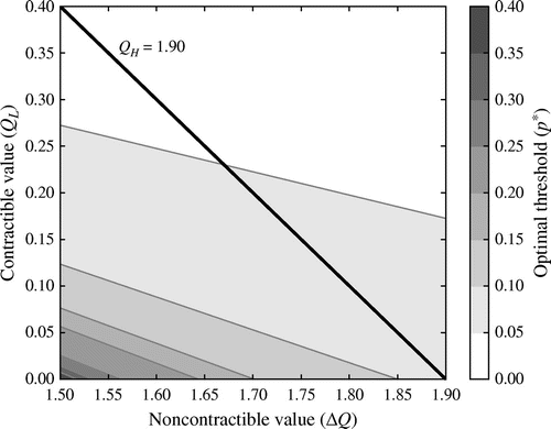
Figure 1 also shows how the optimal performance threshold varies in response to changes in the share of noncontractible relative to contractible value. Along the thick diagonal line that intersects the vertical axis at QL = 0.40 and the horizontal axis at ΔQ =1.90, total value is constant (QH = 1.90), but the share of noncontractible value increases from the vertical axis intersection to the horizontal axis intersection. Increasing the share of noncontractible value amplifies the incentive effect because it increases the gains from effort in the current round; however, it weakens the termination effect because the relationship becomes less valuable (in a given round, the best outcome is constant but the worst outcome worsens). Thus, more noncontractible value relative to contractible value leads to a higher performance threshold.
3.4.1. Effect of Wage on Optimal ThresholdWe provide here an additional analysis of the effect of the wage, a key incentive mechanism, on the optimal threshold (∂p∗/∂w). We illustrate that (1) the sign of this derivative is indeterminate, and (2) regardless of the sign, our propositions hold. We use the same specification as before: q(e) = 1 − 1/(1 + x ⋅ 5e), where x is a random variable uniformly distributed in [0, 1); ; UO = 4; DO = 4; and λ = 0.95 (see the online appendix for formal proofs and generic functions). Figure 2 shows four scenarios with differing levels of contractible and noncontractible value (I: QL = 0.0, ΔQ = 1.5; II:QL = 0.0, ΔQ = 1.9; III: QL = 0.4, ΔQ = 1.5; and IV: QL = 0.4, ΔQ = 1.9). This set of contractible and noncontractible values is such that the contractible value is not sufficient for the parties to enter into a relationship (but the sum of contractible and noncontractible values makes the relationship worth more than the outside options). For each scenario we analyze the entire wage range by increasing the wage in increments of 0.01 from the minimum to the maximum allowed value. The range of permissible wages varies across the scenarios because the value of the relationship differs.
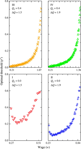
For the same production and cost functions, we observe all possible relationships between the wage and the optimal threshold. For the two upper plots, the optimal threshold increases with wage. For the two lower left plots, the optimal threshold initially decreases with wage, then is constant, and eventually increases. Thus, as suggested by the formal approach (see the online appendix), the relationship between wage and the optimal threshold is not unidirectional.
Regardless of the direction of the wage–threshold relationship, however, our main propositions hold. Proposition 2 states that the optimal threshold decreases in contractible value for constant noncontractible value. Proposition 3 indicates that the optimal threshold decreases in noncontractible value for constant contractible value. Proposition 4 says that the optimal threshold increases in the share of noncontractible value for constant total value. Taken together, this implies the following for the optimal threshold for the different scenarios:
• because the level of contractible value is greater in scenario III and the level of noncontractible value is the same (Proposition 2).
• because the level of noncontractible value is greater in scenario II and the level of contractible value is the same (Proposition 3).
• because the share of noncontractible value is greater in scenario II and the level of total value is the same (Proposition 4).
• because the level of noncontractible value is greater in scenario IV and the level of contractible value is the same (Proposition 3).
Figure 3 illustrates these propositions. It shows the optimal threshold for the different scenarios for the wages that are permissible in all scenarios. In other words, Figure 3 shows a subset of the data of Figure 2. For the same wage, we see that our propositions hold such that . Scenario I (▽) is above scenario II (+), is above scenario III (×), and is above scenario IV (△).
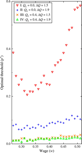
In Figure 3 some wages create more value than others. An optimal wage is such that no other wage from the range of permissible wages creates more value in the relationship. The propositions are derived for any arbitrary wage that causes both parties to enter the relationship voluntarily. Thus, regardless of the value of the wage (provided that the boundary conditions are met; see (4)) or the wage’s relationship with the optimal threshold, the propositions hold.
4. Discussion
The key decision variable in our model is the performance threshold specified by the relational contract, a value (at or) below which the relationship is terminated. This decision variable can be thought of as establishing either a more forgiving contract (lower threshold or termination probability) or a less forgiving one (higher threshold or termination probability). In this section, we relate our findings to management theory and practice. First, we highlight that forgiving is important, beneficial, and frequent.
Forgiving is important when a vertical relationship (partly) depends on a relational contract, which Macaulay (1963) suggests is often the case. By definition, a relational contract is unenforceable by outsiders. Instead, the incentive to cooperate comes from the threat of internal punishment—in particular, the breaking of the relationship if the other underperforms. Therefore, a fundamental question about the structure of any relational contract is, what conditions justify punishment? Or conversely, what conditions justify forgiveness?
Forgiving is beneficial when actions relate imperfectly to outcomes. In groundbreaking work, Axelrod (1984) discovered that in repeated prisoner’s dilemmas, a simple tit-for-tat strategy—start with cooperation and then do whatever the other player does—was most successful. Soon, however, it became clear that this finding did not generalize to settings with noise (equivalent to “luck” in our model setup), i.e., where an outcome is an imperfect indicator of what the other did. An unintended defect outcome would trigger retaliation in a tit-for-tat strategy. A more forgiving strategy, i.e., one that does not immediately play defect after the other defects, outperforms tit-for-tat in a noisy environment (Bendor et al.1991, Nowak and Sigmund1992, Kollock1993). Thus forgiveness implies a tolerance for bad outcomes. To the extent that in vertical relationships actions imperfectly relate to outcomes, forgiveness is beneficial. Finally, forgiving is a frequent phenomenon in real-world supplier relationships, as also observed in our fieldwork.
Given the importance of forgiveness, how might researchers test our theory and managers apply it? We offer one direction here: if (1) governance structures differ in terms of their levels of forgiveness and if (2) relationship value-added and share of noncontractible value influence the optimal level of forgiveness, then (3) relationship value-added and the share of noncontractible value will affect governance structures, all else being equal. We discuss these points in turn.
On the first point regarding the decision variable, we conjecture the degree of forgiveness to depend on the nature of the relationship. Supplier relationships come in many shades, including—in increasing intensity of collaboration—arm’s-length relationships, nonequity alliances, equity alliances, and joint ventures (Yoshino and Rangan1995). We speculate that higher degrees of collaboration between a buyer and supplier will be associated with higher levels of forgiveness. More generally, the organization of vertical relationships can be described on a continuum with markets and firms as endpoints (Stinchcombe1985, Powell1987, Hennart1993). Firms tend to be more forgiving than markets in the sense that firms have a higher tolerance of bad outcomes before relationships are terminated (Williamson1985, Powell1987, Eccles and White1988). We anticipate that this association holds not just for the endpoints of the continuum but also for intermediate forms, so that more firm-like external relationships are more forgiving than more market-like external relationships. For example, a nonequity alliance would be more forgiving than an arm’s-length relationship but less so than an equity alliance.
On the second point, regarding the main exogenous parameters in our model—total value, contractible value, and noncontractible value—we see two possible approaches.11 One is to look for direct empirical equivalents of these constructs. The other, which is possibly easier for measurement, is to think in comparative terms. Here, we discuss how this might be accomplished through a simple transformation of our parameters that preserves all of the model’s key propositions.
Specifically, we can define the share of noncontractible value as the fraction of value created in the relationship that comes from noncontractible sources, or ΔQ/QH. And we can define relationship value-added as the ratio QH/dO, where dO represents the per-period value of the outside option. The optimal threshold is increasing in the share of noncontractible value (from Proposition 4) and decreasing in relationship value-added (based on Propositions 2 and 3, and as we further illustrate in the online appendix). The share of noncontractible value might be associated, for example, with the nature of the product. If it is a service, it might be difficult for third parties to verify outcomes of the relationship because they are mainly intangible (Levitt1981). If the product is a tangible, physical good, verification by a third party becomes easier so that the share of noncontractible value is lower.12 Relationship value-added is closely associated with Dyer and Singh’s (1998) “relational rents.”
Combining the first point (on forgiveness and governance structures) and the second point (on relationship value-added/share of noncontractible value and forgiveness) then suggests that a high share of noncontractible value is associated with less forgiving governance structures (e.g., arm’s-length relationship) and high relationship value-added with more forgiving governance structures (e.g., equity alliances), all else being equal. When the share of noncontractible value is high and relationship value-added low (or vice versa), a governance structure with a more intermediate level of forgiveness might be preferred (e.g., nonequity alliance).
We highlight the following contributions. Our main contribution is to analyze how a critical aspect of any relational contract—the extent of its forgiveness—is influenced by the contracting environment. Existing literature has paid more attention to the structure of formal than relational contracts, despite the latter being ubiquitous (Macaulay 1963). Based on the model, we find that less forgiveness—through a more demanding performance threshold—has two consequences: an incentive effect (so that the other party works harder) and an opposing termination effect (so that it is more likely that the relationship will be terminated). We find that the optimal performance threshold is decreasing in both contractible and noncontractible value and is increasing in the share of noncontractible value relative to contractible value and value of the outside options.
A second contribution is to the literature on vertical relationships. These relationships come in many gradations and are usefully thought of as lying on a continuum with markets and firms as endpoints (Stinchcombe 1985, Powell 1987, Hennart 1993). Because most relationships are of an intermediate form (Powell1987, Hennart1993, Zenger and Hesterly1997), one cost of focusing on pure forms is a deficient understanding of the many organizational arrangements that are not pure (Stinchcombe 1985). Collectively, this research suggests that we should view governance forms as being distributed on a continuum or, at the very least, that we consider the discrete forms observed in practice to be correlated with some underlying, continuous latent variable. Our treatment of a continuous governance mechanism—the extent of forgiveness—offers a natural way, going forward, to theorize about this latent variable and the many relationships occupying the interior of the continuum, which include arm’s-length relationships, nonequity alliances, equity alliances, and joint ventures (Yoshino and Rangan1995).
Prior literature on vertical relationships has highlighted the importance of expected future interactions on cooperation, also known as the shadow of the future (e.g., Heide and Miner 1992, Jap and Anderson 2003, Carson et al. 2006, Poppo et al. 2008). We add to this literature by highlighting an important trade-off in how the shadow of the future shapes incentives in vertical relationships. When future interactions are expected with certainty (i.e., when forgiveness for underperformance is automatic), they provide no incentive. However, too-strict termination conditions (i.e., no forgiveness at all) may result in the loss of a valuable relationship. The optimal contract must balance these conflicting concerns.
We note the following limitations. As for any model, we faced a decision about what to include and what to exclude. We have chosen to present a fairly parsimonious model. Although this aids clarity and enables us to identify the key mechanisms, it also means that certain empirical phenomena are not readily represented in our model. For example, we focus on one-sided production (i.e., the upstream party produces), whereas some relationships may involve joint production. Relatedly, we focus on the moral hazard of the upstream party (e.g., effort level). In practice, there might also be the potential that Downstream fails to live up to its obligation, such that moral hazard is double-sided. Finally, the model considers each supply relationship in isolation, though spillovers may exist between relationships (Argyres and Liebskind1999, Frank2013). We see these as useful extensions for future research.
We suggest several further avenues for future research. The first avenue is direct empirical testing of the model’s implications as discussed above. Second, our model can be extended to horizontal relationships. Those that rely on one-sided production are easily represented in the current model. Relationships involving two-sided production would require that the model be refined. Third, we argue that the degree of forgiveness is an important governance mechanism in vertical relationships between firms. An important question is how different governance modes—arm’s-length relationships, nonequity alliances, equity alliances, and joint ventures—affect forgiveness. As discussed earlier, we suspect that the degree of forgiveness is higher in joint ventures than in alliances and higher in alliances than in arm’s-length relationships. Future research needs to establish whether this is indeed the case, and if so, why. Fourth, we have focused on vertical relationships between firms, but such relationships also occur within firms. Relationships within firms tend to be more forgiving than relationships between firms in the sense that within firms there is a higher tolerance for bad outcomes before relationships are terminated (Williamson 1985, Powell 1987, Eccles and White 1988). Future research can establish to what extent our predictions about between-firm relationships hold for predictions about within- versus between-firm relationships.
5. Conclusion
Our theory formalizes the notion of forgiveness in the context of a relational buyer–supplier contract and highlights the double-edged nature of forgiveness in these contracts. More forgiveness is valuable because it leads to more stable relationships that are less likely to be terminated because of accidental underperformance. However, more forgiveness also dampens the supplier’s effort incentives, since a less demanding performance threshold is more easily met. Our fieldwork and discussion indicate two ways that different degrees of forgiveness might be implemented in practice. One is by choosing a more or less stringent performance threshold, such as in the supplier evaluation systems that we observe in our fieldwork. The other is by choosing the degree of buyer–supplier integration. In the discussion, we conjecture that a more arm’s-length relationship is inherently a less forgiving one, whereas a relationship that more closely resembles vertical integration is inherently more forgiving. Our theory therefore has implications not only for contract design but also for the design of interorganizational relationships. We believe that further analyses through the lens of forgiveness could yield important insights into such relationships.
Supplemental Material
Supplemental material to this paper is available at http://dx.doi.org/10.1287/orsc.2013.0861.
The authors appreciate the helpful comments of Afonso Almeida Costa, Sendil Ethiraj, Isabel Fernandez-Mateo, Gerry George, Javier Gimeno, Sameer Hasija, Toby Kretschmer, Gwendolyn Lee, Ioana Popescu, Phanish Puranam, Mari Sako, Jasjit Singh, Kannan Srikanth, Peter Zemsky, the Management Science and Innovation reading group at the University College London, seminar participants at INSEAD and the Rotterdam School of Management, and attendees of the Academy of Management Conference and the Winter Strategy Conference. They are grateful for the insightful and constructive comments of senior editor Nick Argyres and the reviewers. The authors also appreciate the many people who contributed their time so generously during their fieldwork. They thank Sicco Santema and the Dutch Association for Purchasing Management (NEVI) for making that possible.
Appendix
We present proofs of all propositions. Upstream sets optimal effort (e∗) to maximize its net present value of entering the relationship (UR). If c(e) and α(e) are twice differentiable, then the first-order condition follows from
The second-order condition is ∂2UR/∂e2 < 0, which holds for the standard case of increasing marginal costs (∂2c(e)/∂e2 > 0) and decreasing marginal returns (∂2α(e)/∂e2 < 0; i.e., more effort increases the continuation probability at a decreasing rate).
Downstream sets the optimal threshold p∗, expressed as the proportion of noncontractible value, to maximize its net present value of entering the relationship (DR). Our results hold for any wage as long as, for each party, the relationship is more attractive than the outside option (see (4)). Thus, the model allows for bargaining over the wage between Upstream and Downstream, while Downstream selects the threshold. Provided that the second-order condition holds, then the first-order condition follows from
By (14), the threshold (p) affects the marginal benefit of effort (e) and not the marginal cost. We show below that an increase in the threshold increases the marginal benefit. As a result, ∂e∗/∂p > 0.
From (16) it follows that and dα/dp have the opposite sign. We can write these terms as
Because , ∂α/∂p < 0, and ∂α/∂e∗ > 0, it follows that ∂e∗/∂p > 0 (for otherwise, and dα/dp would have the same sign).
Because ∂e∗/∂p > 0 (see Proposition 1), by (16) we have and dα/dp < 0. Thus the left-hand side in (16) is the marginal benefit of the threshold p, or the incentive effect; the right-hand side is the marginal cost of the threshold, or the termination effect.
It follows that an increase in contractible value QL increases the marginal cost (through DR) but does not affect the marginal benefit (because noncontractible value ΔQ is constant). Therefore, ∂p∗/∂QL|ΔQ < 0.
Next we show that ∂p∗/∂QL|ΔQ = −∂p∗/∂dO, where dO is the per-period value of Downstream’s outside option (i.e., dO ≡ (1 − λ)DO). Using , we define the implicit function F1, based on the first-order condition (16):
Applying the implicit function theorem yields
Thus, ∂p∗/∂QL|ΔQ = −∂p∗/∂dO if ∂F1/∂QL = −∂F1/∂dO, which is the case:
From (16) it follows that an increase in noncontractible value ΔQ increases both the marginal benefit and the marginal cost (through DR) of the threshold. To determine the overall effect on the threshold, we define the implicit function F2, based on the first-order condition (16):
The second-order condition implies that
Applying the implicit function theorem now yields
Since ∂F2/∂p < 0 (by 22), ∂p∗/∂ΔQ|QL has the same sign as ∂F2/∂ΔQ, which has the opposite sign of ∂((DR − DO)/ΔQ)/∂ΔQ (because dα/dp < 0 by (16)). Then, since
Because Downstream’s value of the relationship (DR) if Upstream has no incentive to perform (e = 0) is less than Downstream’s outside option (DO), it follows that
Hence, by (24), ∂((DR − DO)/ΔQ)/∂ΔQ > 0, and therefore ∂p∗/∂ΔQ|QL < 0.
Given constant total value (QH), an increase in noncontractible value (ΔQ) is equivalent to a decrease in contractible value (QL); hence ∂p∗/∂ΔQ|QH and ∂p∗/∂QL|QH have the opposite sign. Since ΔQ ≡ QH − QL, it follows from the first-order condition (see (16)) that
We can now write , whence an increase in contractible value (QL) decreases the marginal benefit and increases the marginal cost (through DR). Therefore, ∂p∗/∂QL|QH < 0 and ∂p∗/∂ΔQ|QH > 0.
1 In this paper we are concerned with relational contracts (which differ from formal contracts in that they are not enforceable by third parties) as distinct from implicit contracts (which differ from formal contracts in that their terms are imprecisely defined or even unspoken).
2 We use a generic functional form q(e) to provide as general results as possible. The specific form of q(e) will affect the optimal threshold, but it will not affect our propositions, which have to do with how that threshold responds to changes in contractibles, noncontractibles, and outside options.
3 Following Baker et al. (2002), we acknowledge the importance of formal contracts but do not model them explicitly because our main interest is in agreements sustained by the shadow of the future. Although we discuss several important interactions between formal and relational agreements, our approach does not allow us to cover them all. For more on such interactions, see Baker et al. (1994) and Bernheim and Whinston (1998).
4 This is equivalent to a guaranteed payment after production.
5 If outside opportunities are always less desirable, then it is never optimal to break the relationship. Although such cases may exist, they are irrelevant to a model that seeks to characterize the optimal performance threshold for breaking the relationship.
6 According to the well-known Folk Theorem (Fudenberg and Maskin1986), repeated-game models often admit many possible equilibria. We focus on forgiveness in our model because of its empirical relevance. See the concluding section for examples.
7 Some versions of efficiency wage theory—specifically, the shirking model (Shapiro and Stiglitz1984)—involve contracts similar to the one we model here. However, our model is different in at least two key respects. First, efficiency wage theory is more a general equilibrium theory of the labor market than a theory of bilateral contracting. Second, the efficiency wage literature does not consider the question of the optimal degree of forgiveness that is the focus of our model.
8 We treat the wage as exogenous because our theoretical interest is in the degree of forgiveness. For an analysis of the wage, see the discussion in §3.4.1.
9 The total surplus could be maximized in one of two ways. One is that a solution is imposed by a social planner. The other is that the parties autonomously negotiate an improvement on the contract in the main model. However, this would require a fixed transfer between them that does not affect the marginal effort incentives. Normally, this would be accomplished through the wage. However, in our model, because the wage is conditional on continuation, which itself is conditional on effort, it cannot serve this function. Note that for Downstream to be better off than under the contract that maximizes profits, any fixed up-front transfer must be from Upstream to Downstream. Furthermore, this transfer payment has to cover the expected duration of the relationship and could therefore be very large. In other words, there must be one transfer at the beginning of the relationship, not at the beginning of every period. We do not observe any up-front payments of any size from a supplier to a buyer in our fieldwork, possibly because after such payment, the supplier would worry that the buyer would not keep its side of the deal.
10 The reader might wonder whether Downstream’s promise to pay the bonus is credible. In Lazear’s (1981) analysis of a similar contracting relationship, he argues that, in practice, a firm will be a party to multiple bilateral contracts that are essentially identical in their structure (contracts with different employees, vendors, etc., that are built on the same template). Promises are therefore credible because any single instance of reneging would have negative spillovers to all other contracts. We assume this to be the case.
11 For an empirical investigation of the value of outside options, see Greve et al. (2013).
12 For additional measures of the ability to write complete contracts, see Bidwell (2012).
References
- (1999) Contractual commitments, bargaining power, and governance inseparability: Incorporating history into transaction cost theory. Acad. Management Rev. 24(1):49–63.Crossref, Google Scholar
- (2007) Complementarity and evolution of contractual provisions: An empirical study of IT services contracts. Organ. Sci. 18(1):3–19.Link, Google Scholar
- (1984) The Evolution of Cooperation (Basic Books, New York).Google Scholar
- (1994) Subjective performance measures in optimal incentive contracts. Quart. J. Econom. 109(4):1125–1156.Crossref, Google Scholar
- (2002) Relational contracts and the theory of the firm. Quart. J. Econom. 117(1):39–84.Crossref, Google Scholar
- (1991) When in doubt…cooperation in a noisy prisoner’s dilemma. J. Conflict Resolution 35(4):691–719.Crossref, Google Scholar
- (1998) Incomplete contracts and strategic ambiguity. Amer. Econom. Rev. 88(4):902–932.Google Scholar
- (2012) Politics and firm boundaries: How organizational structure, group interests, and resources affect outsourcing. Organ. Sci. 23(6):1622–1642.Link, Google Scholar
- (1987) The existence of self-enforcing implicit contracts. Quart. J. Econom. 102(1):147–159.Crossref, Google Scholar
- (2006) Uncertainty, opportunism, and governance: The effects of volatility and ambiguity on formal and relational contracting. Acad. Management J. 49(5):1058–1077.Crossref, Google Scholar
- (2004) The effect of repeated interaction on contract choice: Evidence from offshore drilling. J. Law Econom. Organ. 20(1):230–260.Crossref, Google Scholar
- (1998) The relational view: Cooperative strategy and sources of interorganizational competitive advantage. Acad. Management Rev. 23(4):660–679.Crossref, Google Scholar
- (1988) Price and authority in inter-profit center transactions. Amer. J. Sociol. 94(Supplement):S17–S51.Crossref, Google Scholar
- (2003) Ownership and control rights in Internet portal alliances, 1995–1999. RAND J. Econom. 34(2):356–369.Crossref, Google Scholar
- (2012) Exclusivity, contingent control rights, and the design of Internet portal alliances. J. Law Econom. Organ. 28(1):45–76.Crossref, Google Scholar
- (2013) Governance institutions and adaptation costs: Evidence from the fall of the Berlin Wall. Management Sci. Forthcoming.Google Scholar
- (1971) A non-cooperative equilibrium for supergames. Rev. Econom. Stud. 38(1):1–12.Crossref, Google Scholar
- (1986) The Folk theorem in repeated games with discounting or with incomplete information. Econometrica 54(3):533–554.Crossref, Google Scholar
- (1991) Game Theory (MIT Press, Cambridge, MA).Google Scholar
- (1985) Economic action and social structure: The problem of embeddedness. Amer. J. Sociol. 91(3):481–510.Crossref, Google Scholar
- (1984) Noncooperative collusion under imperfect price information. Econometrica 52(1):87–100.Crossref, Google Scholar
- (2013) Greener pastures: Outside options and strategic alliance withdrawal. Organ. Sci. 24(1):79–98.Link, Google Scholar
- (1986) The costs and benefits of ownership: A theory of vertical and lateral integration. J. Political Econom. 94(4):691–719.Crossref, Google Scholar
- (1995) Does familiarity breed trust? The implications of repeated ties for contractual choice in alliances. Acad. Management J. 38(1):85–112.Crossref, Google Scholar
- (1990) Alliances in industrial purchasing: The determinants of joint action in buyer-supplier relationships. J. Marketing Res. 27(1):24–36.Crossref, Google Scholar
- (1992) The shadow of the future: Effects of anticipated interaction and frequency of contact on buyer-seller cooperation. Acad. Management J. 35(2):265–291.Crossref, Google Scholar
- (1993) Explaining the swollen middle: Why most transactions are a mix of “market” and “hierarchy”. Organ. Sci. 4(4):529–547.Link, Google Scholar
- (2003) Safeguarding interorganizational performance and continuity under ex post opportunism. Management Sci. 49(12):1684–1701.Link, Google Scholar
- (1978) Vertical integration, appropriable rents, and the competitive contracting process. J. Law Econom. 21(2):297–326.Crossref, Google Scholar
- (1993) “An eye for an eye leaves everyone blind”: Cooperation and accounting systems. Amer. Sociol. Rev. 58(6):768–786.Crossref, Google Scholar
- (1982) Rational cooperation in the finitely repeated prisoners’ dilemma. J. Econom. Theory 27(2):245–52.Crossref, Google Scholar
- (1981) Agency, earnings profiles, productivity, and hours restrictions. Amer. Econom. Rev. 71(4):606–620.Google Scholar
- (2003) Relational incentive contracts. Amer. Econom. Rev. 93(3):835–857.Crossref, Google Scholar
- (1981) Marketing intangible products and product intangibles. Harvard Bus. Rev. 59(3):94–102.Google Scholar
- (1963) Non-contractual relations in business: A preliminary study. Amer. Sociol. Rev. 28(1):55–67.Crossref, Google Scholar
- (1989) Implicit contracts, incentive compatibility, and involuntary unemployment. Econometrica 57(2):447–480.Crossref, Google Scholar
- (1978) Contracts: Adjustment of long-term economic relations under classical, neoclassical, and relational contract law. Northwestern Univ. Law Rev. 72(6):854–905.Google Scholar
- (2011) Trust and collaboration in the aftermath of conflict: The effects of contract structure. Acad. Management J. 54(5):981–998.Crossref, Google Scholar
- (2002) The effects of contracts on interpersonal trust. Admin. Sci. Quart. 47(3):534–559.Crossref, Google Scholar
- (2004) Learning to contract: Evidence from the personal computer industry. Organ. Sci. 15(4):394–410.Link, Google Scholar
- (1992) Tit for tat in heterogeneous populations. Nature 355(6357):250–253.Crossref, Google Scholar
- (1993) Strategic alliance structuring: A game theoretic and transaction cost examination of interfirm cooperation. Acad. Management J. 36(4):794–829.Crossref, Google Scholar
- (1998) Testing alternative theories of the firm: Transaction cost, knowledge-based and measurement explanations for make-or-buy decisions in information services. Strategic Management J. 19(9):853–877.Crossref, Google Scholar
- (2008) Alternative origins to interorganizational trust: An interdependence perspective on the shadow of the past and the shadow of the future. Organ. Sci. 19(1):39–55.Link, Google Scholar
- (1987) Hybrid organizational arrangements: New form or transitional development? Calif. Management Rev. 30(1):67–87.Crossref, Google Scholar
- (2009) Trust and governance: Untangling a tangled web. Acad. Management Rev. 34(1):11–31.Crossref, Google Scholar
- (1991) Reneging and renegotiation. Working paper, University of California, Berkeley, Berkeley.Google Scholar
- (1981) Monitoring cooperative agreements in a repeated principal-agent relationship. Econometrica 49(5):1127–1148.Crossref, Google Scholar
- (2007) Relational incentives and moral hazard in teams. Rev. Econom. Stud. 74(3):937–963.Crossref, Google Scholar
- (1986) A supergame-theoretic model of price wars during booms. Amer. Econom. Rev. 76(3):390–407.Google Scholar
- (2009) Formal contracts in the presence of relational enforcement mechanisms: Evidence from technology development projects. Management Sci. 55(6):906–925.Link, Google Scholar
- (1984) Equilibrium unemployment as a worker discipline device. Amer. Econom. Rev. 74(3):433–444.Google Scholar
- (1985) Contracts as hierarchical documents. Stinchcombe AL, Heimer CA, eds. Organization Theory and Project Management: Administering Uncertainty in Norwegian Offshore Oil, Chapter 2 (Norwegian University Press, Bergen, Norway).Google Scholar
- (1997) Social structure and competition in interfirm networks: The paradox of embeddedness. Admin. Sci. Quart. 42(1):35–67.Crossref, Google Scholar
- (2010) Repeated interactions and contractual detail: Identifying the learning effect. Organ. Sci. 21(1):186–201.Link, Google Scholar
- (1975) Markets and Hierarchies: Analysis and Antitrust Implications (Free Press, New York).Google Scholar
- (1985) The Economic Institutions of Capitalism (Free Press, New York).Google Scholar
- (1995) Strategic Alliances: An Entrepreneurial Approach to Globalization (Harvard Business Press, Boston).Google Scholar
- (1995) Relational governance as an interorganizational strategy: An empirical test of the role of trust in economic exchange. Strategic Management J. 16(5):373–392.Crossref, Google Scholar
- (1997) The disaggregation of corporations: Selective intervention, high-powered incentives, and molecular units. Organ. Sci. 8(3):209–222.Link, Google Scholar
Bart S. Vanneste is an assistant professor of strategy at the Department of Management Science and Innovation at the University College London. He received his Ph.D. from the London Business School. He researches the governance of interorganizational relationships, with emphasis on relational contracts, formal contracts, and trust.
Douglas H. Frank is an associate professor of economics at Allegheny College and an assistant professor of strategy at INSEAD. He earned his Ph.D. from Northwestern University. He researches the economics of organizations, with emphasis on incentive contracting and behavioral economics.
Note
This article, “Forgiveness in Vertical Relationships: Incentive and Termination Effects” by Bart S. Vanneste and Douglas H. Frank (first published in Articles in Advance, October 10, 2013, Organization Science, DOI: 10.1287/orsc.2013.0861), is now licensed under CC-BY. See the attribution below for more information.