Overall Evaluation Criteria for A/B Tests: A Meta-Analytic Approach
Abstract
A/B tests in digital marketing and application development typically use short-term metrics, such as click-through rates, to compare treatments. However, these metrics may not align with long-term profit-maximization objectives. We introduce Bayesian meta-analytic methods for estimating an overall evaluation criterion that reflects long-term experimental impacts by pooling information across related A/B tests using experiment-level summary statistics. Operationally, the methods place a shared prior on vectors containing both short-term and long-term causal effects, and they update this prior with effect estimates and covariance matrices. The resulting posterior learns cross-metric relationships from historical experiments, allowing currently observed short-term effects to inform long-term business impacts without requiring customer-level data. We compare these approaches via simulation and in an empirical application involving 190 online A/B tests from Zillow using Gaussian, Student-t, and Dirichlet process mixture priors. Compared with a single-test benchmark, our best-performing method reduces the posterior standard deviations by about 60%; similarly, a sample-split comparison shows a reduction of 25% in absolute prediction error while maintaining near-nominal predictive coverage. The framework also mitigates overestimation caused by selecting variants with large positive estimates, and it provides insight into latent effect heterogeneity and clustering structure among A/B tests.
History: Hema Yoganarasimhan served as the senior editor.
Funding: This study was funded by Zillow Group.
Supplemental Material: The data files are available at https://doi.org/10.1287/mksc.2025.0164.
1. Introduction
A/B testing has become an essential tool in digital marketing, providing a systematic approach to assess interventions—web-page layouts, promotional inducements, and product recommendations among others—based on short-term observable outcomes, like click-through or conversion rates. These metrics offer a convenient, rapid way to compare treatments and enact decisions. However, reliance on such measures can misalign with broader downstream business objectives, like sustained revenue growth, customer retention, and brand loyalty, especially in industries with long consideration cycles, such as real estate. This incongruity highlights a methodological and practical gap; even unbiased, low-variance measures of short-term success may not correspond to those indicating sustained impact, so prioritizing them may lead firms astray.
In practice, product and marketing teams must act before downstream outcomes fully accrue, and short-run proxies seldom satisfy the conditions needed to stand in for long-run objectives. Practitioners typically track multiple upstream metrics whose signals can conflict—some improve, whereas others worsen—producing indeterminate patterns that complicate decision making. For example, when historically similar tests indicate that initial gains on a short-run metric (e.g., click-through) tend to coincide with downstream losses (e.g., six-month retention), treating the short-run uplift as a “win” can erode value months later. A related situation can arise with loyalty programs; sign-ups may surge initially, yet long-run engagement and spending can diverge from these early signals. In view of these challenges, industry professionals emphasize the importance of developing an overall evaluation criterion (OEC): a high-precision metric based on short-term indicators that produces accurate estimates of long-term business value (Kohavi et al. 2020, chapter 7). Commonly, the OEC is specified as a single metric or a weighted combination of metrics—often “by committee” rather than through analytical means—and consequently, may not produce reliable forecasts of long-term value.
To address this gap, we propose a meta-analytic framework that learns a mapping from short-term effect estimates to long-term business value. In our framework, analysts specify a target OEC as a function of the true (but unknown) long-term causal effects for a given test. Then, using estimates of both short-term and long-term causal effects from previous experiments, the framework learns the cross-experiment relationship between them and produces OEC estimates for the current test based on its available short-term effect estimates. Methodologically, this is accomplished by (i) specifying a shared prior distribution for the full causal-effect vector across a database of historical A/B tests and (ii) applying Bayesian meta-analytic methods to learn the parameters of this distribution, including the associations between short-term and long-term effects.
We show that this approach produces early, uncertainty-quantified inference for the OEC without imposing strong causal assumptions, such as the existence of a surrogate outcome that fully mediates effects of the treatment on the primary outcome. In effect, our approach replaces these causal assumptions with the statistical assumption of a shared experiment-level effect distribution. This assumption is especially credible in settings with many distinct and closely related experiments, such as experiments within a given platform, application, or website. However, it is less plausible when experiments overlap in time or derive from different domains or customer segments. When this assumption holds, we can learn the empirical strength of surrogacy relationships among causal effects in the form of cross-experiment correlations.
Because the approach is fully Bayesian and operates on experiment-level summaries (effect estimates and covariance matrices), it can integrate naturally with complementary measurement systems (e.g., multitouch attribution) without requiring customer-level data (Berman 2018, Yang et al. 2024). Unlike surrogate index approaches that rely on individual-level surrogacy and comparability assumptions, information transfer in our framework is governed by a shared distribution for experiment-level causal effects. Under our assumption of a shared effect distribution, we develop empirical surrogacy diagnostics (variance-ratio decompositions and cross-trial ) that quantify when short-term proxy metrics are informative for long-term metrics and conversely, signal when transfer should be limited. When historically similar tests indicate that initial gains on a short-run metric tend to coincide with downstream losses, our framework regularizes the current experiment’s estimates toward that empirically learned relationship. Conversely, when the diagnostics indicate weak or unstable associations, the framework tempers transfer, protecting against overconfident extrapolation.
In short, our primary contribution is to demonstrate how meta-analysis can be used to construct an OEC that links short-term proxies to long-term marketing outcomes using experiment-level summaries. Secondary contributions include empirical surrogacy diagnostics, an empirical assessment across a large archive of industry experiments, and open-source implementation materials to support reproducibility and extension. We illustrate the framework with three random-effects specifications—multivariate Gaussian (G), multivariate Student-t (T), and a Dirichlet process mixture (DPM)—to assess robustness to heavy tails and latent clustering. In simulation and in an application to 190 A/B tests from Zillow, the meta-analytic methods yield materially better inference than single-test benchmarks; the best sample-split method reduces log absolute prediction error by 0.29 points, corresponding to about 25% lower absolute prediction error on the original scale, and posterior standard deviations are about 60% smaller without compromising nominal coverage of prediction intervals. The framework also reduces overstatement when tests are reported or implemented after selecting variants with large positive estimated effects and produces actionable insights related to cross-experiment effect heterogeneity (e.g., posterior clustering under the DPM).
The remainder of the paper proceeds as follows. Section 2 reviews closely related work on long-term inference, surrogate modeling, and information transfer across experiments. Section 3 introduces the OEC meta-analytic framework, and Section 4 details the three model instantiations. Section 5 reports a simulation study comparing the methods on a range of accuracy measures (e.g., credible interval coverage). Section 6 applies the methods to 190 A/B tests from Zillow, including surrogacy diagnostics and an assessment of cross-experiment transfer. Section 7 concludes with a summary, managerial implications, and potential extensions of the framework.
2. Literature Review
The landscape of marketing experimentation has evolved substantially over the past decade, with growing reliance on A/B testing and related designs to guide product and marketing decisions. Despite these advances, existing approaches often fall short when the goal is to aggregate evidence across experiments to learn how short-run proxies map to long-run business outcomes. In what follows, we focus on literatures that bear directly on this problem: (i) research on short-term and long-term outcomes in marketing, (ii) statistical methods for meta-analysis and cross-experiment learning, and (iii) Bayesian nonparametric methods for robust inference in marketing applications. For brevity, we eschew a full review of broader topics in A/B practice, adaptive experimentation, and general Bayesian nonparametrics, except where they are directly pertinent to these aims.
2.1. Short-Term Metrics in Marketing
Many marketing decisions are evaluated on the basis of near-term quantities—clicks, sign-ups, and flow completions—that are timely and scalable but may be imperfect surrogates for long-run objectives, such as revenue, retention, and customer equity. This tension appears across common experimentation settings, where immediate responses can obscure downstream effects that accrue over months or longer. In advertising, for example, success is frequently gauged by short-run responses (impressions, clicks, and conversions), yet these signals need not reflect durable acquisition or customer lifetime value; evaluating return on investment, therefore, requires attention to longer-horizon outcomes beyond immediate response (Srinivasan et al. 2010, Lewis and Rao 2015). Likewise, in customer management, interventions that lift early engagement (e.g., loyalty program sign-ups) can diverge from long-run participation and spending patterns unless sustained incentives are in place (Ascarza 2018). These cases illustrate a general challenge; short-term proxies are informative but incomplete, and their link to long-run outcomes is ultimately empirical rather than guaranteed. Because such patterns recur in digital product and marketing contexts, methods that formally link short-run metrics to long-run objectives are particularly valuable.
2.2. Cross-Experiment Learning
The basic meta-analysis paradigm that we follow has been applied extensively in the analysis of clinical trials, enabling the use of “surrogate end points,” such as blood pressure, to stand in as indicators of long-term health outcomes, such as five-year mortality, thereby accelerating the decision-making process. In addition to the meta-analysis paradigm, this literature includes the causal effectiveness (CE) and causal association (CA) paradigms, entailing mediation analysis and principal stratification, respectively; both require restrictive causal assumptions for identification (Joffe and Greene 2009, Conlon et al. 2017). In contrast, meta-analytic methods do not require such assumptions, relying instead on the ability to learn effect distributions across historical experiments (Elliott 2023). Whereas clinical applications are often constrained by the scarcity of trials, A/B testing routinely yields extensive archives, rendering the meta-analytic paradigm a natural fit for OEC construction.
The standard approach for statistical meta-analysis is to specify a random-effects model with a shared fixed effect and random effects representing the true but unknown causal effects for each experiment (DerSimonian and Laird 2015). DerSimonian and Laird (1986) originally proposed this approach in a univariate setting, and it was subsequently extended to multivariate random-effects meta-analysis (MREMA), enabling its use in modeling surrogate end points (Buyse et al. 2000). To improve the robustness of the meta-analysis approach, researchers have proposed flexible models for the effect distribution, including the DPM approach that we adopt in Section 4.3 (Burr and Doss 2005). MREMA models can be used to target a wide variety of estimands, including trial-specific effects, average cross-trial parameters, and measures of causal surrogacy (Higgins et al. 2009). They have also been shown to avoid “surrogacy paradoxes,” in which other methods (such as the CA and CE frameworks) may produce incorrect inferences (Elliott et al. 2015). In summary, this literature suggests that MREMA methods provide a well-suited framework for long-term inference in A/B testing, especially when coupled with flexible, nonparametric modeling and surrogacy measures.
Recently, there has been increased interest in data combination methods and inference for long-term outcomes in other areas of science and business. One representative approach is that of “surrogate indices” in economics (Imbens et al. 2024, Athey et al. 2026). Yang et al. (2024) adapt this approach to learn targeting policies, enabling them to learn optimal individual-level treatment rules under surrogacy1 and comparability assumptions. These approaches are best suited to policy-learning settings with individual-level data and identifying assumptions linking short-term and long-term potential outcomes across data sets. In contrast, our focus is experiment-level OEC estimation with calibrated uncertainty from summary data (effect estimates and within-experiment covariances), where information transfer is governed by exchangeability across experiments and learned correlations.
A different approach exploits cross-study structure using matrix-completion ideas to recover missing outcomes across studies (Rafieian 2023), and it is conceptually aligned with the broader transfer-learning perspective that leverages stable structure across related tasks to enable information transfer (Pan and Yang 2009). These methods are conceptually similar to our MREMA approach in that they borrow information across data sets, but they generally require individual-level data, introduce more restrictive assumptions, and/or target a different problem, such as policy learning.
2.3. Bayesian Nonparametrics and OEC Construction
Within marketing, Bayesian nonparametric models offer flexible, data-adaptive ways to capture heterogeneity and clustering without prespecifying segment structure. Representative applications include DPMs for random-coefficient heterogeneity in discrete choice (Kim et al. 2004), semiparametric Dirichlet process (DP)-based e-customization that accommodates complex multisource variation (Ansari and Mela 2003), and Gaussian processes for customer-base dynamics that yield interpretable and decision-oriented summaries (Dew and Ansari 2018). Collectively, these approaches suggest the power and generality of using flexible priors to discover latent structure and provide robustness in aggregation, principles especially relevant when pooling effects across experiments and summarizing multiple short-run signals into an OEC.
In summary, recent work has begun to address the business challenges of complex customer heterogeneity and long-term inference/targeting. Meanwhile, previous work in biostatistics has developed the MREMA framework for addressing closely related challenges in clinical trials, enabling robust inference for effects on long-term, noisy outcomes via short-term surrogate metrics. However, the MREMA approach has not yet been applied in A/B testing to (i) aggregate evidence across many experiments and metrics; (ii) deliver early, uncertainty-calibrated OEC forecasts; (iii) quantify surrogacy relationships among related business metrics; and (iv) explicitly account for test-level heterogeneity. The aim of this work is to improve A/B test decision-making practices by filling this gap.
3. Proposed Framework
This section outlines our proposed meta-analysis framework for OEC estimation.
3.1. Basic Setup
We assume access to historical A/B tests (experiments). To simplify the exposition, we assume that each test has two arms. The extension to three or more arms is conceptually straightforward; see Appendix A. In each test indexed by , we observe a vector, , of estimated treatment effects for p business metrics. The estimate is formed from a sample of observations. Typically, each observation represents a single customer. Our methods are agnostic to the specific estimator defining provided that the following assumption holds.
(
Assumption 1 ensures that the distribution of is well approximated by a multivariate Gaussian distribution for large . In practice, must be large enough that the multivariate Gaussian distribution can serve as an accurate approximate likelihood function for (van Houwelingen et al. 2002). As usual, precise estimators (those with small ) are preferred, and efficiency gains in directly translate into efficiency gains within the meta-analysis framework. In particular, analysts can often reduce variances by 50% or more by leveraging pretreatment covariates for individual customers (Deng et al. 2013, Jin and Ba 2023).
In practice, we often have access only to an estimator, , of that satisfies the following assumption.
(
In our notation, the dependence on is already built into and ; thus, the in Assumption 2 serves only to place these matrices on a constant scale. By Slutsky’s theorem, the estimation error is asymptotically negligible, so we take the common meta-analytic approach of treating as known (DerSimonian and Laird 1986). Consequently, in the remainder of the paper, we remove the hat, denoting as .
In common practice, firms analyze one metric at a time, which requires only the diagonal elements of . Thus, our framework entails the additional practical requirements of (i) computing metric covariances and (ii) maintaining an archive of comparable experimental results. In particular, the latter requires shared metric definitions across experiments. Crucially, however, our framework requires only these summary statistics, , removing the need for customer-level data access and processing. In our empirical study, this requirement reduces the size of the data set from billions to hundreds of rows.
We partition into two sets of metrics: with and . The true latent effects, , can then be partitioned in a corresponding fashion as . The vectors and represent key performance indicators (KPIs) for the business units affected by the experiments. The OEC is defined as some analyst-specified function of the true effects for these KPIs: . Analysts should specify and f such that the OEC represents long-term business value in the most objective manner possible. Typically, the OEC will attempt to quantify customer-level profit or revenue subject to technical constraints and the requirement that is observed for a large subset of previous experiments.
The remaining metrics comprising are surrogates intended to improve our estimates of and often, are not of direct interest. The surrogates may be measured over a shorter time frame than the KPIs, but this is not a requirement. Both and represent estimated effects on post-treatment outcomes; neither is a covariate vector. The definitions of and should be standardized across all T experiments. Ideally, they should also include a specific time frame to improve comparability across experiments. For concreteness, we provide several example specifications below.
(
(
(
Example 3 reveals that the framework is not restricted to ATEs. In practice, analysts may also transform and ; after applying the multivariate delta method to obtain the corresponding , Assumptions 1 and 2 apply to these transformed quantities. This approach allows us to satisfy Assumptions 1 and 2 while maintaining the natural business scale of the OEC. In the case of Example 3, one such transformation is
The can then be expressed as . Example 3 also provides an example in which the framework may provide benefit even when metrics are measured over the same time period. Although the bottom-of-funnel events provide the most direct business value, they are typically quite rare, resulting in low-precision estimates relative to the upper-funnel metrics. In this case, the meta-analysis framework enables us to define success in terms of bottom-of-funnel metrics but reap the statistical benefits of using sensitive top-of-funnel metrics.
3.2. The Naive Method
Given the setup of Section 3.1, the problem reduces to that of obtaining inferences for given and . As a starting point, we consider the following plug-in estimator:
We refer to as the naive (N) method because it ignores and data from other experiments. Below, we let be the submatrix of corresponding to . Under the following assumption, has a simple asymptotic distribution.
(
Under Assumption 3, the multivariate delta method gives
In Sections 5 and 6, we employ the naive method as a benchmark because it mimics the common industry practice of forming plug-in estimators using data from a single A/B test. Commonly, practitioners specify as the difference-in-means estimator: , where and denote the sample means of the metrics within the treatment and control groups, respectively. The covariance matrix, , can then be estimated as , where and are the sample covariance matrices and sample sizes in the treatment and control groups, respectively.3
In our analysis, we employ these standard estimators in our specification of and . We reiterate, however, that any estimator satisfying Assumptions 1 and 2 is permitted. If observation-level covariate information is available, practitioners may instead apply advanced causal inference methods, such as causal machine learning, to improve the statistical efficiency of (Deng et al. 2013, Hair and Sarstedt 2021, Feuerriegel et al. 2024). Although these and other “supervised learning” methods can (and should) be used for generating where possible, they focus only on within-experiment learning. In contrast, our proposed framework targets the largely orthogonal problem of between-experiment learning; given a set of estimates and accompanying measurement-error covariances , we aim to improve these estimates by borrowing information across experiments. In other words, we aim to develop an estimator —dependent on —that in some meaningful sense, outperforms as an estimator of . The next section provides the basic framework for producing such an estimator.
3.3. The Bayesian Meta-Analysis Framework
To motivate our proposed framework, let be a loss function with denoting the realized loss for as an estimate of , such as the squared-error loss, . To define a suitably averaged loss, we introduce the following assumption.
Assumption 4 is a standard assumption in the meta-analysis literature (Elliott et al. 2015, Elliott 2023), and univariate versions of Assumption 4 have been employed in previous work on online experimentation (Deng 2015; Deng and Shi 2016; Azevedo et al. 2019, 2020; Tripuraneni et al. 2024). Assumption 4 requires that the effects for all tests arise from a common distribution, , given and that these effects are independent, ruling out (for example) cross-test interference. In practice, the latter can be enforced through thoughtful experimental design, such as independently randomizing arm assignments and sequencing A/B tests that may interfere with each other.
Assumption 4 is the key assumption within our meta-analytic framework. Relative to the CA, CE, and surrogate index approaches, the key requirement is different; instead of imposing additional causal surrogacy assumptions linking short-term and long-term potential outcomes, we assume that the vector of experiment-level causal effects arises from a shared distribution across tests. This assumption will be violated when the assumed model family is not large enough to contain the true effect distribution, but subtler violations are possible even with a nonparametric model class, such as violations of the requirement that the experiments arise from the same distribution. As such, Assumption 4 is most appropriate in settings with homogeneous experiments, arising from a single domain and population. Assumption 4 represents somewhat of an idealized setting; however, we show below that it leads to estimators with an approximate optimality property.
Assumption 4 imposes observable consequences, so we may attempt to falsify it using posterior predictive model checks (Rubin 1984, Meng 1994, Gelman et al. 1996). In particular, we recommend checking for dependence between and known experiment-level metadata, including , as this dependence would signal departures from the assumption of identical distributions. If analysts do find significant dependence, we recommend adopting the metaregression (MR) approach discussed in Section 3.4. This approach allows us to weaken Assumption 4, requiring only conditional independence given and potentially other experiment-level metadata.
Because is vector valued, encodes information regarding the metrics’ location, scale, and dependence structure. Under departures from independence, the latter enables the metrics to act as surrogates for one another. Moreover, Assumption 4 allows us to define a notion of optimality in a setting that acknowledges the randomness of as opposed to treating all as unrelated. Under Assumption 4, the Bayes risk of the estimator is defined as with the expectation taken over both and , the latter being with respect to . Under weak regularity conditions (see Brown and Purves 1973 and Berger 1985, section 4.4.1), a minimizer of the Bayes risk can be computed by minimizing the posterior risk given :
In particular, under squared-error loss, it is well known that the minimizer of (3) is the posterior mean of . Equation (3) omits from the conditioning set because we treat it as a fixed, nonrandom quantity throughout.
In practice, is not a feasible estimator because is unknown, but it motivates estimators that match its logic of minimizing posterior risk given an estimate of . We adopt a fully Bayesian approach, placing a hyperprior4 on with hyperparameter . As with , we do not impose any specific parametric structure or dimension on at this stage. For test t, our analysis involves summarizing the posterior distribution with density proportional to
In practice, the integral in (4) can be approximated using posterior draws from a Markov chain Monte Carlo (MCMC) algorithm. Concretely, this is accomplished by applying f to posterior draws of . Given a particular loss function, we can produce estimators minimizing the posterior loss in an analogous fashion to (3), replacing the unknown posterior with (4). Although the resulting estimators are not Bayes-risk optimal in finite samples, they are optimal under an enlarged model that includes (i.e., they are optimal if is sampled according to the hyperprior density, ). Under misspecification of the hyperprior, Bayesian methods—including nonparametric models, like the DPM—can still achieve posterior consistency, meaning that the posterior distribution concentrates around the correct value of (Rousseau 2016, Ray and van der Vaart 2021). Consequently, we expect our proposed meta-analysis methods to closely mimic the optimal estimator, , in large samples provided that the relevant regularity conditions are satisfied.
Figure 1 summarizes the generic meta-analysis model. Panel (a) of Figure 1 visualizes the model in the form of a directed acyclic graph (DAG). Panel (b) of Figure 1 provides an example of how Bayes’ rule adjusts the naive point estimate, , shrinking it toward a region of high prior probability. In this example in panel (b) of Figure 1, the sampling-based (blue) and posterior (red) confidence/credible regions have identical coverage levels, and both are centered around an unbiased estimate; however, the posterior credible region is much smaller, and the accompanying point estimate is Bayes-risk optimal under squared-error loss. This improvement is possible because the likelihood (blue) region in panel (b) of Figure 1 is highly unlikely a priori, so on average, the Bayes estimator will perform much better by adjusting the estimate and accompanying credible region toward the region of high prior probability. Also, notice that and exhibit strong positive correlation. Consequently, the model’s relatively high confidence that is large (given the estimate and the sampling variability in panel (b) of Figure 1) causes the model to shift its less certain estimate of substantially upward.
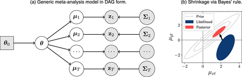
Notes. In the directed acyclic graph (DAG) in panel (a), circles denote random variables, and the box denotes a fixed a priori value. Shading denotes values that are observed or known. We assume with for all . The vector denotes fixed hyperparameters for the prior distribution on . The plot in panel (b) provides an example in which Bayesian shrinkage significantly improves the point estimate, , and its variance because of the strong prior correlation between and . (a) Generic meta-analysis model in DAG form. (b) Shrinkage via Bayes’ rule.
3.4. Extension to Metaregression
Given experiment-level metadata—target platform, intervention type, test duration, etc.—Assumption 4 can be relaxed to allow the distribution of to vary by test, resulting in a metaregression model (van Houwelingen et al. 2002). Mathematically, this information can be encoded in a covariate vector for some . Assumption 4 can then be relaxed to require only conditional independence across tests given and ; in the assumption below, represents a generic value of and means “independently distributed as.”
(
The vector can also include summaries of ; this may be required if especially high- or low-performing tests are stopped quickly, resulting in large variances. Analysts may also include time variables in to capture changes in the effect distribution over time. In general, we recommend using model checking to determine whether a metaregression model is needed and if so, which variables to include in .
The data in our empirical study do not contain rich experiment-level metadata, and we find limited evidence of dependence between and . Consequently, with the exception of the simulation study in Section 5, the remainder of the paper focuses on meta-analytic models under Assumption 4. The next section presents three representative models in this context.5
4. Meta-Analysis Models
Having outlined the basic meta-analysis framework, we now provide three specific meta-analysis models that we compare in Sections 5 and 6.
4.1. Multivariate Gaussian Model
We first consider a multivariate Gaussian model for : , where and with . Given and (or posterior samples thereof), it is well known that the posterior distribution of is available in closed form:
A particularly desirable feature of the BLUPs is that they represent a linear combination of and , which can aid in interpretation. Further, in a standard asymptotic regime with , we have and as . Thus, the BLUP is asymptotically equivalent to the naive estimator, , and produces the same asymptotic inferences. In finite samples, however, the BLUP can substantially outperform the naive estimator, especially when is highly concentrated—a common scenario in online experimentation.
BLUPs generalize naturally to the setting in which is only partially observed provided that the missingness is not systematic.6 In this case, the observed effect estimates can be written in the form for some matrix ; for example, if the first elements of are not observed, we set , where is an identity matrix of dimension . The analysis is then modified by replacing the term in (4) with and modifying the estimation algorithm accordingly. For the Gaussian model, this modification results in the following posterior parameters in place of those given in (5):
If is missing, for example, the term is equal to : the (invertible) submatrix of corresponding to . The implication for the OEC meta-analysis framework is that we can obtain inferences for unobserved metrics—including long-term metrics before their time frame has elapsed—provided that we have access to short-term proxies. Notably, this approach does not require restrictive causal assumptions beyond what is needed for standard effect estimation. Rather, it requires that and are correlated; these correlations are encoded in , and stronger correlations result in more precise inference for . The Student-t and DPM models can be modified in a similar fashion to allow for missing data.
In practice, is unknown and must be estimated, so posterior summaries for and effectively average over the BLUPs defined in (5) according to the posterior density associated with different values of . Depending on the choice of computational approach, this posterior averaging may occur implicitly. All three models that we consider admit efficient “collapsed” Gibbs samplers (Liu et al. 1994), so we employ this computational approach throughout, although other techniques, such as Hamiltonian Monte Carlo (HMC), could also be applied (Brooks et al. 2011, Neal 2011). The Gibbs sampling methods that we employ are well known (Neal 2000); however, to assist practitioners in applying our methods, we include them in Appendix B with specific suggestions on how to specify the hyperprior. In general, we recommend specifying dispersed, weakly informative prior distributions where possible, allowing the data set to “speak for itself” in terms of specifying plausible values for . For small T, this specification has the benefit of producing estimates that closely align with those of the naive method; as T increases, the estimates improve as the model develops a better estimate of .
Buyse et al. (2000) were the first to propose a (bivariate) version of this model in the surrogate end-points literature. Buyse et al. (2000) note that the strength of a surrogate can be assessed by the coefficient of determination from a regression of on : , where the indices denote elements of corresponding to either or . In the case of vector-valued , this measure generalizes naturally to . When is also vector valued and we employ the summed OEC of Example 2, we can further generalize this surrogacy measure as
For test t, we define the total variance ratio () as the ratio of the meta-analysis posterior variance to the naive variance: , where and with . This ratio can be interpreted in terms of cost savings as follows; achieving a similar posterior variance (or standard error) using the naive method would require increasing the sample size by a factor of . To further understand the source of the variance reduction, we define the intermediate quantity : the posterior variance from a hypothetical meta-analysis using only (discarding ). We can then define the prior variance ratio (PVR), , and surrogacy variance ratio (SVR), , representing the multiplicative effects on the posterior variance because of (i) the prior distribution of and (ii) surrogacy of for , respectively. Because the elements of may, in general, correlate with one another, includes reduction in the variance attributable to internal surrogacy: surrogacy of the elements of for one another.7
Having defined these quantities, we can then decompose as to assess the contribution of each component to the efficiency gain. These metrics can also be computed for the individual components of , providing measures of surrogacy for one outcome given all of the others—a strategy that we employ in our analysis in Section 6. In practice, we recommend using these surrogacy metrics to inform which metrics to include in so as to maximize the strength of surrogacy subject to model complexity constraints.
4.2. Multivariate Student-t Model
Previous work has noted that large outliers are empirically much more common in A/B testing than the Gaussian assumption of Section 4.1 would allow (Azevedo et al. 2020). Perhaps the simplest extension of Section 4.1 to capture this phenomenon is to allow to take the form of a multivariate Student-t distribution:
4.3. DPM Model
The Gaussian and Student-t models serve as a useful starting point, especially when A/B tests are believed to be fairly homogeneous. This section introduces the DPM method, a flexible nonparametric model that avoids placing restrictive parametric assumptions on . The DPM method assumes that are drawn from a mixture distribution, , where itself is a random draw from a Dirichlet process with base distribution and concentration parameter . Formally, the DPM model can be represented as
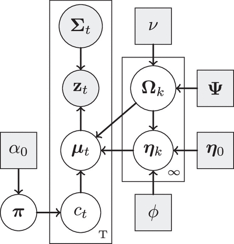
Notes. Shape type and shading denote whether the variable is random or observed, respectively, as in panel (a) of Figure 1. The grouping rectangles (plates) represent conditionally independent random variables, with the degree shown in the bottom right. In the case of and , the degree is infinite because the DPM model allows for an infinite number of latent clusters.
The surrogacy measures , TVR, PVR, and SVR generalize in a straightforward manner to the DPM model by replacing with the cluster-specific covariance matrices, , where is the estimated number of clusters. These measures can be used in a cluster-specific or test-specific manner or aggregated across tests and clusters to obtain integrated measures of surrogacy.
5. Simulation Study
We performed a simulation study to compare the performance of the methods developed in Section 4. The simulations comprise independent replicates with known ground-truth values, enabling a richer comparison than is possible in our empirical study in Section 6. In particular, the synthetic nature of the data allows us to compute a larger set of performance metrics and apply a metaregression model based on a synthetic cluster membership variable.
5.1. Simulation Setup
To enforce fidelity between the simulation study and data analysis, we draw 100 independent data sets from the DPM model’s posterior predictive distribution after fitting it to the observed data set as described in Section 6.1. However, we apply transformations, including translations, rescalings, and rotations, to ensure that the simulated data set does not reveal any material nonpublic information regarding Zillow’s business metrics or experimentation processes. We have made these simulated data sets available on the Open Science Framework to allow researchers to reproduce and build on our results. The simulation analyses use the same methods, prior distributions, and computational algorithms as the empirical analysis described in Section 6.
In addition to testing the three meta-analysis approaches introduced in Section 4, we also implement the naive plug-in method described in (1), which mimics the common industry practice of analyzing A/B tests individually with no shared prior distribution. All methods use the same values of and as input. We also include two additional variations of the methods presented in Section 4: Gaussian-0 (G-0) and metaregression. The Gaussian-0 model fixes , allowing us to quantify the benefit of estimating the prior metric mean compared with fixing it to zero. MR is a metaregression variant of the DPM model in which the cluster labels are known. From a practical standpoint, this represents a setting in which experiment type is known a priori—for example, mobile versus browser tests—so that the effect distribution may differ across known but related groups. For brevity, the method names are sometimes abbreviated N, G-0, G, T, DPM, and MR.
5.2. Simulation Results
We first compare the methods on six performance metrics.
Correct decision rate. The percentage of tests that correctly identify the test arm (A or B) that will maximize : B if and else, A.
Regret. The difference in between the selected arm and the optimal arm.
Overestimation. The average estimation error (predicted − true) for among selected arms. This metric quantifies the overstatement that arises when variants are selected for implementation or reporting because their estimated OEC is positive.
Mean absolute error (MAE). The average (across tests) absolute error in the estimation of .
Average 95% confidence interval (95% CI) length. The average (across tests) length of 95% credible (confidence) intervals for .
95% CI coverage. The coverage rate for the above 95% credible (confidence) intervals.
In the results reported below, we first compute these metrics within each replication, and then, we compute averages and standard errors across replications. Figure 3 displays the average values of the six metrics introduced above with 95% confidence intervals. To enhance the precision of the comparison, we also report the underlying metric values in Table 1.
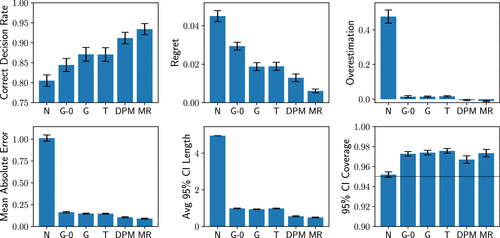
Notes. These bar charts visualize the simulation performance detailed in Table 1. The error bars represent 95% confidence intervals. The labels correspond to the naive, Gaussian-0, Gaussian, Student-t, Dirichlet process mixture, and metaregression methods, respectively.
|

Table 1. Simulation Results
| N | G-0 | G | T | DPM | MR | |
|---|---|---|---|---|---|---|
| Correct Decision Rate | 0.81 (0.01) | 0.84 (0.01) | 0.87 (0.01) | 0.87 (0.01) | 0.91 (0.01) | 0.93 (0.01) |
| Regret | 0.05 (0.00) | 0.03 (0.00) | 0.02 (0.00) | 0.02 (0.00) | 0.01 (0.00) | 0.01 (0.00) |
| Overestimation | 0.48 (0.02) | 0.01 (0.00) | 0.01 (0.00) | 0.02 (0.00) | −0.01 (0.00) | −0.01 (0.00) |
| MAE | 1.01 (0.02) | 0.16 (0.00) | 0.15 (0.00) | 0.15 (0.00) | 0.11 (0.00) | 0.09 (0.00) |
| Avg 95% CI Length | 4.95 (0.00) | 0.98 (0.01) | 0.94 (0.01) | 0.98 (0.01) | 0.56 (0.01) | 0.49 (0.01) |
| 95% CI Coverage | 0.95 (0.00) | 0.97 (0.00) | 0.97 (0.00) | 0.98 (0.00) | 0.97 (0.00) | 0.97 (0.00) |
Notes. Performances of the six methods in the simulation study across six performance metrics (standard errors) are shown. The column headings correspond to the naive, Gaussian-0, Gaussian, Student-t, Dirichlet process mixture, and metaregression methods, respectively. See Figure 3 for a visualization of these values. Avg, average; MAE, mean absolute error.
In the upper left panel of Figure 3, we see that the meta-analysis methods correctly identify the winning variant more frequently than the naive method, resulting in lower regret in the upper center panel of Figure 3. In both comparisons, the Gaussian and Student-t methods perform similarly, correctly identifying the winning arm in 87% of tests compared with 81% for the naive method, 84% for the Gaussian-0 method, 91% for the DPM method, and 93% for the metaregression method. Thus, compared with the naive method, the DPM and metaregression methods reduce the number of incorrect decisions by more than 50%. The upper right panel of Figure 3 shows that the naive method substantially overestimates the effects of implemented variants, where implementation is based on positive estimated effects, with an average overestimation of 0.48 compared with negligible values in the range of [−0.01 to 0.02] for the meta-analysis methods.
The lower left panel of Figure 3 shows that the MAE follows a pattern similar to that of the above metrics; the metric improves (decreases) from left to right, with the DPM and MR methods performing best. The remaining lower center and lower right panels of Figure 3 compare the 95% credible (confidence) intervals. The meta-analysis methods produce intervals less than one fifth the length of the naive intervals (on average), yet they also cover at a higher rate. As expected, the naive method has near-nominal coverage of 95.2%. In contrast, the meta-analysis methods exhibit mild overcoverage—a consequence of employing misspecified (hyper-)prior distributions.8 The DPM and MR methods produce the narrowest intervals, presumably because their assumed prior distribution matches the data-generating process, enabling these methods to accurately adjust credible regions based on cluster membership.
Table 2 displays pair-wise comparisons across five9 of the six metrics listed above and two additional metrics: the Win Rate and the Mean log Error Quotient (MLEQ). The Win Rate is defined as the percentage of A/B tests in which the method listed in the row outperformed the method listed in the column in terms of the magnitude of estimation error. The MLEQ is defined as , where a is the row prediction, b is the column prediction, and c is the ground-truth value of ; more negative MLEQ indicates that the row method has smaller error. The meta-analysis methods outperform the naive method across both the Win Rate and MLEQ metrics, and the performance ordering is MR, DPM, T, Gaussian, Gaussian-0, and naive from best to worst. The MR and DPM methods outperform each of the other four methods at least 67% of the time (in separate comparisons). The performance order is consistent across the remaining performance metrics (excluding the 95% CI coverage, which is at or above the nominal 95% level for all methods). In total, 98 of 105 pair-wise comparisons are statistically significant, with all 7 nonsignificant comparisons involving the Gaussian-0, Gaussian, and T methods.
|
Table 2. Simulation Pair-Wise Method Comparisons
| Metric | Method | N | G-0 | G | T | DPM | MR |
|---|---|---|---|---|---|---|---|
| Win Rate | N | — | 0.25 (0.01) | 0.23 (0.01) | 0.22 (0.01) | 0.21 (0.00) | 0.20 (0.00) |
| G-0 | 0.75 (0.01) | — | 0.44 (0.01) | 0.42 (0.01) | 0.30 (0.01) | 0.27 (0.00) | |
| G | 0.77 (0.01) | 0.56 (0.01) | — | 0.45 (0.01) | 0.33 (0.01) | 0.30 (0.01) | |
| T | 0.78 (0.01) | 0.58 (0.01) | 0.55 (0.01) | — | 0.33 (0.01) | 0.30 (0.01) | |
| DPM | 0.79 (0.00) | 0.70 (0.01) | 0.67 (0.01) | 0.67 (0.01) | — | 0.42 (0.01) | |
| MR | 0.80 (0.00) | 0.73 (0.00) | 0.70 (0.01) | 0.70 (0.01) | 0.58 (0.01) | — | |
| Mean log Error Quotient | N | — | 0.63 (0.02) | 0.71 (0.02) | 0.72 (0.02) | 1.12 (0.03) | 1.23 (0.03) |
| G-0 | −0.63 (0.02) | — | 0.08 (0.01) | 0.09 (0.01) | 0.50 (0.02) | 0.60 (0.02) | |
| G | −0.71 (0.02) | −0.08 (0.01) | — | 0.01 (0.01) | 0.41 (0.02) | 0.52 (0.02) | |
| T | −0.72 (0.02) | −0.09 (0.01) | −0.01 (0.01) | — | 0.41 (0.02) | 0.51 (0.02) | |
| DPM | −1.12 (0.03) | −0.50 (0.02) | −0.41 (0.02) | −0.41 (0.02) | — | 0.11 (0.01) | |
| MR | −1.23 (0.03) | −0.60 (0.02) | −0.52 (0.02) | −0.51 (0.02) | −0.11 (0.01) | — | |
| Correct Decision Rate | N | — | −0.04 (0.00) | −0.07 (0.00) | −0.07 (0.00) | −0.11 (0.01) | −0.13 (0.01) |
| G-0 | 0.04 (0.00) | — | −0.03 (0.00) | −0.03 (0.00) | −0.07 (0.01) | −0.09 (0.01) | |
| G | 0.07 (0.00) | 0.03 (0.00) | — | 0.00 (0.00) | −0.04 (0.00) | −0.06 (0.01) | |
| T | 0.07 (0.00) | 0.03 (0.00) | −0.00 (0.00) | — | −0.04 (0.00) | −0.06 (0.00) | |
| DPM | 0.11 (0.01) | 0.07 (0.01) | 0.04 (0.00) | 0.04 (0.00) | — | −0.02 (0.00) | |
| MR | 0.13 (0.01) | 0.09 (0.01) | 0.06 (0.01) | 0.06 (0.00) | 0.02 (0.00) | — | |
| Regret | N | — | 0.02 (0.00) | 0.03 (0.00) | 0.03 (0.00) | 0.03 (0.00) | 0.04 (0.00) |
| G-0 | −0.02 (0.00) | — | 0.01 (0.00) | 0.01 (0.00) | 0.02 (0.00) | 0.02 (0.00) | |
| G | −0.03 (0.00) | −0.01 (0.00) | — | −0.00 (0.00) | 0.01 (0.00) | 0.01 (0.00) | |
| T | −0.03 (0.00) | −0.01 (0.00) | 0.00 (0.00) | — | 0.01 (0.00) | 0.01 (0.00) | |
| DPM | −0.03 (0.00) | −0.02 (0.00) | −0.01 (0.00) | −0.01 (0.00) | — | 0.01 (0.00) | |
| MR | −0.04 (0.00) | −0.02 (0.00) | −0.01 (0.00) | −0.01 (0.00) | −0.01 (0.00) | — | |
| Overestimation | N | — | 0.46 (0.02) | 0.46 (0.02) | 0.46 (0.02) | 0.48 (0.02) | 0.49 (0.02) |
| G-0 | −0.46 (0.02) | — | −0.00 (0.00) | −0.00 (0.00) | 0.02 (0.00) | 0.03 (0.00) | |
| G | −0.46 (0.02) | 0.00 (0.00) | — | −0.00 (0.00) | 0.02 (0.00) | 0.03 (0.00) | |
| T | −0.46 (0.02) | 0.00 (0.00) | 0.00 (0.00) | — | 0.02 (0.00) | 0.03 (0.00) | |
| DPM | −0.48 (0.02) | −0.02 (0.00) | −0.02 (0.00) | −0.02 (0.00) | — | 0.01 (0.00) | |
| MR | −0.49 (0.02) | −0.03 (0.00) | −0.03 (0.00) | −0.03 (0.00) | −0.01 (0.00) | — | |
| MAE | N | — | 0.85 (0.02) | 0.87 (0.02) | 0.87 (0.02) | 0.91 (0.02) | 0.92 (0.02) |
| G-0 | −0.85 (0.02) | — | 0.02 (0.00) | 0.02 (0.00) | 0.06 (0.00) | 0.07 (0.00) | |
| G | −0.87 (0.02) | −0.02 (0.00) | — | 0.00 (0.00) | 0.04 (0.00) | 0.06 (0.00) | |
| T | −0.87 (0.02) | −0.02 (0.00) | −0.00 (0.00) | — | 0.04 (0.00) | 0.06 (0.00) | |
| DPM | −0.91 (0.02) | −0.06 (0.00) | −0.04 (0.00) | −0.04 (0.00) | — | 0.02 (0.00) | |
| MR | −0.92 (0.02) | −0.07 (0.00) | −0.06 (0.00) | −0.06 (0.00) | −0.02 (0.00) | — | |
| Avg 95% CI Length | N | — | 3.97 (0.01) | 4.01 (0.01) | 3.97 (0.01) | 4.39 (0.01) | 4.46 (0.01) |
| G-0 | −3.97 (0.01) | — | 0.05 (0.01) | 0.00 (0.01) | 0.43 (0.01) | 0.50 (0.01) | |
| G | −4.01 (0.01) | −0.05 (0.01) | — | −0.04 (0.01) | 0.38 (0.01) | 0.45 (0.01) | |
| T | −3.97 (0.01) | −0.00 (0.01) | 0.04 (0.01) | — | 0.43 (0.01) | 0.49 (0.01) | |
| DPM | −4.39 (0.01) | −0.43 (0.01) | −0.38 (0.01) | −0.43 (0.01) | — | 0.07 (0.01) | |
| MR | −4.46 (0.01) | −0.50 (0.01) | −0.45 (0.01) | −0.49 (0.01) | −0.07 (0.01) | — |
Notes. Numeric values denote comparisons between the row method and the column method (row – column for the metrics prefixed by ). Except for the Win Rate section, positive (negative) values represent comparisons in which the metric value for the row (column) exceeded that of the column (row). The values in parentheses denote the estimated standard error for these comparisons. The abbreviations in the column headings correspond to the naive, Gaussian-0, Gaussian, Student-t, Dirichlet process mixture, and metaregression methods, respectively. Avg, average; MAE, mean absolute error.
In summary, the meta-analysis methods substantially outperform the naive method. The Gaussian and T methods perform comparably with each other and slightly better than the Gaussian-0 method. The DPM and MR methods substantially outperform the other methods. Of these two methods, the MR method performs best, presumably because it has access to the cluster membership variables, which the DPM method must estimate.
6. Application to Real Estate Technology A/B Tests
In this section, we present results from applying the Bayesian meta-analysis methods to 190 A/B tests from Zillow. These tests represent all A/B tests during a subset of 2022–2024 that meet certain data quality standards, such as involving a sufficiently large number of users and not exhibiting unexpected imbalances in the assignment proportions. The A/B tests involve a variety of interventions ranging from new or altered email campaigns to website design changes, new product features, and updated personalization models. For each A/B test, we use the largest available sample (i.e., the most mature cohort). In most cases, these samples correspond with the data that were used to make implementation decisions.
6.1. Analysis Setup
Zillow receives revenue through various interrelated lines of business: new construction, rentals, sales leads for real estate agents, mortgages, products for sellers (e.g., promoted homes), and more. We might reasonably expect some lines of business to operate synergistically and others to result in cannibalization. To maintain confidentiality, we restrict attention to only two (undisclosed) lines of business, specifying as estimates of the (rescaled) financial impact of the tested interventions on each individual line of business in terms of dollars per customer. If, for example, the two lines of business were new construction and rentals, would consist of two components, and , representing the estimated per-customer effect of experiment t on revenue for new construction and rentals, respectively. Consequently, the natural definition for in this case is —the sum over the two lines of business as in Example 2.
The vector consists of three short-term proxies for . Although we cannot disclose the specific definitions of these proxies, typical proxy metrics in this industry include measures of customer engagement, form-fill rates, and shorter-horizon measurements of . The primary purpose of including these proxies is to increase the model’s posterior precision by including causal effect estimates that are predictive of as quantified by the surrogacy measures given in Section 4.1.
We implemented all meta-analysis methods in Python using the collapsed Gibbs samplers described in Appendix B. For the priors, we set , , , and for the Gaussian and T methods. For the T method, we assumed the prior with a prior median of degrees of freedom. For the DPM, we set hyperpriors as follows: , , , , and . Appendix C details a sensitivity analysis showing that the results in Section 6.2 are quite robust to specification of the prior distribution. We drew 30,000 samples for each method, with the first 10,000 samples discarded as warm-up iterations. The computation times were 1.35, 2.45, 4.73, and 142.53 minutes for the Gaussian-0, Gaussian, T, and DPM methods, respectively, on a cloud server with eight central processing units (CPUs) and 32 GB of memory. Appendix B.4 provides additional details on the computational scalability of our methods.
6.2. Sample-Split Predictive Analysis
To evaluate the methods’ performance, we implement a sample-splitting approach, in which each A/B test is randomly divided at the customer level into two equal-sized subsets: a training set and a test set. We fit the methods on the training set, obtaining posterior-based estimates of . We then compare these estimates with independent estimates generated from the test set. We generate these estimates using , the naive estimator, because the naive method is asymptotically unbiased under only Assumptions 1 and 3; in particular, it does not require a correctly specified parametric model or even i.i.d. effects (Assumption 4). Consequently, it serves as an independent holdout benchmark for predictive evaluation in the empirical setting. In addition to point estimates, we produce 95% posterior predictive intervals for the naive test-set estimates of for each method. These intervals allow us to assess whether the inferences from the meta-analysis methods are appropriately calibrated.
Table 3 summarizes the methods’ predictive performance in terms of two performance metrics defined in Section 5.2: the Win Rate and MLEQ. The definitions of these metrics are modified slightly to accommodate the fact that we no longer have access to the ground-truth values of ; we replace these ground-truth values with the naive method’s test-set estimates. We see that the four meta-analysis methods substantially outperform the naive approach in terms of the Win Rate, achieving lower prediction error in 69%–73% of A/B tests. The MLEQ metric produces the same conclusion as the Win Rate—that the meta-analysis methods substantially outperform the naive method. Among the meta-analysis methods, DPM and T perform best overall, with Gaussian and Gaussian-0 performing similarly but clearly better than the naive method. The DPM-naive comparison in the MLEQ block equals , meaning that the DPM’s log absolute prediction error is 0.29 points lower than that of the naive method. Because this comparison is on the log absolute-error scale, exponentiating gives ; equivalently, the DPM method reduces absolute prediction error by about 25% on the original scale. Quantifying the uncertainty in these performance metrics is challenging because the meta-analysis predictions are statistically dependent. The standard errors shown in parentheses in Table 3 are calculated assuming independence of the predictions, so they should be interpreted as rough approximations. We address the uncertainty quantification more rigorously in our simulation study in Section 5 using independent replications. Compared with the results in Table 2, we see that the predictive nature of this comparison dilutes the differences between methods because (i) the “true value” in this analysis is a noisy estimate of and (ii) the estimates are formed using only 50% of the data.
|
Table 3. Pair-Wise Method Comparisons for Predictive Performance
| Metric | Method | Naive | Gaussian-0 | Gaussian | T | DPM |
|---|---|---|---|---|---|---|
| Win Rate | Naive | — | 0.27 (0.03) | 0.27 (0.03) | 0.28 (0.03) | 0.31 (0.03) |
| Gaussian-0 | 0.73 (0.03) | — | 0.55 (0.04) | 0.39 (0.04) | 0.43 (0.04) | |
| Gaussian | 0.73 (0.03) | 0.45 (0.04) | — | 0.40 (0.04) | 0.43 (0.04) | |
| T | 0.72 (0.03) | 0.61 (0.04) | 0.61 (0.04) | — | 0.41 (0.04) | |
| DPM | 0.69 (0.03) | 0.57 (0.04) | 0.57 (0.04) | 0.59 (0.04) | — | |
| Mean log Error Quotient | Naive | — | 0.22 (0.07) | 0.22 (0.07) | 0.28 (0.08) | 0.29 (0.08) |
| Gaussian-0 | −0.21 (0.07) | — | 0.00 (0.01) | 0.06 (0.04) | 0.08 (0.06) | |
| Gaussian | −0.22 (0.07) | 0.00 (0.01) | — | 0.06 (0.04) | 0.08 (0.06) | |
| T | −0.27 (0.08) | −0.06 (0.04) | −0.06 (0.04) | — | 0.02 (0.07) | |
| DPM | −0.29 (0.08) | −0.08 (0.06) | −0.08 (0.06) | −0.02 (0.07) | — |
Notes. Pair-wise predictive performances of the five methods in the empirical application are shown with approximate standard errors in parentheses. The Win Rate section displays the proportion of tests in which the method listed in the row outperformed the method listed in the column. In the Mean log Error Quotient section, a negative (positive) value indicates that the row (column) method outperformed the column (row) method.
Figure 4 visually compares the methods’ absolute prediction errors in a pair-wise fashion. Below the diagonal in Figure 4, methods listed in each row can visually be seen to outperform the method listed in the column when the points fall below the line. These plots in Figure 4 provide visual confirmation of the relative performances shown in Table 3. In particular, we see that the meta-analysis methods typically produce smaller absolute prediction errors than the naive method. The large differences in scale can be observed by noting that the absolute prediction errors shown are plotted on the log scale, with most values falling between 0.01 and 100.
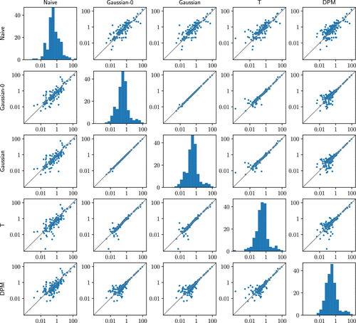
Notes. Each coordinate represents the absolute prediction error for the corresponding method in the empirical application. The diagonal lines represent exactly equal performance. The DPM’s prediction errors are the smallest, indicating that it produced the most accurate estimates of on average.
Figure 5 plots the ranks of the predictions against the ranks of the prediction errors. Ideally, we would see no linear relationship between these ranks, indicating that the inferences are unbiased in a conditional sense (i.e., given a subset of tests having estimated equal to , the conditional expectation of for these tests is, in fact, equal to the estimate, u). Although this seems to be a natural methodological requirement, the naive approach does not satisfy it because of regression to the mean. This shortcoming is visually apparent in panel (a) of Figure 5 with the strong negative correlation between the predictions and errors (). In common practice, A/B tests with large, statistically significant estimates are implemented and internally reported. The unfortunate implication is that the impact of these “winning” tests is typically overstated. Bayesian methods provide a natural fix for this problem by performing conditional inference; under correct model specification, the posterior mean possesses a conditional unbiasedness property by design. This property is evident in panels (b)–(e) of Figure 5, which show much lower correlation between prediction ranks and error ranks compared with the naive approach ( in all four cases). The DPM model achieves the greatest reduction as evidenced by the relatively flat line in panel (e) of Figure 5 and a small Spearman rank correlation of −0.14. This finding suggests that the DPM method is likely modeling the true prior distribution, , more accurately than the other methods. It effectively debiases the naive estimates () by accurately modeling the heterogeneity in the true effects () via its flexible representation of the prior distribution as a mixture of inferred clusters. It regularizes each estimate just enough that its expected error is near zero regardless of the value of the naive estimate. This property can also be seen in the overestimation metric in Section 5.2, which is almost exactly zero for the DPM method.

Notes. The large negative trend in panel (a) indicates regression to the mean. In contrast, the flatter regression lines and smaller absolute values of the Spearman correlation (Corr.) coefficient in the remaining panels indicate that the meta-analysis methods mitigate this phenomenon. The DPM method in panel (e) in particular shows the least evidence of regression to the mean among the fitted models. (a) Naive. (b) Gaussian-0. (c) Gaussian. (d) T. (e) DPM.
Table 4 compares the performance of the methods’ prediction intervals. All methods produce near-nominal coverage. However, the meta-analysis methods produce shorter intervals. This is especially true of the DPM method, which produces median interval lengths that are about 25% shorter than those of the naive method, indicating substantial benefit from including a prior distribution for the values. Again, the predictive nature of this comparison dilutes the difference in interval width.
|
Table 4. Performance of 95% Prediction Intervals
| N | G-0 | G | T | DPM | |
|---|---|---|---|---|---|
| Coverage | 0.95 | 0.94 | 0.95 | 0.96 | 0.96 |
| Median length | 2.06 | 1.78 | 1.78 | 1.83 | 1.55 |
| Mean length | 10.21 | 7.38 | 7.38 | 7.75 | 7.21 |
Notes. The 95% prediction interval coverage is shown for the methods tested in the empirical application: naive, Gaussian-0, Gaussian, Student-t, and Dirichlet process mixture. All methods achieve approximately nominal coverage. However, the meta-analysis methods produce much shorter prediction intervals on average.
6.3. Full-Data Analysis
In addition to the sample-split predictive analysis, we also applied the DPM method to the full data set. To evaluate Assumption 4, we used the DPM model to compute posterior predictive p-values, checking for correlation between the entries of (and their absolute values) and the corresponding variance entries in . The smallest posterior predictive p-value was 0.05. With 10 comparisons, this represents only minimal evidence against Assumption 4. The rest of the analysis provides insights into the inner workings of the DPM model and the latent structure of the causal effects across tests.
Table 5 displays estimates of the surrogacy measures introduced in Section 4.1. Because the DPM model produces test-specific estimates of these measures, we average their values across tests to obtain estimates of the overall strength of surrogacy. The estimated values of fall in the range from 0.46 to 0.78, indicating moderately strong surrogacy. Effects on the surrogates () do, in fact, predict effects on the KPIs (); however, they do so imperfectly. The value for is smaller than that of both and , indicating that and show some degree of internal surrogacy. The estimates of TVR are in the range from 0.10 to 0.16, indicating a reduction in the posterior standard deviation of over 60% compared with the naive approach. Achieving a comparable reduction using the naive method alone would require increasing the sample size by a factor of ; here, this corresponds with a factor of 6–10, which is not achievable because these tests are continuously run in sequence across different teams. These metrics can also be used to expand and refine the list of included surrogates. For instance, Table 5 indicates that the surrogates for have larger values than those for , suggesting that the analysis may benefit relatively more from adding a strong surrogate for compared with adding a strong surrogate for .
|
Table 5. Aggregate Surrogacy Measures
| R2 | 0.52 (0.18–0.90) | 0.78 (0.42–0.98) | 0.46 (0.13–0.81) |
| TVR | 0.16 (0.08–0.24) | 0.10 (0.04–0.19) | 0.15 (0.08–0.24) |
| PVR | 0.18 (0.10–0.27) | 0.13 (0.06–0.22) | 0.17 (0.10–0.26) |
| SVR | 0.91 (0.82–0.97) | 0.88 (0.79–0.95) | 0.93 (0.84–0.97) |
Notes. Posterior means for aggregated surrogacy measures from the DPM model (95% credible intervals) are shown. The surrogacy measures (defined in Sections 4.1 and 4.3) are averaged over all 190 tests. Notably, the low values of PVR relative to SVR indicate that in this application, most of the variance reduction arises from prior regularization of the long-run outcomes themselves, with the short-term proxies providing additional but comparatively smaller gains.
Figure 6 displays heat maps that visualize the inner workings of the DPM model. The posterior mean for the number of clusters is 7.2 with a 95% credible interval of 4–12. Panel (a) of Figure 6 plots posterior probabilities that pairs of tests are clustered together. These probabilities represent the model’s posterior belief that the tests arise from the same distribution. We used hierarchical clustering methods (Murtagh and Contreras 2012) to group and sort the tests.10 Doing so reveals the existence of several small, distinct clusters that are internally homogeneous but distinct from the other clusters. We applied the DPM method to an enlarged set of business metrics and obtained similar results, although with more distinct clusters. Upon inspecting these clusters, we found many cases where the DPM method had clustered tests involving a similar intervention or platform. For instance, one cluster of tests primarily affected the search experience for rental properties, and another involved only tests implemented on mobile devices. In practice, these model-based clusterings could be used to identify experiment-level metadata that could be used within a metaregression model.
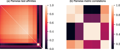
Notes. Panel (a) displays posterior probabilities that tests are clustered together (pair-wise affinities), revealing the existence of several small, distinct clusters. Panel (b) displays pair-wise estimated Pearson correlations for the latent effects () across experiments. Each location on the axis in panel (b) corresponds with one of the elements of ; the order of the metrics has been permuted to preserve confidentiality. (a) Pair-wise affinities. (b) Pair-wise metric correlations.
The values of and provide valuable strategic insights, such as the average effect of these interventions and how these effects correlate across metrics. An example of the latter is that the surrogacy relationships may differ across these clusters relative to the main cluster. The fact that the DPM model has access only to the values of and indicates that these groupings are apparent from the test results themselves. In addition to improving our estimates of , these latent groupings could be used to learn the “profile” of certain types of tests, which could be used to ideate and prioritize future interventions. In analyzing the tth test, the latent groupings could also inform decision making by comparing results across similar tests.
Panel (b) of Figure 6 displays estimated correlations among the components of . To further preserve confidentiality, the order of the metrics has been permuted. The plot in panel (b) of Figure 6 reveals that two pairs of metrics show strong positive correlation within pairs but are nearly uncorrelated between pairs. Additionally, the last metric shown is positively correlated with all four of the other metrics. The fact that all five metrics are, to varying degrees, positively correlated suggests that these metrics tend to have synergistic effects—improvements in one metric are associated with improvements in the others. Thus, in addition to offering improved effect estimates, the meta-analysis methods also uncover interpretable insights regarding the distribution of causal effects. As an example, suppose we learn that the treatment effects on a form-fill metric and a conversion metric are highly correlated across experiments. This finding implies that interventions improving the form-fill rate also tend to improve downstream conversions, which may influence the firm’s allocation of experimentation resources.
In the biostatistics literature on clinical trials, correlations like these are sometimes used to justify using one surrogate metric in place of another that is noisier or more difficult to measure. Although this strategy could be applied in A/B testing as well, we generally recommend selecting a target estimand () that closely aligns with long-term business goals and applying our meta-analysis methods to frame all subsequent inferences in terms of this estimand; the resulting strategy is analogous to the procedures proposed in Elliott et al. (2015) to avoid the so-called “surrogacy paradox,” in which a strong surrogate produces incorrect inferences for a particular intervention. A key benefit of the experimental meta-analysis approach over purely observational (e.g., data-mining) methods is that the effects are causal by design—not a misleading artifact of noncausal associations. Thus, in addition to improving A/B test decision making, the meta-analysis framework can provide crucial business insights that may be missed or badly biased in an observational analysis.
7. Discussion
This section provides a brief summary of our proposed framework, the relevant managerial considerations, and possible extensions.
7.1. Methodological and Results Summary
The primary contribution of this work is a meta-analytic framework for estimating the long-term value of A/B tests that (i) replaces additional causal surrogacy assumptions with an assumption that comparable experiments have exchangeable causal-effect vectors, (ii) leverages cross-metric relationships for increased efficiency, and (iii) is computationally scalable because of its reliance on summary statistics. Additionally, we demonstrate via simulation and an empirical application to 190 A/B tests in real estate technology that the proposed framework provides a large improvement over single-test analyses. Although our application is in real estate technology specifically, the framework is generally applicable to settings with many experiments that (i) share metric definitions, (ii) present little or no cross-experiment interference, and (iii) arise from a common domain so that the shared-effect distribution assumption in Assumption 4 or its conditional version in Assumption 5 is credible. Conversely, the framework is less suitable when experiments interfere significantly or differ sharply in domain, customer population, or metric definition unless these differences can be modeled explicitly through metaregression or careful filtering of the experiment archive.
We have presented three basic meta-analytic models: Gaussian, T, and DPM. We recommend informing the choice of the meta-analytic model via modeling diagnostics, including posterior model checking and information criteria (Spiegelhalter et al. 2002, Watanabe 2010). Because of its flexibility, we generally expect the DPM to outperform the Gaussian and T models; however, the latter two models can be fit much more quickly. In practice, analysts also have the flexibility to generalize well beyond these models, specifying metaregression models that allow the effect distribution to vary based on experiment attributes. When relevant sources of heterogeneity are omitted (e.g., differences in customer segments, product types, or experimental contexts), the model may be well calibrated only on average across experiments and can perform poorly for specific subsets of tests. In general, we expect that more heterogeneous experiments will require more flexible models to satisfy Assumption 4 or Assumption 5. Appendix A discusses additional practical considerations for applying our framework.
7.2. Managerial Implications
This work carries two primary managerial implications. First, Sections 5 and 6 uncovered a large statistical benefit in adopting meta-analytic methods. Our proposed framework offers a satisfying solution to the dilemma of choosing which business metrics or portion of the business funnel (top versus middle versus bottom) to prioritize. Our framework enables managers to define success in terms of bottom-of-funnel results (purchases, customer retention, etc.) and simultaneously reap the statistical benefits of top-of-funnel proxies (click-through rates, form-fill rates, etc.). These proxy metrics are relevant to decision making to the extent that causal effects on the proxies correlate with causal effects on strategic bottom-of-funnel outcomes. As a result, our meta-analysis methods provide a data-driven alternative to the industry practice of “OEC by committee,” in which business leaders manually select a set of metrics to prioritize. The meta-analysis methods also provide an elegant solution to the challenges of simpler OEC methods, including (i) the need to customize the OEC to different lines of business or software platforms, (ii) the inability to measure certain metrics for some tests because of technical constraints, and (iii) the sensitivity of the OEC definition to the time frame over which metrics are measured.
Second, our framework enables rigorous tracking of cumulative long-term experimental impacts, even when tests are selected for implementation or reporting based on large positive estimated effects. Because of the statistical phenomenon of regression to the mean, this common decision-making practice can substantially overstate cumulative impacts; see panel (a) of Figure 5 and our results on the overestimation metric in Section 5. Our meta-analytic framework addresses this problem by “shrinking” estimates toward regions of high prior probability, substantially reducing regression to the mean effects and the overstatement induced by selecting tests with large positive naive estimates . In practice, this feature of our framework can facilitate decision making surrounding organizational resource allocation and strategic priorities by producing reliable estimates of the financial value of implemented A/B tests.
7.3. Extensions
We present three common meta-analysis methods ranging from simple parametric models to flexible nonparametric alternatives. However, the statistical literature on meta-analysis and random-effects models is vast and includes many alternatives that could be applied within our OEC framework, including parametric and nonparametric empirical Bayes methods (Higgins et al. 2009, Efron 2014, Koenker and Mizera 2014). The Bayesian solutions presented here are notable for their extensibility and ability to provide actionable inferences, including surrogacy measures, explicit estimates of , and estimated clusterings.
Another promising direction is to develop methods that extrapolate effects beyond a short-term treatment window. Our framework can estimate the long-term impact of short-term treatments, averaging over any trends or business decisions between the test end date and the end of the measurement period. However, in some business settings, the true goal may be to estimate the long-term impact of long-term treatments, such as the effect on 12-month revenue of adding (versus not adding) a new feature over a 6-month period. This extension requires a different set of methods that effectively forecast the long-term effects using short-term proxies (Huang et al. 2026). Future work could consider how to combine these methods with the meta-analysis perspective presented here.
The authors thank Eric Ringger, Ryan Williamson, and other members of the data science and artificial intelligence organizations at Zillow for their important contributions to this research. The authors also thank the anonymous reviewers, the associate editor, and the senior editor for providing invaluable feedback that greatly improved the manuscript. Stephanie A. Nail, Terran Melconian, and Xan Vongsathorn are full-time employees at Zillow. Easton Huch was employed as an applied scientist intern while contributing to this study. Zillow has complete rights to review and require changes to this paper for any material objectionable to its interests, including the removal of intellectual property and trade secrets.
Appendix A. Additional Practical Considerations
In practice, tests with more than two arms are common. To accommodate these tests, we recommend stacking the effect estimates for the noncontrol arms into a single vector: , where is the total number of noncontrol arms and is the vector of effect estimates for the jth such arm. Similarly, the joint covariance matrix of these effect estimates can be formed as
The remaining Gibbs updates can be generalized in much the same fashion.
Another common practical challenge is that certain metrics may be missing because of (i) an incomplete measurement period or (ii) the inability to track certain outcomes in specific types of tests. In these cases, the Gibbs samplers can be modified as described in (6) and Appendix B. A simple (albeit less elegant) alternative is to fill the missing submatrix of with a large diagonal matrix and set the missing elements of to zero.
Operationally, we recommend maintaining a centralized archive of experiment-level summaries with standardized metric definitions and time windows, running periodic model checks, and adopting more flexible methods (nonparametric models and/or metaregression) when model assumptions are not satisfied. Teams can refit these models regularly (e.g., daily) using the most up-to-date estimates available, extracting posterior summaries of for in-progress tests. This process can be complemented by comparing early estimates with “mature estimates” available after all metrics are observed.
Appendix B. Gibbs Sampling Algorithms
This section provides the Gibbs samplers for the Gaussian, Student-t, and DPM models.
B.1. Gaussian Gibbs Sampler
For simplicity, we assume independent Gaussian and inverse-Wishart priors for and , respectively. Denoting the prior scale matrix and degrees of freedom as and , respectively, the complete conditional for is , where denotes an inverse-Wishart distribution and the posterior parameters are
We denote the prior mean and prior variance of as and , respectively. The parameters and can be blocked together in the Gibbs sampler by first integrating out the to improve mixing, resulting in a “collapsed” Gibbs sampler (Liu et al. 1994). The marginalized complete conditional distribution for is with posterior parameters
Similar to (6), we can handle partial observations by replacing with . After sampling , can then be sampled according to (5). Algorithm B.1 summarizes the Gibbs sampler.
In specifying the hyperprior, we recommend setting , corresponding to a prior belief that the average effect is zero. Because is well identified from the data, we recommend setting to a diagonal matrix with large nonzero entries. The prior for can likewise be set in a weakly informative fashion, selecting a small value of (such as p) and a corresponding value of that results in a prior mode that roughly matches a priori beliefs regarding the magnitude of the true effects ().
(
Input:
Sample from with defined in (B.1).
Sample from with defined in (B.2).
for do
Sample from with defined in (5b).
end for
B.2. Student-t Gibbs Sampler
Unlike the Gaussian model, the multivariate Student-t model is not conjugate given . However, it is conditionally conjugate if we introduce latent variables as follows:
This approach is a form of Bayesian data augmentation (Tanner and Wong 1987, van Dyk and Meng 2001). It maintains the assumption of (8) and introduces simple conditionally conjugate updates for and . The Gibbs sampler of Appendix B.1 can be extended to fit this model by introducing a sampling block for and . We recommend first integrating out and using a Metropolis–Hastings step to sample . Conditional on , the latent variables can then be sampled as , where denotes a gamma distribution and the rate parameter is . The remaining Gibbs blocks are similar to those in Appendix B.1 with the following rescalings by the ratio :
The posterior parameters and are adapted in a similar fashion, replacing with . As with the multivariate Gaussian model, the Gibbs steps can easily be generalized to the setting in which only is observed.
We recommend setting the hyperparameters , , , and as described in Appendix B.1. We recommend specifying a prior for such that it includes values ranging from high kurtosis () to nearly Gaussian () with high prior probability.
B.3. DPM Gibbs Sampler
Gibbs sampling is a particularly common computational approach for DPM models because their infinite parameter space and multimodality make them less amenable to HMC. We fit our DPM model via a collapsed Gibbs sampler (Neal 2000, algorithm 3). The sampler iteratively updates the cluster assignments, , based on the posterior predictive density of each cluster, , available in closed form as the following multivariate Student-t density:
The Gibbs sampler reassigns points to existing clusters with probabilities proportional to and to a new cluster with probability proportional to . This loop is the most computationally costly portion of the Gibbs sampler, but it can be optimized by updating the parameters in (B.4) via efficient rank-1 updates. After updating all in this manner, we sample from using the full set . We then update with a collapsed Gibbs step with the parameters modified from (B.2) as follows:
Subsequently, we update according to (5), replacing and with the cluster-specific parameters and , respectively. As with the multivariate Gaussian and Student-t methods, these steps can easily be adapted to the setting in which only is observed via slight modifications to the updates for , , and . The GEM parameter, , can be updated via Metropolis–Hastings or the conditionally conjugate data augmentation strategy given in Escobar and West (1995). The prior parameters , , , and can also be updated using conditionally conjugate priors or a Metropolis–Hastings step. Algorithm B.2 summarizes the full Gibbs scan.
(
Input:
for all
for do
Remove t from
if then
for all with
end if
Sample a new value for using g as defined in (B.3) with :
and append to
end for
Sample from with defined in (B.4)
Sample from with defined in (B.5)
Sample according to (5), substituting for and for
(Optional) Sample via Metropolis–Hastings or the data augmentation method given in Escobar and West (1995)
(Optional) Sample via conditionally conjugate distributions or Metropolis–Hastings
We recommend setting or estimating it with a prior centered in the same interval. Whenever feasible, we recommend specifying priors for , , , and . The prior for and can be set as explained in Appendix B.1. We recommend setting the prior for to a dispersed distribution on that includes the value of one, such as . We recommend setting the prior for to a dispersed multivariate Gaussian distribution centered at , similar to the above recommendation for setting and in the Gaussian and T methods.
B.4. Computational Scalability
With the cost of cloud CPU hours below $0.05, the computation time required for our methods represents a trivial cost for most technology firms. We generally expect the cost of computing and to be much higher than the cost of fitting these models. However, standard univariate A/B testing procedures already require computation of and , so the only additional required computations are the covariance terms (the off-diagonal elements) of .
The samplers scale approximately linearly in T, so the methods could easily scale to thousands of tests, especially the Gaussian and T methods, which can be parallelized across tests. The number of clusters, K, increases like (Rodriguez and Müller 2013, p. 27), so the DPM sampler scales like in the number of tests. The DPM sampler cannot be fully parallelized, but our approach could be optimized via implementation in a low-level language. It could also be split into multiple MCMC chains to reduce the required length of each individual chain. Previous model fits could also be used to “warm start” the sampler, removing the need for a long warm-up period.
Because the samplers involve matrix inversions, they scale as in the number of metrics. Consequently, including a large number of business metrics (say, ) could prove computationally prohibitive in the absence of programming optimizations. In most cases, we believe that our framework could be successfully applied to settings with , especially if researchers use the surrogacy measures of Section 4.1 to remove low-quality proxy metrics. Consequently, adjustments to the computational approach are likely needed only in exceptional cases. If computation time is a concern, practitioners could leverage work on scalable Bayesian computational methods, such as variational inference (Blei and Jordan 2006) or distributed MCMC (Bumbaca et al. 2020).
When applied in practice, the meta-analysis methods use a large database of previous experiments to generate inferences for a much smaller set of executing experiments. Thus, one simple strategy to reduce computational demands is to refit the meta-analysis method in batches (e.g., weekly) and apply the most-recent posterior samples of to generate estimates for currently running tests. This approach is only approximate in that it ignores recent data when estimating , but with a large number of previous experiments, the approximation is likely to be quite accurate. This batch estimation method is particularly straightforward for the Gaussian and T methods. It is also possible to apply it to the DPM method, although doing so would require a different model-fitting strategy that produces explicit estimates of .
Appendix C. Sensitivity Analysis
We performed a sensitivity analysis that mimics the sample-split analysis of Section 6.2, substituting a different prior distribution that meaningfully changes almost every hyperparameter. In particular, we set , , and for the Gaussian and T methods; we did not change the value of () because this is the most natural choice for this hyperparameter. For the T method, we assumed the prior with a prior median of degrees of freedom. For the DPM, we set hyperpriors as follows: , , , , and .
Employing this prior distribution resulted in only small changes to the results of Section 6.2. Table C.1 displays results analogous to Table 3 under this new prior distribution. The results indicate that the meta-analytic methods still substantially outperform the naive approach, and the performance ordering is similar to that of Table 3: DPM, T, Gaussian-0, Gaussian, and naive (from best to worst). None of the other results substantially alter any conclusions from Section 6.2. However, the lower prior mean for results in a smaller estimated number of clusters.
|
Table C.1. Pair-Wise Method Comparisons for Predictive Performance in Sensitivity Analysis
| Metric | Method | Naive | Gaussian-0 | Gaussian | T | DPM |
|---|---|---|---|---|---|---|
| Win Rate | Naive | — | 0.27 (0.03) | 0.29 (0.03) | 0.27 (0.03) | 0.32 (0.03) |
| Gaussian-0 | 0.73 (0.03) | — | 0.56 (0.04) | 0.31 (0.03) | 0.41 (0.04) | |
| Gaussian | 0.71 (0.03) | 0.44 (0.04) | — | 0.33 (0.03) | 0.41 (0.04) | |
| T | 0.73 (0.03) | 0.69 (0.03) | 0.67 (0.03) | — | 0.38 (0.04) | |
| DPM | 0.68 (0.03) | 0.60 (0.04) | 0.59 (0.04) | 0.62 (0.04) | — | |
| Mean log Error Quotient | Naive | — | 0.10 (0.05) | 0.09 (0.05) | 0.16 (0.06) | 0.30 (0.08) |
| Gaussian-0 | −0.10 (0.05) | — | 0.00 (0.00) | 0.07 (0.03) | 0.21 (0.07) | |
| Gaussian | −0.09 (0.05) | 0.00 (0.00) | — | 0.07 (0.03) | 0.21 (0.07) | |
| T | −0.16 (0.06) | −0.07 (0.03) | −0.07 (0.03) | — | 0.14 (0.06) | |
| DPM | −0.30 (0.08) | −0.21 (0.07) | −0.21 (0.07) | −0.14 (0.06) | — |
Notes. Pair-wise predictive performances of five methods on the sensitivity analyses are shown with approximate standard errors in parentheses; compare with Table 3. The Win Rate section displays the proportion of tests in which the method listed in the row outperformed the method listed in the column. In the Mean log Error Quotient section, a negative (positive) value indicates that the row (column) method outperformed the column (row) method.
1 Yang et al. (2024) show that this assumption can be relaxed somewhat to require only that the sign of the conditional average treatment effect (CATE) matches that of a surrogate-imputed CATE.
2 To be more precise, we could add an additional subscript to m to acknowledge that these outcomes are defined for individual customers. Our notation omits this dependence for brevity.
3 Rather than treating the analysis as a multivariate problem, practitioners often define one combined metric as a linear combination of individual metrics; this approach is easily seen to be equivalent to the naive approach owing to the linearity of both the estimator, , and the combined metric.
4 In Bayesian modeling, a hyperprior refers to a prior distribution for a prior distribution. The parameters of the hyperprior are often referred to as hyperparameters.
5 These could be extended to the metaregression setting by introducing a mixed-effects structure, such as , where is a mean-zero random effect and is a matrix of fixed-effect regression coefficients. A further generalization might allow the distribution of to depend on . These applied modeling techniques are largely context driven and have been used frequently in other areas of quantitative marketing; thus, we aim to provide only an introduction to the basic modeling techniques and leave the details of these generalizations to future applied work.
6 Specifically, Assumption 4 must continue to hold given missingness indicator variables. If the missingness is believed to be systematic, analysts can handle this challenge by specifying a metaregression model in which the distribution of depends on the missingness indicators.
7 In principle, the effect of internal surrogacy could be removed from by replacing with in the definition of , corresponding to an analysis in which we shrink the estimates toward their prior mean ignoring their prior correlations. Because this analysis is less natural than the analysis that simply discards , we have opted to define (and consequently, and ) using .
8 To make the simulation more realistic, we did not attempt to set prior parameters to closely match those of the data-generating process (from the fitted DPM model). In general, Bayesian methods do not deliver exact coverage under prior misspecification in finite samples.
9 We omit the differences in coverage rates because these differences all entail a standard error that rounds to 0.00.
10 Specifically, we used agglomerative clustering with complete linkage. We specified the distance metric as the posterior probability that a pair of tests belongs to different clusters.
References
- (2003) E-customization. J. Marketing Res. 40(2):131–145.Crossref, Google Scholar
- (2018) Retention futility: Targeting high-risk customers might be ineffective. J. Marketing Res. 55(1):80–98.Crossref, Google Scholar
- (2026) The surrogate index: Combining short-term proxies to estimate long-term treatment effects more rapidly and precisely. Rev. Econom. Stud. 93(4):2284–2312.Crossref, Google Scholar
- (2019) Empirical Bayes estimation of treatment effects with many A/B tests: An overview. AEA Papers Proc. 109:43–47.Crossref, Google Scholar
- (2020) A/B testing with fat tails. J. Political Econom. 128(12):4614–4672.Crossref, Google Scholar
- (1985) Statistical Decision Theory and Bayesian Analysis, Springer Series in Statistics, 2nd ed. (Springer-Verlag, New York).Crossref, Google Scholar
- (2018) Beyond the last touch: Attribution in online advertising. Marketing Sci. 37(5):771–792.Link, Google Scholar
- (2006) Variational inference for Dirichlet process mixtures. Bayesian Anal. 1(1):121–143.Crossref, Google Scholar
- (2011) Handbook of Markov Chain Monte Carlo (CRC Press, Boca Raton, FL).Crossref, Google Scholar
- (1973) Measurable selections of extrema. Ann. Statist. 1(5):902–912.Crossref, Google Scholar
- (2020) Scalable target marketing: Distributed Markov chain Monte Carlo for Bayesian hierarchical models. J. Marketing Res. 57(6):999–1018.Crossref, Google Scholar
- (2005) A Bayesian semiparametric model for random-effects meta-analysis. J. Amer. Statist. Assoc. 100(469):242–251.Crossref, Google Scholar
- (2000) The validation of surrogate endpoints in meta-analyses of randomized experiments. Biostatistics 1(1):49–67.Crossref, Google Scholar
- (2017) Links between causal effects and causal association for surrogacy evaluation in a Gaussian setting. Statist. Medicine 36(27):4243–4265.Crossref, Google Scholar
- (1954) The multivariate t-distribution associated with a set of normal sample deviates. Australian J. Phys. 7(4):531–542.Crossref, Google Scholar
- (2015) Objective Bayesian two sample hypothesis testing for online controlled experiments. Gangemi A, Leonardi S, Panconesi A (General Chairs), eds. Proc. 24th Internat. Conf. World Wide Web (Association for Computing Machinery, New York), 923–928.Google Scholar
- (2016) Data-driven metric development for online controlled experiments: Seven lessons learned. Krishnapuram B, Shah M (General Chairs), Smola A, Aggarwal C, Shen D, Rastogi R (Program Chairs), eds. Proc. 22nd ACM SIGKDD Internat. Conf. Knowledge Discovery Data Mining (Association for Computing Machinery, New York), 77–86.Google Scholar
- (2013) Improving the sensitivity of online controlled experiments by utilizing pre-experiment data. Leonardi S, Panconesi A (General Chairs), Ferragina P, Gionis A (Program Chairs), eds. Proc. Sixth ACM Internat. Conf. Web Search Data Mining (Association for Computing Machinery, New York), 123–132.Google Scholar
- (2023) From augmentation to decomposition: A new look at CUPED in 2023. Preprint, submitted December 5, https://doi.org/10.48550/arXiv.2312.02935.Google Scholar
- (1986) Meta-analysis in clinical trials. Controlled Clinical Trials 7(3):177–188.Crossref, Google Scholar
- (2015) Meta-analysis in clinical trials revisited. Contemporary Clinical Trials 45(Pt A):139–145.Crossref, Google Scholar
- (2018) Bayesian nonparametric customer base analysis with model-based visualizations. Marketing Sci. 37(2):216–235.Link, Google Scholar
- (2016) On the conditional distribution of the multivariate t distribution. Amer. Statistician 70(3):293–295.Crossref, Google Scholar
- (2014) Two modeling strategies for empirical Bayes estimation. Statist. Sci. 29(2):285–301.Crossref, Google Scholar
- (2023) Surrogate endpoints in clinical trials. Annual Rev. Statist. Appl. 10(1):75–96.Crossref, Google Scholar
- (2015) Surrogacy marker paradox measures in meta-analytic settings. Biostatistics 16(2):400–412.Crossref, Google Scholar
- (1995) Bayesian density estimation and inference using mixtures. J. Amer. Statist. Assoc. 90(430):577–588.Crossref, Google Scholar
- (2024) Causal machine learning for predicting treatment outcomes. Nature Medicine 30(4):958–968.Crossref, Google Scholar
- (1996) Posterior predictive assessment of model fitness via realized discrepancies. Statistica Sinica 6(4):733–760.Google Scholar
- (2021) Data, measurement, and causal inferences in machine learning: Opportunities and challenges for marketing. J. Marketing Theory Practice 29(1):65–77.Crossref, Google Scholar
- (1950) Estimation of genetic parameters (abstract). Ann. Math. Statist. 21(2):309–310.Google Scholar
- (2009) A re-evaluation of random-effects meta-analysis. J. Roy Statist. Soc. Ser. A Statist. Soc. 172(1):137–159.Crossref, Google Scholar
- (2026) Estimating effects of long-term treatments. Management Sci., ePub ahead of print April 9, https://doi.org/10.1287/mnsc.2023.02575.Google Scholar
- (2024) Long-term causal inference under persistent confounding via data combination. J. Roy Statist. Soc. Ser. B Statist. Methodology 87(2):362–388.Crossref, Google Scholar
- (2024) Learning metrics that maximise power for accelerated A/B-tests. Baeza-Yates R, Bonchi F (General Chairs), eds. Proc. 30th ACM SIGKDD Conf. Knowledge Discovery Data Mining KDD 24 (Association for Computing Machinery, New York), 5183–5193.Google Scholar
- (2023) Toward optimal variance reduction in online controlled experiments. Technometrics 65(2):231–242.Crossref, Google Scholar
- (2009) Related causal frameworks for surrogate outcomes. Biometrics 65(2):530–538.Crossref, Google Scholar
- (2004) Assessing heterogeneity in discrete choice models using a Dirichlet process prior. Rev. Marketing Sci. 2(1):1–41.Crossref, Google Scholar
- (2014) Convex optimization, shape constraints, compound decisions, and empirical Bayes rules. J. Amer. Statist. Assoc. 109(506):674–685.Crossref, Google Scholar
- (2020) Trustworthy Online Controlled Experiments: A Practical Guide to A/B Testing, 1st ed. (Cambridge University Press, Cambridge, UK).Crossref, Google Scholar
- (2015) The unfavorable economics of measuring the returns to advertising. Quart. J. Econom. 130(4):1941–1973.Crossref, Google Scholar
- (1994) Covariance structure of the Gibbs sampler with applications to the comparisons of estimators and augmentation schemes. Biometrika 81(1):27–40.Crossref, Google Scholar
- (1994) Posterior predictive p-values. Ann. Statist. 22(3):1142–1160.Crossref, Google Scholar
- (2012) Algorithms for hierarchical clustering: An overview. WIREs Data Mining Knowledge Discovery 2(1):86–97.Crossref, Google Scholar
- (2000) Markov chain sampling methods for Dirichlet process mixture models. J. Comput. Graph. Statist. 9(2):249–265.Crossref, Google Scholar
- (2011)
MCMC using Hamiltonian dynamics . Brooks S, Gelman A, Jones GL, Meng XL, eds. Handbook of Markov Chain Monte Carlo (CRC Press, Boca Raton, FL), 113–162.Crossref, Google Scholar - (2009) A survey on transfer learning. IEEE Trans. Knowledge Data Engrg. 22(10):1345–1359.Crossref, Google Scholar
- (2023) A matrix completion solution to the problem of ignoring the ignorability assumption. Preprint, submitted September 6, https://dx.doi.org/10.2139/ssrn.4546996.Google Scholar
- (2021) On the Bernstein–von Mises theorem for the Dirichlet process. Electronic J. Statist. 15(1):2224–2246.Crossref, Google Scholar
- (1991) That BLUP is a good thing: The estimation of random effects. Statist. Sci. 6(1):15–32.Crossref, Google Scholar
- (2013) Nonparametric Bayesian inference. NSF–CBMS Regional Conf. Ser. Probab. Statist., vol. 9, i–110.Google Scholar
- (2024) Bayesian Statistics and Marketing, Wiley Series in Probability and Statistics, 2nd ed. (John Wiley & Sons, Newark, NJ).Crossref, Google Scholar
- (2016) On the frequentist properties of Bayesian nonparametric methods. Annual Rev. Statist. Appl. 3(1):211–231.Crossref, Google Scholar
- (1974) Estimating causal effects of treatments in randomized and nonrandomized studies. J. Ed. Psych. 66(5):688–701.Crossref, Google Scholar
- (1984) Bayesianly justifiable and relevant frequency calculations for the applied statistician. Ann. Statist. 12(4):1151–1172.Crossref, Google Scholar
- (2024) Some properties of GEM() distributions. Sankhya A 86(Suppl 1):288–300.Crossref, Google Scholar
- (2002) Bayesian measures of model complexity and fit. J. Roy Statist. Soc. Ser. B Statist. Methodology 64(4):583–639.Crossref, Google Scholar
- (2010) Mind-set metrics in market response models: An integrative approach. J. Marketing Res. 47(4):672–684.Crossref, Google Scholar
- (1987) The calculation of posterior distributions by data augmentation. J. Amer. Statist. Assoc. 82(398):528–540.Crossref, Google Scholar
- (2024) Choosing a proxy metric from past experiments. Baeza-Yates R, Bonchi F (General Chairs), eds. Proc. 30th ACM SIGKDD Conf. Knowledge Discovery Data Mining KDD 24 (Association for Computing Machinery, New York), 5803–5812.Google Scholar
- (2001) The art of data augmentation (with discussion). J. Comput. Graph. Statist. 10(1):1–50.Crossref, Google Scholar
- (2002) Advanced methods in meta-analysis: Multivariate approach and meta-regression. Statist. Medicine 21(4):589–624.Crossref, Google Scholar
- (2010) Asymptotic equivalence of Bayes cross validation and widely applicable information criterion in singular learning theory. J. Machine Learn. Res. 11(116):3571–3594.Google Scholar
- (2024) Targeting for long-term outcomes. Management Sci. 70(6):3841–3855.Link, Google Scholar
Easton Huch is a postdoctoral fellow in marketing at the Johns Hopkins Carey Business School. His research addresses decision-making problems in digital marketing platforms, customer relationship management, product development, and advertising. While working on this article, he was employed as an applied scientist intern at Zillow. During this time, he also completed his PhD in statistics at the University of Michigan under the supervision of Walter H. Dempsey and Fred Feinberg.
Stephanie A. Nail is Manager, Data Science, Experimentation Platform at Zillow, after joining as an applied scientist. Her work bridges rigorous quantitative research and real-world, data-driven decisions across experimentation and causal inference. She previously worked on Meta’s Bayesian Modeling team, holds a PhD in Political Science, and completed a postdoctoral research fellowship at Stanford. Her work appears in Research in Politics and the Oxford Encyclopedia of Political Decision Making.
Terran Melconian is a principal applied scientist at Zillow. Their work focuses on evaluation, measurement, and decision making under uncertainty, including A/B testing and evaluations of generative artificial intelligence products. They have degrees in aeronautical and astronautical engineering from the Massachusetts Institute of Technology and previously worked on machine learning and ranking problems at Google, TripAdvisor, and Meta.
Xan Vongsathorn is a principal applied scientist at Zillow, where he specializes in building measurement systems, including Zillow’s A/B testing platform and systems for offline evaluation of machine learning models and generative artificial intelligence products. He has a PhD in economics from the University of Chicago with a focus on the design of online marketplaces. He previously worked on machine learning, causal inference, and A/B testing at Microsoft.
Fred Feinberg is Handleman Professor of Marketing at the Ross School of Business, and Professor of Statistics, University of Michigan. He received his PhD at MIT-Sloan under John D. C. Little, and his research focuses on choice models, Bayesian methodology, nonparametrics, causal inference, and the marketing/engineering design interface. He is a past president of INFORMS Society for Marketing Science, and former coeditor at Marketing Science and Production and Operations Management.